OCU-PHYS 321, AP-GR 72

Toroidal Spiral Nambu-Goto Strings around Higher-Dimensional Black Holes

Abstract

We present solutions of the Nambu-Goto equation for test strings in a shape of toroidal spiral in five-dimensional spacetimes. In particular, we show that stationary toroidal spirals exist around the five-dimensional Myers-Perry black holes. We also show the existence of innermost stationary toroidal spirals around the five-dimensional black holes like geodesic particles orbiting around four-dimensional black holes.

A lot of attention has been paid to higher-dimensional spacetimes, which is inspired by unified theories. In particular, many studies are devoted to understanding of physical properties of higher-dimensional black holes. It has been clarified that the black holes in higher dimensions have rich geometrical structures that have no analogue in four-dimensions (see LivingReview for a review).

The motion of a test particle is one of useful probes of geometry around the black holes. It is remarkable that a higher-dimensional generalization of rotating black hole, the Myers-Perry metricMyers:1986un , allows separation of variables in the geodesic Hamilton-Jacobi equationFrolov:2002xf ; Frolov:2007nt . In addition, it was shown that the Myers-Perry black hole also admits separation of variables in the Nambu-Goto equation for stationary strings along the Killing timeFrolov:2004qw ; Kubiznak:2007ca ; Ahmedov:2008pq .

We study, in this article, a Nambu-Goto test string which has a geometrical symmetry in the target space described by the Myers-Perry metric in five-dimensions. The metric admits an isometry group containing two commutable rotations. We assume a Killing vector which generates a combination of the two rotations is tangent to a worldsheet of a string. Then, on a time slice, the string has a spiral shape along a circle. We call it a ‘toroidal spiral string’.

Generally, if a Killing vector of a target space is tangent to a worldsheet of a string, the string is called a cohomogeneity-one stringFrolov ; Ishihara:2005nu . Both the stationary strings, which are associated with a timelike Killing vector, and the toroidal spiral strings, which are defined above, are members of the cohomogeneity-one strings. The Nambu-Goto action for a cohomogeneity-one string associated with a Killing vector, say $\xi$, is reduced to the geodesic action

$$S=\int\sqrt{(\xi\cdot\xi)h_{MN}dx^{M}dx^{N}}$$ (1)

in the orbit space of $\xi$. Here, $h_{MN}$ is the projection metric with respect to $\xi$ which is defined by

$$h_{MN}=g_{MN}-\frac{\xi_{M}\xi_{N}}{\xi\cdot\xi},$$ (2)

where $g_{MN}$ is a metric of a target space which admits the Killing vector $\xi$, and $\xi\cdot\xi$ is the norm of $\xi$ Frolov ; Ishihara:2005nu . There are a lot of works on the cohomogeneity-one strings in a variety of contextsBurden ; deVega ; Frolov ; Ishihara:2005nu ; Ogawa . We consider, here, the cohomogeneity-one string as a probe of the geometry of higher-dimensional black holes.

A gravitational field around a compact object allows the existence of bounded orbits of particles in four-dimensions. This is easily understood by a balance of the gravitational force and the centrifugal force. In general relativity, strong gravity of a black hole forbids the existence of stable circular orbit inside a critical radius, so called, innermost stable circular orbit. In contrast, there is no stable circular orbit of the geodesic particle at all around a higher-dimensional asymptotically flat black holeFrolov:2007nt . This is because the gravitational force can not be in balance with the centrifugal force in the higher dimensions.

We show, in this article, that there exist stationary toroidal spiral strings around a higher-dimensional black hole which are achieved by the balance of centrifugal force and string tension in five-dimensional cases. Furthermore, we show appearance of innermost stationary toroidal spiral strings around five-dimensional black holes by the effect of gravity.

Let us start with a cohomogeneity-one string in the five-dimensional Minkowski spacetime of the metric

$$ds^{2}=-dt^{2}+d\rho^{2}+\rho^{2}d\phi^{2}+d\zeta^{2}+\zeta^{2}d\psi^{2}.$$ (3)

We consider a toroidal spiral string, namely, we assume that the Killing vector of the metric

$$\xi=\partial_{\phi}+\alpha\partial_{\psi}$$ (4)

is tangent to the worldsheet of the string, where $\alpha$ is an arbitrary constant. By using a parameter $\sigma$ on the worldsheet, the Killing vector is written as $\xi=\partial_{\sigma}$ on the worldsheet.

The dynamical system of the toroidal spiral strings is reduced to the system of geodesics in the metric

$$ds_{4}^{2} =(\xi\cdot\xi)h_{\mu\nu}dx^{\mu}dx^{\nu}$$ (5)

$$=(\rho^{2}+\alpha^{2}\zeta^{2})\left(-dt^{2}+d\rho^{2}+d\zeta^{2}\right)+\rho^{2}\zeta^{2}d\bar{\varphi}^{2},$$ (6)

where we have used a new variable $\bar{\varphi}:=\psi-\alpha\phi$. The action (1) in this metric is equivalent to

$$S=\int\left[\frac{1}{2N}\left((\rho^{2}+\alpha^{2}\zeta^{2})\left(-\dot{t}^{2}+\dot{\rho}^{2}+\dot{\zeta}^{2}\right)+\rho^{2}\zeta^{2}\dot{\bar{\varphi}}^{2}\right)-\frac{N}{2}\right]d\tau,$$ (7)

where the overdot denotes differentiation with respect to a parameter $\tau$, and $N$ is the Lagrange multiplier.

The Hamiltonian for the particle becomes

$$H=\frac{N}{2}\left(\frac{-p_{t}^{2}+p_{\rho}^{2}+p_{\zeta}^{2}}{\rho^{2}+\alpha^{2}\zeta^{2}}+\frac{p_{\bar{\varphi}}^{2}}{\rho^{2}\zeta^{2}}+1\right),$$ (8)

where $p_{\mu}$ are the canonical momenta conjugate to $x^{\mu}$. Using the constants of motion $p_{t}=-E$ and $p_{\bar{\varphi}}=L$, we have the reduced Hamiltonian in two-dimensions

$$H=\frac{N}{2}\left(\frac{p_{\rho}^{2}+p_{\zeta}^{2}}{\rho^{2}+\alpha^{2}\zeta^{2}}+V_{\rm eff}(\rho,\zeta)\right),$$ (9)

where

$$V_{\text{eff}}(\rho,\zeta)=-\frac{E^{2}}{\rho^{2}+\alpha^{2}\zeta^{2}}+\frac{L^{2}}{\rho^{2}\zeta^{2}}+1.$$ (10)

By variation with $N$, we have the constraint equation $H\simeq 0$.

We find easily stationary solutions $\rho=\rho_{0}=const.$ and $\zeta=\zeta_{0}=const.$ at the global minimum of $V_{\text{eff}}$. The constant radii and $E$ are given by

$$\rho_{0}=\sqrt{\alpha L},\quad\zeta_{0}=\sqrt{\frac{L}{\alpha}},\quad\mbox{and}\quad E^{2}=4\alpha L.$$ (11)

In the parameter choice $\tau=t$, i.e., $N=\sqrt{\alpha L}$, and $\sigma=\phi$, we have

$$\psi=\alpha\sigma+\sqrt{\frac{\alpha}{L}}\tau.$$ (12)

On a $t=const.$ surface, the string has a shape of toroidal spiral which lies on the two-dimensional torus

$$ds_{S^{1}\times S^{1}}^{2}=\rho_{0}^{2}d\phi^{2}+\zeta_{0}^{2}d\psi^{2}$$ (13)

embedded in the four-dimensional Euclidean space (See Fig.1). If $\alpha$ is a rational number $n_{2}/n_{1}$, where $n_{1}$ and $n_{2}$ are relatively prime integers, the string coils around the torus $n_{1}$ times in $\phi$ direction while $n_{2}$ times in $\psi$ direction, then the string is closed. The tangent vector to the worldsheet

$$\eta=\partial_{\tau}-\frac{1}{2\sqrt{\alpha L}}\partial_{\sigma}=\partial_{t}-\frac{1}{2}\left(\frac{1}{\rho_{0}}\partial_{\phi}-\frac{1}{\zeta_{0}}\partial_{\psi}\right)$$ (14)

is a timelike Killing vector then the string is stationary. Since the worldsheet is spanned by two commutable Killing vectors $\xi$ and $\eta$, the two-dimensional surface is intrinsically flat. The angular momenta in $\phi$ and $\psi$ directions, and the total energy of the string are in proportion to $-\alpha L,L$, and $E$, respectively.

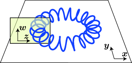
Figure 1: Snap shot of a toroidal spiral string. The string coils around a torus embedded in the four-dimensional Euclid space $(x,y,z,w)=(\rho\cos\phi,\rho\sin\phi,\zeta\cos\psi,\zeta\sin\psi)$.

Next, we consider the toroidal spiral strings in the five-dimensional Myers-Perry metric

$$ds^{2}= -dt^{2}+\frac{2M}{\Sigma}\Big{(}dt-a\sin^{2}\theta d\phi-b\cos^{2}\theta d\psi\Big{)}^{2}$$ (15)

$$+\frac{\Sigma dr^{2}}{\Delta}+\Sigma d\theta^{2}+(r^{2}+a^{2})\sin^{2}\theta d\phi^{2}$$ (16)

$$+(r^{2}+b^{2})\cos^{2}\theta d\psi^{2}\ ,$$ (17)

where

$$\Delta=\frac{(r^{2}+a^{2})(r^{2}+b^{2})}{r^{2}}-2M,$$ (18)

$$\Sigma=r^{2}+a^{2}\cos^{2}\theta+b^{2}\sin^{2}\theta,$$ (19)

and $a,b$, and $M$ are parameters related to two independent rotations and mass, respectively.

The metric of the orbit space for toroidal spiral strings, which is associated with the Killing vector (4), is

$$ds_{4}^{2}= (\xi\cdot\xi)h_{\mu\nu}dx^{\mu}dx^{\nu}$$ (20)

$$= -\Big{[}(\xi\cdot\xi)-\frac{2M}{\Sigma}\Big{(}(r^{2}+a^{2})\sin^{2}\theta+\alpha^{2}(r^{2}+b^{2})\cos^{2}\theta\Big{)}\Big{]}dt^{2}$$ (21)

$$+\frac{(\xi\cdot\xi)\Sigma}{\Delta}dr^{2}+(\xi\cdot\xi)\Sigma d\theta^{2}-\frac{2M\cos^{2}\theta\sin^{2}\theta}{\Sigma}\Big{[}b(r^{2}+a^{2})-\alpha a(r^{2}+b^{2})\Big{]}dtd\bar{\varphi}$$ (22)

$$+\frac{\cos^{2}\theta\sin^{2}\theta}{\Sigma}\Big{[}2M\Big{(}r^{2}(a^{2}\sin^{2}\theta+b^{2}\cos^{2}\theta)+a^{2}b^{2}\Big{)}+\Sigma(r^{2}+a^{2})(r^{2}+b^{2})\Big{]}d\bar{\varphi}^{2},$$ (23)

where $\bar{\varphi}=\psi-\alpha\phi$, and the norm of $\xi$ is given by

$$\xi\cdot\xi=(r^{2}+a^{2})\sin^{2}\theta+\alpha^{2}(r^{2}+b^{2})\cos^{2}\theta+\frac{2M}{\Sigma}(a\sin^{2}\theta+\alpha b\cos^{2}\theta)^{2}.$$ (24)

Since the metric (23) has the Killing vectors $\partial_{t}$ and $\partial_{\bar{\varphi}}$, the corresponding canonical momenta are constants of motion. Setting $p_{t}=-E=const.$ and $p_{\bar{\varphi}}=L=const.$, we get the reduced Hamiltonian as

$$H =\frac{N}{2}\left[(\xi\cdot\xi)^{-1}\left(h^{rr}p_{r}^{2}+h^{\theta\theta}p_{\theta}^{2}\right)+V_{\rm eff}(r,\theta)\right],$$ (25)

where $h^{rr}={\Delta}/{\Sigma}$ and $h^{\theta\theta}={1}/{\Sigma}$, and

$$V_{\rm eff}(r,\theta)= -\frac{1}{\Sigma}\left((r^{2}+2M)+\frac{4M^{2}}{\Delta}+(a^{2}\cos^{2}\theta+b^{2}\sin^{2}\theta)\right)\frac{E^{2}}{\xi\cdot\xi}$$ (26)

$$+\frac{1}{\Sigma}\left(\frac{(a^{2}-b^{2})\Big{(}r^{2}(1-\alpha^{2})+(a^{2}-\alpha^{2}b^{2})\Big{)}-2M(a-\alpha b)^{2}}{r^{2}\Delta}+\frac{1}{\cos^{2}\theta}+\frac{\alpha^{2}}{\sin^{2}\theta}\right)\frac{L^{2}}{\xi\cdot\xi}$$ (27)

$$+\frac{4M(-b(r^{2}+a^{2})+\alpha a(r^{2}+b^{2}))}{r^{2}\Delta\Sigma}\frac{EL}{\xi\cdot\xi}+1.$$ (28)

The dynamical system of the toroidal spiral strings in the Myers-Perry black hole is reduced to the two-dimensional particle system specified by the Hamiltonian (25) with (28). A typical potential shape is drawn as a contour plot in Fig.2. There exists a stationary solution $r=r_{0}=const.$ and $\theta=\theta_{0}=const.$ at the local minimum of $V_{\text{eff}}(r,\theta)$.

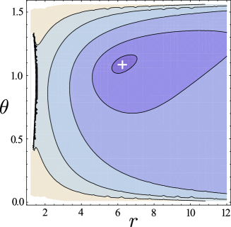
Figure 2: Contour plot of typical shape of the effective potential in the Myers-Perry metric. Parameters are chosen as $\alpha=2,L/E=3/2$, and black hole parameters are $2M=1,a=1/4,b=1/5$, for example. The local minimum of the potential exists at the mark ‘+’ in the figure.

To inspect conditions for existence of the stationary solution, we restrict ourselves to the non-rotational case $a=b=0$, for simplicity. By use of the variables $\rho:=r\sin\theta$ and $\zeta:=r\cos\theta$ which are used in Minkowski case, the effective potential (28) becomes

$$V_{\text{eff}}(\rho,\zeta) =\frac{E^{2}}{\rho^{2}+\alpha^{2}\zeta^{2}}\left(-1-\frac{2M}{\rho^{2}+\zeta^{2}-2M}\right)+\frac{L^{2}}{\rho^{2}+\alpha^{2}\zeta^{2}}\left(\frac{\alpha^{2}}{\rho^{2}}+\frac{1}{\zeta^{2}}\right)+1.$$ (29)

We can interpret the two terms in the first parenthesis as attractive terms by string tension and gravity, and two terms in the second parenthesis as centrifugal repulsion by $\phi$ and $\psi$ rotations, respectively.

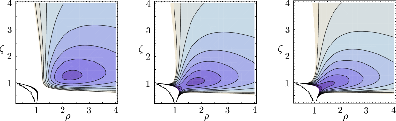
Figure 3: Contour plot of typical shapes of effective potential in the Schwarzschild-Tangherlini metric with $2M=1$. Parameters are chosen as $\alpha=2$, $L/E=0.7$(left), $L/E=0.62$(center), and $L/E=0.6$(right). Local minima of the effective potential appear in the left and center panels, while the local minimum disappears in the right panel.

The potential shapes are in Fig.3. As same as in the Minkowski case, we can find stationary solutions $\rho=\rho_{0}$ and $\zeta=\zeta_{0}$ at the minimum of $V_{\text{eff}}(\rho,\zeta)$. The explicit values of $\rho_{0}$ and $\zeta_{0}$ are given by solving the coupled algebraic equations

$$\partial_{\rho}V_{\rm eff}(\rho,\zeta)=0,\quad\partial_{\zeta}V_{\rm eff}(\rho,\zeta)=0,\quad\mbox{and}\quad V_{\rm eff}(\rho,\zeta)=0.$$ (30)

On a time slice $t=const.$, the stationary toroidal spiral string solution coils around a two-dimensional torus S${}^{1}\times$ S¹ of radii $\rho=\rho_{0}$ and $\zeta=\zeta_{0}$ that lies on S³ of the radius $r_{0}^{2}=\rho_{0}^{2}+\zeta_{0}^{2}$ which is surrounding the black hole.

In contrast to the flat case, because of the gravitational term, the minimum of $V_{\text{eff}}(\rho,\zeta)$ is a local minimum in the black hole case. The local minimum in the $\rho$-$\zeta$ plane moves with the value of $L/E$, and disappears if $L/E$ becomes less than a critical value for each $\alpha$.

We see from (30) that the local minimum points $(\rho_{0},\zeta_{0})$ for fixed $\alpha$ stay on the curve

$$(\rho_{0}^{2}+\zeta_{0}^{2})^{2}(\rho_{0}^{2}-\alpha^{2}\zeta_{0}^{2})+4M(1-\alpha^{2}){\rho_{0}^{2}\zeta_{0}^{2}}=0$$ (31)

in the $\rho$-$\zeta$ plane. In the case of $\alpha=1$, $\rho_{0}$ is simply equal to $\zeta_{0}$. The cross section of $V_{\text{eff}}(\rho,\zeta)$ in $\alpha=1$ case along the line $\zeta=\rho$ becomes

$$V_{\text{eff}}^{\alpha=1}\Big{|}_{\zeta=\rho}(\rho) =-\frac{E^{2}}{2\rho^{2}}\left(1+\frac{M}{\rho^{2}-M}\right)+\frac{L^{2}}{\rho^{4}}+1.$$ (32)

We easily find that the innermost radii are $\rho_{0}=\zeta_{0}=\sqrt{3M}$ (see Fig.4). For $\alpha\neq 1$ cases the curves (31) and innermost radii of stationary toroidal spirals are shown in Fig.5.

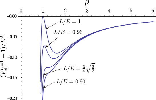
Figure 4: Cross sections of effective potential for $\alpha=1$ and various values of $L/E$ in the Schwarzschild-Tangherlini metric with $2M=1$. The local minimum disappears if $L/E=\frac{3}{4}\sqrt{\frac{3}{2}}$.

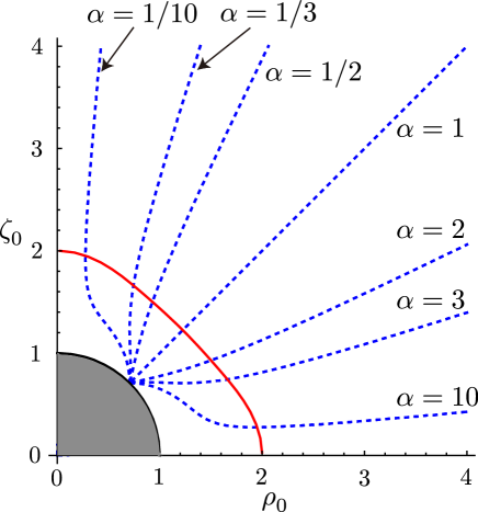
Figure 5: The radii $(\rho_{0},\zeta_{0})$ of innermost toroidal spiral strings are plotted (solid curve). The radii for stationary toroidal spirals stay on broken curves for fixed $\alpha$. Shaded region denotes inside the black hole horizon.

The behavior of the toroidal spiral strings around higher-dimensional black holes is analogous to the geodesic particles around four-dimensional black holes. The toroidal spiral strings would play a role of probes to reveal geometrical properties of higher-dimensional black holes. This similarity suggests that the toroidal spirals could be captured by a black hole and be settled into stationary states if they lose center of mass energy by any processes. Because strings in higher dimensions hardly intersect with othersJackson:2004zg , toroidal spirals could accumulate around a black hole like a cloud.

The toroidal spirals are characterized by commuting Killing vectors of which integral curves are closed in the target space. The stationary toroidal spirals are realized essentially by the balance of the string tension and the centrifugal force, it is straight forward to extend the solution in the case of black holes with more than five-dimensions. It is also possible to consider more complicated spiralling strings generated by more numbers of Killing vectors. Moreover, we can consider the black rings as play grounds of the toroidal spiral strings.

It is interesting problem to study the gravitational field around the toroidal spirals. Investigation of gravitational wave emission from the toroidal spirals would be important. In four-dimensions, it is well known that cusps commonly appear in the evolution of closed stringsKibble:1982cb . However, even if strings are closed in five-dimensions, as has been shown in this paper, they can be the stationary toroidal spirals without cusp. The difference comes from the dimensionality of the target space of the strings. It would be natural that the stationary toroidal spirals emit gravitational waves almost constantly in a long duration with periodic waveformsOgawa:2008yx in the higher-dimensional universe.

The toroidal spirals are extended sources of gravity which have two independent rotations. They would mimic gravitational fields of black rings in far regions. Toroidal spirals in six or more dimensions would supply hints to construct black ring solutionsEmparan:2007wm .

Though we mainly focus on the stationary solution of toroidal spirals in this article, investigation of the dynamics of toroidal spirals is a tractable issue. We will report integrability of the system in a separate paperIgata-Ishihara .

This work is supported by the Grant-in-Aid for Scientific Research No.19540305.

References

- (1) R. Emparan and H. S. Reall, ”Black Holes in Higher Dimensions”, Living Rev. Relativity 11, (2008), 6. URL (cited on 30 Oct. 2009): http://www.livingreviews.org/lrr-2008-6 .
- (2) R. C. Myers and M. J. Perry, Annals Phys. 172, 304 (1986).
- (3) V. P. Frolov and D. Stojkovic, Phys. Rev. D 67, 084004 (2003); Ibid. D 68, 064011 (2003) .
- (4) V. P. Frolov and D. Kubiznak, Phys. Rev. Lett. 98, 011101 (2007) .
- (5) V. P. Frolov and K. A. Stevens, Phys. Rev. D 70, 044035 (2004) .
- (6) D. Kubiznak and V. P. Frolov, JHEP 0802, 007 (2008) .
- (7) H. Ahmedov and A. N. Aliev, Phys. Rev. D 78, 064023 (2008) .
-
(8)
V. P. Frolov, V. Skarzhinsky, A. Zelnikov and O. Heinrich,
Phys. Lett. B 224, 255 (1989).
V. P. Frolov, S. Hendy and J. P. De Villiers, Class. Quant. Grav. 14, 1099 (1997). - (9) H. Ishihara and H. Kozaki, Phys. Rev. D 72, 061701 (2005).
-
(10)
C. J. Burden and L. J. Tassie,
Austral. J. Phys. 35, 223 (1982);
Ibid. 37, 1 (1984);
C. J. Burden, Phys. Rev. D 78, 128301 (2008). -
(11)
H. J. de Vega, A. L. Larsen and N. G. Sanchez,
Nucl. Phys. B 427, 643 (1994);
A. L. Larsen and N. G. Sanchez, Phys. Rev. D 50, 7493 (1994); Ibid. D 51, 6929 (1995);
H. J. de Vega and I. L. Egusquiza, Phys. Rev. D 54, 7513 (1996). -
(12)
K. Ogawa, H. Ishihara, H. Kozaki, H. Nakano and S. Saito,
Phys. Rev. D 78, 023525 (2008);
T. Koike, H. Kozaki and H. Ishihara, Phys. Rev. D 77, 125003 (2008);
H. Kozaki, T. Koike and H. Ishihara, arXiv:0907.2273 [gr-qc]. -
(13)
H. Ishihara and K. Matsuno, Prog. Theor. Phys. 116, 417 (2006);
K. Matsuno and H. Ishihara, arXiv:0909.0134 [hep-th]. - (14) M. G. Jackson, N. T. Jones and J. Polchinski, JHEP 0510, 013 (2005).
- (15) T. W. B. Kibble and N. Turok, Phys. Lett. B 116, 141 (1982).
- (16) K. Ogawa, H. Ishihara, H. Kozaki and H. Nakano, Phys. Rev. D 79, 063501 (2009).
- (17) R. Emparan, T. Harmark, V. Niarchos, N. A. Obers and M. J. Rodriguez, JHEP 0710, 110 (2007).
- (18) T.Igata and H.Ishihara, in preparation.