The long term X–ray spectral variability of AGN

Abstract

We present the results from the spectral analysis of more than 7,500 RXTE spectra of 10 AGN. Our main goal was to study their long term X–ray spectral variability. The sources in the sample are nearby, X-ray bright, and they have been observed by RXTE regularly over a long period of time ($\sim$7–11 years). High frequency breaks have been detected in their power spectra, and these characteristic frequencies imply time scales of the order of a few days or weeks. Consequently, the RXTE observations we have used most probably sample most of the flux and spectral variations that these objects exhibit. Thus, the RXTE data are ideal for our purpose. Fits to the individual spectra were performed in the 3–20 keV energy band. We modeled the data in a uniform way using simple phenomenological models (a power-law with the addition of Gaussian line and/or edge to model the iron K$\alpha$ emission/absorption features, if needed) to consistently parametrize the shape of the observed X–ray continuum of the sources in the sample. We found that the average spectral slope does not correlate with source luminosity or black hole mass, while it correlates positively with the average accretion rate. We have also determined the (positive) “spectral slope – flux” relation for each object, over a flux range larger than before. We found that this correlation is similar in all objects, except for NGC 5548 which displays limited spectral variations for its flux variability. We discuss this global “spectral slope – flux” trend in the light of current models for spectral variability. We consider (i) intrinsic variability, expected e.g. from Comptonization processes, (ii) variability caused by absorption of X-rays by a single absorber whose ionization parameter varies proportionally to the continuum flux variations, (iii) variability resulting from the superposition of a constant reflection component and an intrinsic power-law which is variable in flux but constant in shape, and, (iv) variability resulting from the superposition of a constant reflection component and an intrinsic power-law which is variable both in flux and shape. Our final conclusion is that scenario (iv) provides the best fit to the data of all objects, except for NGC 5548.

1 Introduction

The current paradigm for the central source in AGN postulates a black hole (BH) with a mass of $10^{6}-10^{9}$ M_⊙, and a geometrically thin, optically thick accretion disc that presumably extends to the innermost stable circular orbit around the black hole. This disc is supposed to be responsible for the broad, quasi-thermal emission component in the optical-UV spectrum of AGN (the so-called Big Blue Bump). At energies above $\sim$2 keV, a power-law like component is observed. This is attributed to emission by a hot corona ($T\sim 10^{8}-10^{9}$ K) overlying the thin disc. The corona up-Comptonizes the disc soft photons to produce the hard ($E\sim 2-100$ keV) X-ray emission. An Fe K$\alpha$ line is also detected, produced either by fluorescence on cold matter at $E=6.4$ keV or by photoionization of H-like or He-like Fe at 6.9 keV and 6.7 keV, respectively. This feature is believed to be emitted on the surface of the accretion disc, from the reprocessing of the X-rays. In many cases the line is resolved, and its width can, in theory, constrain the position of the inner radius of the disc and the spin of the central BH.

The AGN X–ray emission is strongly variable, even on time scales as short as a few hundred seconds, both in flux and in the shape of the observed energy spectrum. These variations can provide information on the physical conditions, the size, and the geometry of the X–ray emitting region. Regarding the flux variability, although the broad band power spectra of AGN are not well understood, the identification of characteristic time scales in them, combined with the large range in the masses of the BHs that have been studied so far, can constrain (to some degree) the size and the geometry of the X–ray source (e.g. M^cHardy et al., 2006). On the other hand, recent detailed studies of the spectral variations observed in a few objects provide valuable details of the physical conditions of the X–ray reprocessing (Miniutti et al., 2007, see e.g.) and/or on the physical properties of absorbing material which may exist close to the central source (see e.g. Miller, Turner & Reeves, 2008).

Progress in settling alternative interpretations of the observed spectral variability can be made by correlating the spectral and timing properties in AGN. Along this line, in a recent paper (Papadakis et al., 2009) we studied 11 nearby, X–ray bright Seyferts, which have been intensively observed over the last two decades by the Rossi X-ray Timing Explorer (RXTE). We detected a positive correlation between their mean spectral slope and the characteristic break frequency, $\nu_{\rm br}$, at which the power spectrum changes its slope from -1 to -2. To the extent that this frequency corresponds to a (still unknown) characteristic time scale of the X–ray source, this correlation suggests that the mean X–ray spectral slope in AGN is determined by a fundamental parameter of the system, most probably its accretion rate. If true, this result has important implications on current Comptonization models.

In this work we use the results from the model fitting of thousands of RXTE spectra of 10 AGN that were included in the sample of Papadakis et al. (2009). Our prime goal is to study in detail the X–ray spectral variability of each object. Although the spectral resolution of RXTE is not as good as that of Chandra, XMM-Newton or Suzaku, the RXTE data sets that we used are ideal for our purpose. First, the sources in the sample are nearby and X-ray bright. As a result, their X–ray spectral shape can be accurately determined even from relatively short ($\sim$1–2 ksec) RXTE observations. Second, each source in the sample was observed regularly (more than 200–300 times, and in a few cases more than a thousand times) over a long period of time (of the order of 7–11 years). This is contrary to typical Chandra and XMM-Newton observations of individual AGN, which usually span a period of a few days (maximum). Third, the characteristic frequencies of the objects imply time scales of the order of a few days or weeks. Consequently, the RXTE observations we have used most probably sample most of the flux and spectral variations that they exhibit.

A subsample of the observations we study have already been studied by Papadakis et al. (2002). These authors used hardness ratios in various energy bands to study the spectral variability of four objects, namely NGC 5548, NGC 5506, NGC 4051 and MCG -6-30-15. In the present work we studied many more observations of these objects and we have also analysed data for six more Seyferts. Furthermore, instead of computing hardness ratios, we fitted each spectrum with the same phenomenological model of a “power law plus a Gaussian line” to derive the observed photon index, $\Gamma_{\rm obs}$. In this way, we parametrized all available 3–20 keV RXTE spectra of the sources in a uniform way. We then used the resulting best model fitting values to: i) determine the mean spectral slope for each object and investigate its correlation with the main source parameters such as BH mass, accretion rate and luminosity, and ii) construct their long term “spectral slope vs. flux” relations. For the reasons explained above, we believe that we determined the flux related spectral variability in these sources more accurately than before.

Several possible reasons for the observed X–ray spectral variability in AGN have been proposed in the past. The simplest possibility is that the $\Gamma_{\rm obs}$ variations correspond to intrinsic variations in continuum slope (e.g. Haardt, Maraschi & Ghisellini, 1997; Coppi, 1999; Beloborodov, 1999). For example, Nandra & Papadakis (2001) have showed that the X-ray spectral changes in NGC 7469 are intrinsic and respond to the UV-soft photon input variations, exactly as one would expect in the case of thermal Comptonization models. However, there has also been certain observational evidence that the $\Gamma_{\rm obs}$ variations originate as a result of superposition of different spectral components with different variability properties. One such possibility is a spectrum composed of a constant reflection component and a variable, in normalization only, power-law like continuum of constant slope (e.g. Taylor, Uttley & M^cHardy, 2003; Ponti et al., 2006; Miniutti et al., 2007, and references therein). Another possibility is a constant slope power law which varies in flux and complex variations in an absorber, e.g. its ionization state and/or the covering factor of the source (see recent review by Turner & Miller, 2009).

One of our main result is that the X–ray spectral slope steepens with increasing flux in a similar way for all the objects in the sample. This similarity implies that, although all the above mentioned mechanisms may operate in AGN, it is just one of them which is mainly responsible for the observed spectral variability in AGN.

The paper is organized as follows. In Section 2, we discuss the data selection and reduction, and we also describe the phenomenological models that we used to parametrize the shape of AGN continuum. In Section 3, we report the spectral fitting results, and the results from the spectral variability study. In Section 4, we discuss our findings and compare them with predictions of several spectral variability models. We give our conclusions in Section 5.

2 Data Reduction and Analysis

Table 1: Summary of the RXTE observations and properties of the AGN in the sample. In column 2, $N$ is the total number of observations considered for a given AGN. Dates of the first and last observation are listed in column 3. The luminosity distances, $D$, and redshifts, $z$, listed in columns 4 and 5, were taken form the NED database. In column 6 we list black hole mass estimates.

Source	$N$	Start/End	Lum. Distance	Redshift	$M_{\rm BH}$
			D / Mpc	z	$\times 10^{6}$ M⊙
(1)	(2)	(3)	(4)	(5)	(6)
Fairall 9	671	1996-11-03/2003-03-01	199	0.047	255
Akn 564	505	1996-12-23/2003-03-04	98.6	0.025	1.9
Mrk 766	219	1997-03-05/2006-11-07	57.7	0.013	3.6
NGC 4051	1257	1996-04-23/2006-10-01	12.7	0.002	1.9
NGC 3227	1021	1996-11-19/2005-12-04	20.4	0.004	42.2
NGC 5548	866	1996-05-05/2006-11-06	74.5	0.017	67.1
NGC 3783	874	1996-01-31/2006-11-08	44.7	0.010	29.8
NGC 5506	627	1996-03-17/2004-08-08	29.1	0.006	28.8
MCG-6-30-15	1214	1996-03-17/2006-12-24	35.8	0.008	6.8
NGC 3516	250	1997-03-16/2006-10-13	37.5	0.009	42.7

Table 2: Quality of the various model fits to the data. The number of model-fit “successes”, $n_{s}$, and global propabilities, P_c (see Sec. 2.2 for details), are listed for various models.

	PL		PLG		ePLGa		ePLGb		ePLGc
Source	$n_{s}$	Pc	$n_{s}$	Pc	$n_{s}$	Pc	$n_{s}$	Pc	$n_{s}$	Pc
(1)	(2)	(3)	(4)	(5)	(6)	(7)	(8)	(9)	(10)	(11)
Fairall 9	642	0.81
Akn 564	486	0.92
Mrk 766	208	0.54
NGC 4051	1167	$5\times 10^{-4}$	1199	0.75
NGC 3227	919	$<10^{-5}$	980	0.94
NGC 5548	802	$1\times 10^{-3}$	827	0.77
NGC 3783	635	$<10^{-5}$	799	$<10^{-5}$	821	0.09
NGC 5506	382	$<10^{-5}$	556d	$<10^{-5,d}$	586d	0.05d
MCG-6-30-15	925	$<10^{-5}$	1076	$<10^{-5}$	1136	0.02	1147	0.22
NGC 3516	160	$<10^{-5}$	221	$<10^{-5}$	227	0.004	227	0.004	231	0.05

^a the edge energy fixed at 7.1 keV

^b the edge energy allowed to vary

^c both the line and edge energies allowed to vary

^d PLG or ePLG model plus cold absorption with $N_{\rm H}=3.7\times 10^{22}$ cm^-2

2.1 Data selection and reduction

In Tab. 1, we list the 10 AGN in our sample, some of their properties (distance, redshift and BH mass estimates), and details of the RXTE observations we used in this work. We used the Peterson et al. (2004) estimates, from reverbaration mapping, for the BH mass (M${}_{\rm BH})$ in Fairall 9, NGC 4051, NGC 3227, NGC 5548, NGC 3783, and NGC 3516. In the case of Mrk 766 and MCG-6-30-15 we used the stellar velocity dispecrsion measurements of Botte et al. (2004) and M^cHardy et al. (2005), respectively, and the Tremaine et al. (2002) $M_{\rm BH}-\sigma$ relation to estimate BH mass. The BH mass estimates for Ark 564 and NGC 5506 were taken from Zhang & Wang (2006) and Wang & Zhang (2007), respectively. They were also based on the Tremaine et al. (2002) M${}_{\rm BH}-\sigma$ relation, although in this case the stellar velocity dispecrsion was obtained from the FWHM of the O_III line, using the FWHM O${}_{\rm III}-\sigma$ relation of Greene & Ho (2005). Since the reverbaration mapping estimates have been obtained by “forcing” the AGN $M_{\rm BH}-\sigma$ relationship to have the same normalization as the $M_{\rm BH}-\sigma$ relationship for quiescent galaxies (Peterson et al., 2004), we belive that the usege of two different M_BH determination methods should not add significant scatter to the correlations we present below.

For each object we considered all the RXTE observations that were performed until the end of 2006. Some of these objects were monitored with RXTE for as long as 10 years. The reason we chose to study these AGN is precisely because they have been observed frequently by RXTE. They are all nearby, X–ray bright, Type I objects (except for NGC 5506, which is optically classified as Type II Seyfert). Their central BH mass ranges from $\sim$2$\times 10^{6}$ M_⊙ to $\sim$2$\times 10^{8}$ M_⊙, and their accretion rate from a few percent of the Eddington limit (in NGC 3227) to almost close to this limit (in Ark 564; see e.g. M^cHardy et al. 2006). Consequently, they could be considered as representative of the Seyfert population in the local Universe.

We used data from the Proportional Counter Array (PCA; Jahoda et al., 1996). The typical duration of each observation was $\sim$1–2 ksec. The data were reduced using FTOOLS v.6.3. The PCA data were screened according to the following criteria: the satellite was out of the South Atlantic Anomaly (SAA) for at least 30 min, the Earth elevation angle was $\geq 10^{\circ}$, the offset from the nominal optical position was $\leq 0^{\circ}\!\!.02$, and the parameter ELECTRON-2 was $\leq 0.1$.

We extracted STANDARD-2 mode, 3–20 keV, Layer 1, energy spectra from PCU2 only. For background subtraction we used the appropriate background model for the faint objects available from RXTE data analysis web-pages. The background subtracted spectra were rebinned using grppha so that each bin contained more than 15 photons for the $\chi^{2}$ statistic to be valid. We considered only these data sets for which binning resulted in at least 15 PHA channels. We used PCA response matrices and effective area curves created specifically for the individual observations by pcarsp.

2.2 Modeling the spectral shape of the AGN

Fits to the individual spectra were performed in the energy range 3–20 keV, where the PCA is most sensitive, using the XSPEC v.11.3.2 software package (Arnaud, 1996). Our prime aim was to parametrize in a uniform way (i.e. by fiting the same model to all the observations) the shape of the observed X–ray continuum of the sources in our sample. We first fitted a simple power-law model (hereafter PL) to all the individual spectra of all sources. In the cases when the global goodness of the PL fit was unacceptable, we added additional spectral components. The form of these components was chosen based on visual examination of the PL fit residuals in the cases when the model did not fit the data well.

We did not consider the Galactic absorption effects as the Galactic column to all sources is so low that cannot affect the spectrum above 3 keV. In the case of NGC 5506, all models were modified by cold absorption using wabs in XSPEC, with the hydrogen column density fixed at N${}_{\rm H}=3.7\times 10^{22}$ cm^-2 (Perola et al., 2002).

We assumed that a model fits well the spectrum of an individual observation if the probability of accepting the null hypothesis, $p_{\rm null}$, is larger than 0.05. Given that the number of observations for each AGN is quite large, it is possible that $p_{\rm null}<0.05$ in some cases, even if the model is the correct one. Therefore, the global goodness of a model fit to all the spectra of each source had to be judged in a statistical way. One method to achieve this is to consider the fit to the individual spectra as a “success” when $p_{\rm null}>0.05$, and as a “failure” otherwise. Under the hypothesis that the model is the correct one, the probability of a “success” (“failure”) is $p_{\rm s}=0.95$ (1-$p_{\rm s}$ = 0.05), by definition. In this approach, the model fit to each spectrum can be considered as a Bernoulli trial.

For a given source and a given model we recorded the total number of spectra, $N$, the number of model-fit “successes”, $n_{\rm s}$, and the number of model-fit “failures”, $n_{\rm f}$. Then, we used the binomial distribution to estimate the probability, P_c, that the number of “failures” will be larger than $n_{\rm f}$ in $N$ trials by chance. This is equal to the probability that the numbers of “successes” will be smaller than $n_{\rm s}$. Therefore, P_c can be estimated as

$$P_{\rm c}=\sum_{j=0}^{n_{\rm s}}{N\choose j}p_{\rm s}^{j}(1-p_{\rm s})^{N-j}.$$ (1)

We accepted that a model fits globally the spectra of a source if $0.05<P_{\rm c}<0.95$. We report below the results from the various model fits to the data of all sources.

2.2.1 “Power-law” model fits

The PL model fited well the spectra of only three sources: Fairall 9, Akn 564 and Mkn 766 ($n_{\rm s}$ and P_c values are listed in the second and third columns of Tab. 2). In the remaining 7 objects we clearly detected 6–7 keV residua indicative of an iron K_α line (see Fig. 1).

2.2.2 “Power-law plus line” model fits

Motivated by shape of the PL best model fit residua around 6–7 keV, we added a Gaussian component to account for the K$\alpha$ iron line in these spectra (powerlaw+gaussian in XSPEC, hereafter PLG). In all cases, the iron line energy and width were fixed at 6.4 keV and 0.1 keV, respectively. The goodness of the new model fits improved and became acceptable in NGC 4051, NGC 3227 and NGC 5548 ($n_{\rm s}$ and P_c values for the PLG model are listed in columns 4 and 5 of Tab. 2).

2.2.3 “Power-law plus line plus edge” model fits

Figure 2 shows the best PLG model fit residua in the case of an unacceptable model fit to a spectrum of (a) NGC 5506, (b) NGC 3783, (c) MCG -6-30-15, and (d–e) NGC 3516. The best-fit model residuals indicate the presence of an edge-like feature around $\sim$7 keV. We therefore considered a edge*(powerlaw+gauss) model in XSPEC (ePLG hereafter). We kept the edge energy fixed at 7.1 keV (the threshold energy for neutral iron) and we re-fitted the individual spectra of these sources.

The global fit became acceptable in the case of NGC 5506 and NGC 3783. The optical depth of the edge, $\tau$, was detected at the 2$\sigma$ significance level in 298 out of 627 observations, in the case of NGC 5506, and in 319 out of 874 observations in NGC 3783. The respective $n_{\rm s}$ and P_c values listed in columns 6 and 7 of Tab. 2.

In MCG-6-30-15 the model fit improved significantly, and the model became acceptable, when we allowed the energy of the edge to vary between 6 and 10 keV (results are listed in columns 8 and 9 of Tab. 2). The edge was detected at the 2$\sigma$ significance level in 863 out of 1214 data sets. Using the best fit results for these spectra only, we estimated that $\overline{E}_{\rm edge}\sim 7.4$ keV, an energy that is indicative of absorption by ionized iron. However, the standard deviation of the best fit edge energy values is substantial ($\sigma\sim 1$ keV), which suggests that one should treat this result with caution (see discussion in Section 2.2.5).

In the case of NGC 3516 we did not record an improvement to the global fit of the ePLG model, even when the edge energy was allowed to vary (compare columns 6 and 7, and 8 and 9 of Tab. 2). Thus, we thawed the energy of the iron line and allowed it to vary between 5.5 and 7.5 keV. This extra modification provided a statistically acceptable global fit (the $n_{\rm s}$ and P_c values listed in columns 10 and 11 in Tab. 2 correspond to this model). The average line energy, and its standard deviation, calculated for the data sets where the line is detected at the 2$\sigma$ significance level (117 of 250) were $6.1$ and 0.3 keV, respectively. The absorption edge was detected at the 2$\sigma$ significance level in 122 out of the 250 spectra of this source. Using the best fit results of these observations only, we calculated that the average energy of the absorption edge, and its standard deviation, were $\overline{E}_{\rm edge}=7.9$ and $\sigma=1.1$ keV, respectively.

2.2.4 Summary of the acceptable model fits

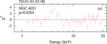
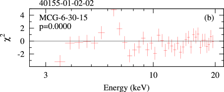
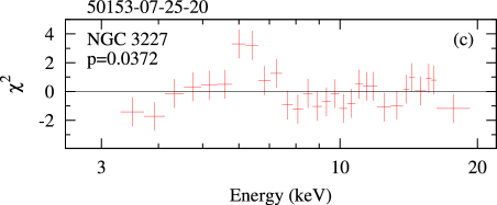
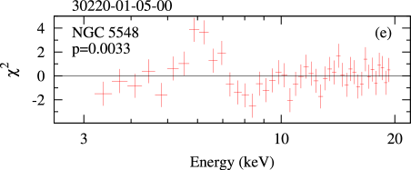
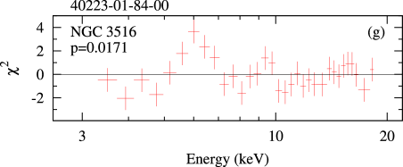
Figure 1: Contribution to $\chi^{2}$ for the PL model fits to the data of (a) NGC 4051 (obsid 70141-01-01-00), (b) MCG-6-30-15 (40155-01-02-02), (c) NGC 3227 (50153-07-25-20), (d) NGC3783 (40152-04-65-00), (e) NGC 5548 (30220-01-05-00), (f) NGC 5506 (50153-05-67-10), and (g) NGC 3516 (40223-01-84-00). The fit probabilities are indicated on each panel. Residuals indicative of an iron K$\alpha$ line are visible in the 5–7 keV band.

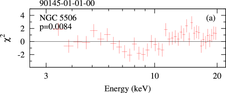
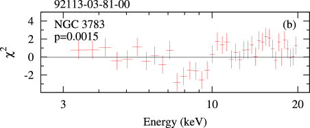
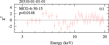
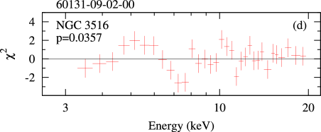
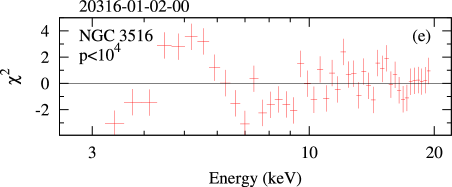
Figure 2: Contributions to $\chi^{2}$ for the PLG best fit models applied to exemplary data of (a) NGC 5506 (obsid 90145-01-01-00), (b) NGC 3783 (obsid 92113-03-81-00), (c) MCG-6-30-15 (obsid 20310-01-01-01) and (d–e) NGC 3516 (obsids 60131-09-02-00 and 20316-01-02-00). The fit probabilities are indicated on each panel.

Figure 3: The average $\Gamma_{\rm obs}$ (a) and EW of the iron line (b) in NGC 3516 for different spectral models. The model labels are M1 – PL; M2 – PLG; M3 – ePLG; M4 – same as M3 but with variable edge energy, $E_{\rm edge}$; M5 – same as M3 but with variable line energy, $E_{\rm line}$; M6 – same as M3 but with variable both $E_{\rm edge}$ and $E_{\rm line}$. The error-bars represent standard errors on the mean. The horizontal lines indicate the average $\overline{\Gamma_{\rm obs}}$ and $\overline{EW}$.

• A simple PL model describes well the spectra of Fairall 9, Akn 564 and Mkn 766.

• In NGC 4051, NGC 3227, and NGC 5548 a statistically acceptable global fit to the data is obtained with the PLG model.

• In NGC 3783 and NGC 5506, the addition of an absorption edge with energy fixed at 7.1 keV is needed to achieve an acceptable model fit (ePLG).

• In MCG 6-30-15 the best global fit is reached by the ePLG model but only when the edge energy is allowed to vary (the resulting mean edge energy is $\overline{E}_{\rm edge}\sim 7.4$ keV).

• Finally, the same ePLG model provides an acceptable global fit to the NGC 3516 spectra but only when both the energy of the iron line and the energy of the absorption edge were left free to vary ($\overline{E}_{\rm line}\sim 6.1$, and $\overline{E}_{\rm edge}\sim 7.95$).

In Section 3, we report the results from: (a) the study of the correlation of the average spectral slope with other source parameters, such as luminosity, accretion rate and black hole mass, (b) the study of the spectral slope variations as a function of the source luminosity for each object in the sample, and (c) the study of the average line’s equivalent width variations with other source parameters. In each case, we use the appropriate, for each source, best fitting slope, $\Gamma_{\rm obs}$, and line’s EW values.

We do not consider the implications from the “variable edge energy” model fits to MCG -6-30-15 or from the “variable iron line and edge energy” model fits to NGC 3516. We believe that the $E_{\rm edge}$ and $E_{\rm line}$ best fit values from these model fits should be treated with caution due to the low energy resolution of the PCA instrument. The residua plot in Figs. 2d–e show this clearly in the case of NGC 3516. It is the line-like positive residual at $\sim$5 keV that forces the best fit iron line energy to be less than 6.4 keV in this case. However, we can also get a good fit to the the spectrum from e.g. the 20316-01-02-00 observation of NGC 3516 (Fig. 2e) if we consider the ePLG model with $E_{\rm line}$ and $E_{\rm edge}$ kept fixed at 6.4 keV and 7.1 keV, respectively, together with intrinsic neutral absorption, i.e. if we add a wabs component to the model and we let N_H to be a free model parameter.

We note that in the case of NGC 5506, NGC 3783, MCG 6-30-15 and NGC 3516, the $\Gamma_{\rm obs}$ values were not dramatically affected when we added an absorption edge or when we let $E_{\rm edge}$ or $E_{\rm line}$ to vary freely during the model fitting process. For example, Fig. 3a shows the mean $\Gamma_{\rm obs}$ for NGC 3516 in the case of all 6 models that we applied to its individual spectra (PL, PLG, ePLG and its modifications: ePLG model with variable $E_{\rm edge}$ and/or $E_{\rm line}$). Despite the fact that, statistically speaking, models 1–5 are not formally acceptable, the mean best fit spectral slope values are almost identical. The largest difference is the one between $\overline{\Gamma}_{\rm obs}$ in the case of the PL model (M1 in Fig. 3) and in the case of the ePLG model when both the edge and line energies are left free to vary (M6 in Fig. 3). Although the difference between the mean $\Gamma$’s is statistically significant (the error-bars show standard errors on $\overline{\Gamma}$), it is so small ($\sim 0.1$) that it cannot affect any of the results we discuss in Section 3.

We reached the same conclusion for the mean EW of the iron line. In Fig. 3b, we plot $\overline{\rm EW}$ in the case of the 5 models that include an emission line component. The averages were calculated over the data-sets in which the line was detected at 2$\sigma$ level. All five measurements are in agreement with each other (again, the error-bars show standard errors on $\overline{\rm EW}$). The largest difference is the one between the average EW in the case of model M4 and model M6 ($\sim$100 eV). Taking into account their errors, the two measurements are consistent with each other, and so this difference does not affect any of the conclusions we present in Section 3.

3 Spectral variability analysis

Table 3: Variability properties of $\Gamma_{\rm obs}$ and $L_{\rm 2-10}$ based on the best-fit model parameter values.

Target	$\overline{\Gamma}_{\rm obs}$	$\chi^{2}/d.o.f.$	$F_{\rm var}$	$\overline{L}_{\rm 2-10}$	$\chi^{2}/d.o.f$	$F_{\rm var}$
			(%)	($\times 10^{42}$) erg s-1		(%)
Fairall 9	1.794$\pm$0.006	1.3	3.7$\pm$0.3	102$\pm$1	16	26.0$\pm$0.4
Ark 564	2.48 $\pm$0.01	1.6	5.0$\pm$0.3	25.5$\pm$0.4	20	30.7$\pm$0.3
Mrk 766	2.02 $\pm$0.01	2.3	4.6$\pm$0.4	10.6$\pm$0.2	55	30.3$\pm$0.5
NGC 4051	1.842$\pm$0.009	6.9	14.9$\pm$0.3	0.493$\pm$0.007	83	49.7$\pm$0.2
NGC 3227	1.552$\pm$0.008	7.1	13.7$\pm$0.2	1.86$\pm$0.03	109	48.0$\pm$0.2
NGC 5548	1.735$\pm$0.004	2.1	2.9$\pm$0.2	28.8$\pm$0.4	196	39.4$\pm$0.2
NGC 3783	1.616$\pm$0.004	2.5	4.7$\pm$0.1	17.0$\pm$0.1	111	23.2$\pm$0.1
NGC 5506	1.800$\pm$0.003	2.4	3.1$\pm$0.1	10.2$\pm$0.1	169	22.79$\pm$0.09
MCG-6-30-15	1.731$\pm$0.005	3.6	7.2$\pm$0.2	7.48$\pm$0.06	93	27.2$\pm$0.1
NGC 3516	1.40 $\pm$0.01	7.6	14.2$\pm$0.5	6.5$\pm$0.2	179	41.3$\pm$0.3

Figure 4: The RXTE light curves of $\Gamma_{\rm obs}$ and $L_{\rm 2-10}$ for objects with the best (NGC 4051 and MCG-6-30-15, a–b) and worst (NGC 3516 and Mrk 766, c–d) time coverage.

Figure 5: Relations between the average photon index, $\overline{\Gamma}_{\rm obs}$, and (a) BH mass, (b) average 2–10 keV luminosity, and (c) average mass accretion rate in Eddington units. The correlation in (c) is best described with a power-law, $\overline{\Gamma}_{\rm obs}\propto\overline{\dot{m}}_{\rm X,E}^{~{}0.08\pm 0.02}$ (solid curve).

Figure 6: Relations between the average EW of the iron line and the average (a) 2–10 luminosity, (b) mass accretion rate, and (c) photon index. The solid line in panel (a) indicates the best fit relation $\overline{\rm EW}\propto\overline{L}_{\rm 2-10}^{~{}-0.23\pm 0.06}$.

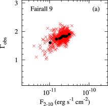
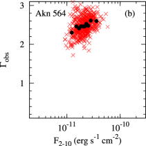
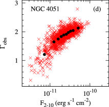
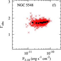
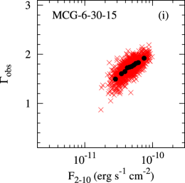
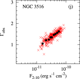
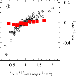
Figure 7: Dependence of $\Gamma_{\rm obs}$ on $F_{\rm 2-10}$ for all AGN in the sample. (a–j) The individual data (crosses) are shown together with the binned data (filled circles, see Sec. 3.3 for details of binning). Errors on the binned data are plotted but are smaller than the size of the symbols. (k) Binned data of NGC 3516 resulting from the simple power-law model (filled circles) and power-law model modyfied by a Gaussian line and absorption edge with variable line and edge energies(open circles; models M1 and M6 in Fig. 4, see Sec. 3.3 for details). (l) Binned $\Gamma-F_{\rm 2-10}$ data of all AGN. Fluxes are normalized to the respective $\overline{F}_{\rm 2-10}$, and we have subtracted the respective $\overline{\Gamma}_{\rm obs}$ from the spectral slope values. NGC 5548 (filled squares) follows a different “slope vs. flux” relation than the other AGN (open circles).

Figure 4 shows $\Gamma_{\rm obs}$ and the X-ray luminosity, $L_{\rm 2-10}$ plotted as a function of time for NGC 4051, MCG-6-30-15, NGC 3516 and Mrk 766. The first two objects are representative of sources observed by RXTE frequently (on average every $2-3$ days), between 1996 and 2006. On the other hand, NGC 3516 and Mkn 766 were systematically observed by RXTE only between the years 1999–2002 and 2004–2007, respectively. Outside of these dates data for these sources are scarce. Their light curves are representative of sources which were observed less than $\sim$700 times by RXTE from the start of the mission until the end of 2006.

The (unweighted) mean photon indices, $\overline{\Gamma}_{\rm obs}$, and 2–10 keV luminosities, $\overline{L}_{\rm 2-10}$, for the sources in our sample are listed in Tab. 3 (the standard error on $\overline{\Gamma}_{\rm obs}$ and $\overline{L}_{\rm 2-10}$ are very small, mainly because of the large number of data points). Application of the standard $\chi^{2}$ test to the $\Gamma_{\rm obs}$ and $L_{\rm 2-10}$ light curves suggests that all sources show significant spectral and flux variations (reduced $\chi^{2}$ values are listed in Tab. 3; the number of data points is large enough that even in the case when $\chi^{2}/d.o.f.\sim 1.3$–1.4 the variations we detected are significant at more than the 3$\sigma$ level).

To further quantify the variability properties of the AGN in our sample, we calculated the excess variance, $\sigma^{2}_{\rm xs}$, of the $\Gamma_{\rm obs}$ and $L_{\rm 2-10}$ light curves as follows,

$$\sigma^{2}_{\rm xs}=\frac{1}{n_{s}}\sum_{i=1}^{n_{s}}(x_{i}-\overline{x})^{2}-\frac{1}{n_{s}}\sum_{i=1}^{n_{s}}\sigma^{2}_{{\rm err,}i}.$$ (2)

The excess variance is a measure of the scatter about the mean in a light curve, corrected for the contribution expected from the experimental errors. In the formula above, $x$ stands either for $\Gamma_{\rm obs}$ or $L_{\rm 2-10}$, and $\sigma^{2}_{err,i}$ is the arithmetic mean of the upper and lower 90% confidence error on $\Gamma_{\rm obs}$ and $L_{\rm 2-10}$. We then estimated the fractional root mean square variability amplitude, $F_{\rm var}=\sqrt{\sigma^{2}_{\rm xs}/\overline{x}^{2}}$ and its error using equation (B2) in Vaughan et al. (2003) (this error accounts only for the uncertainty due to the experimental error in each point).

The results are listed in Tab. 3. In terms of variability amplitude, the flux variations are stronger (i.e. of larger amplitude) than the spectral variations. Furthermore, there seems to be a tendency for the objects with stronger flux variations to show stronger spectral variations as well. To quantify this correlation, we used the Kendall’s $\tau$ test. We found that $\tau=0.51$, which implies that the positive correlation between $F_{\rm var,\overline{\Gamma}}$ and $F_{\rm var,\overline{L}(2-10)}$ is significant at the 4% level.

3.1 Correlation between the average spectral slope and other source parameters

Figure 5 shows the average observed photon index, $\overline{\Gamma}_{\rm obs}$, plotted as a function of (a) BH mass, (b) average 2–10 luminosity, and (c) average X–ray mass accretion rate in Eddington units, $\overline{\dot{m}}_{\rm X,E}=L_{\rm 2-10}/L_{\rm E}$, where $L_{\rm E}=1.3\times 10^{38}$ M/M_⊙ ergs s^-1 is the Eddington luminosity of an AGN with a black hole mass M. This quantity should be representative of the total accretion rate (i.e. $L_{\rm bol}/L_{\rm E}$) of each source. For simplicity we will refere to it as the accretion rate hereafter. The errors on $\overline{\Gamma}_{\rm obs}$ plotted in Fig. 5 are the standard deviation of $\Gamma_{\rm obs}$ and we use them, instead of the standard error of the mean, to account for the scatter of the individual $\Gamma_{\rm obs}$ values about $\overline{\Gamma}_{\rm obs}$.

The solid lines plotted in Figs. 5a and 5b indicate the average spectral slope of all AGN in our sample. Individual points appear to scatter randomly about this line. These plots suggest that the average spectral shape does not correlate with either the average luminosity ($\tau=0.2$, $P_{\rm null}=0.42$) or BH mass ($\tau=-0.38$, $P_{\rm null}=0.13$). On the other hand, panel (c) in Fig. 5 implies a positive correlation between $\overline{\Gamma}_{\rm obs}$ and $\overline{\dot{m}}_{\rm X,E}$ ($\tau=0.51$, $P_{\rm null}=0.04$). Sources with a higher accretion rate appear to have steeper average spectra as well. We found that a power-law model of the form $y=\alpha x^{\beta}$ can fit well the data plotted in Fig. 5c ($\chi^{2}=8.14/8~{}d.o.f.$, $p_{\rm null}=0.42$). The best fitting parameters are: $\alpha=2.7\pm 0.3$, and $\beta=0.08\pm 0.02$ (the error on the slope indicates that the correlation between $\overline{\Gamma}_{\rm obs}$ and $\overline{\dot{m}}_{\rm X,E}$ is significant at the $4\sigma$ level).

3.2 Variations of the EW of the iron line

An iron $K_{\alpha}$ line is detected in many spectra of all sources (except for Akn 564, Fairall 9 and Mrk 766). To investigate the line’s EW variations, we considered the spectral fit results in the case when the line is detected at the 2$\sigma$ level in a spectrum of a source. The number of spectra which do show such a strong line, and the average equivalent width, $\overline{\rm EW}$, using the individual EW values from these spectra only, are listed in Tab. 4. The fourth column in Tab. 4 lists the $\chi^{2}$ values when we fit a constant to the EW light curves. The result is that we do not detect significant EW variations, except for NGC 5548, MCG -6-30-15, and NGC 3516. This is mainly due to the fact that, although the line is detected, the small exposure time of the individual RXTE observations did not allow the determination of the line’s EW with a high accuracy. We will present a more detailed study of the variability of the EW of the iron line in a forthcomming paper.

Panels (a), (b) and (c) in Fig. 6 show $\overline{\rm EW}$ plotted as a function of $\overline{L}_{\rm 2-10}$, $\overline{\dot{m}}_{\rm X,E}$, and $\overline{\Gamma}_{\rm obs}$. Fig. 6b and Fig. 6c imply that $\overline{\rm EW}$ does not correlate strongly with either accretion rate ($\tau=-0.05$, $P_{\rm null}=0.88$) or $\overline{\Gamma}_{\rm obs}$ ($\tau=-0.14$, $P_{\rm null}=0.65$). On the other hand, Fig. 6a suggests that the line’s EW anti-correlates with the source’s luminosity: the strength of the line decreases with increasing X-ray luminosity ($\tau=-0.52$, $P_{\rm null}=0.09$). This result is not statistically significant, most probably due to the small number of objects in the sample. However, this “equivalent width – luminosity” anti-correlation that we observe (the so-called Iwasawa-Taniguchi effect, Iwasawa & Taniguchi, 1993) is well established for nearby AGN (see e.g. Bianchi et al., 2007, and references therein). The solid line in Fig. 6a indicates the best power-law fit to the data. The best-fit slope of $-0.23\pm 0.06$ is consistent with the slope of $-0.17\pm 0.03$ found by Bianchi et al. (2007).

Table 4: The mean EW of the iron line and its standard deviation. N_2σ is the number of spectra with a $2\sigma$ detection of an iron line.

Target	N2σ	$\overline{\rm EW}$	$\chi^{2}$	$F_{\rm var}$
		(eV)		(%)
Fairall 9	-	-	-	-
Ark 564	-	-	-	-
Mrk 766	-	-	-	-
NGC 4051	13	682$\pm$351	41	-
NGC 3227	45	460$\pm$182	141	-
NGC 5548	19	248$\pm$184	101	37$\pm$14
NGC 3783	103	329$\pm$72	52	-
NGC 5506	177	242$\pm$63	88	-
MCG-6-30-15	47	498$\pm$335	260	38$\pm$8
NGC 3516	39	502$\pm$258	129	25$\pm$7

3.3 The spectral variability of each source

Figure 8: The binned “spectral slope - flux” data, as in Fig. 7, plotted with the best-fit function to the data plotted in Fig. 5c. The sources were split arbitrarly between panels (a) and (b) for clarity of presentation.

Crosses in panels (a–j) of Fig. 7 indicate the individual $(\Gamma_{\rm obs},F_{\rm 2-10})$ points for each AGN in the sample. To better illustrate the long-term, “observed spectral slope – flux” relation in these objects, we grouped the $(\Gamma_{\rm obs},F_{\rm 2-10})$ data in flux bins and calculated the (unweighted) mean flux and photon index in each bin. Each bin contains at least 20 measurements, and the number of bins is roughly equal for all sources. Filled circles in Fig. 7 indicate the (average spectral slope, average $F_{\rm 2-10}$) points. Both the binned and un-binned data points in Fig. 7 suggest that, in almost all objects, the spectrum softens with increasing 2–10 keV flux.

In Fig. 7k we plot the binned “spectral slope – flux” data for NGC 3516 using the best fit results of model M6 (filled circles) together with those when we used the best fit results of model M1 (open circles; this is the model that shows the largest discrepancy in $\overline{\Gamma}_{\rm obs}$ with the statistically acceptable model M6 for this source). We fitted a power-law model to the M1 and M6 data plotted in this panel, and the best fit slopes differ by 0.08$\pm 0.02$, with the M1 slope being flatter. Therefore, the exact shape of the “$\Gamma-F_{\rm 2-10}$” plots in Fig. 7 does depend on the choice of the model used to fit the individual spectra of the sources. However, the overall trend stays the same in both cases: the spectrum steepens with increasing flux.

In fact, the spectrum steepens with increasing flux in almost the same way in all sources. The opened circles in Fig. 7l indicate the binned “$\Gamma_{\rm obs}-F_{\rm 2-10}$” data for all sources. We did not use different symbols for each source in order to emphasize the fact that, in all sources, the spectral shape varies with flux in a similar way. The only exception is NGC 5548. Filled squares in Fig. 7l indicate the “$\Gamma_{\rm obs}-F_{\rm 2-10}$” data for this source. The spectral slope appears to stay roughly constant although the 2–10 keV flux varies by almost an order of magnitude. A positive correlation between spectral slope and X-ray flux may exist at the highest luminosity bins, but there is also a hint of an anti-correlation at the lowest luminosity bins.

The positive correlation between $\Gamma_{\rm obs}$ and $F_{\rm 2-10}$ can be translated into a correlation between $\Gamma_{\rm obs}$ and $\dot{m}_{\rm X,E}$, similarly to that between their average spectral slope and average accretion rate (compare Fig. 5c), but not necessarily the same. Figure 8 shows the binned $(\Gamma_{\rm obs},\dot{m}_{\rm X,E})$ data for all sources plotted together with the best-fit power-law model to the $(\overline{\Gamma}_{\rm obs},\overline{\dot{m}}_{\rm X,E})$ data from Fig. 5c. It is clear that, in at least some cases, such power-law cannot fit well the individual “observed spectral slope – accretion rate” relations.

To quantify the comparison between the average and the individual “observed spectral slope - accretion rate” relations, we fitted the ($\Gamma_{\rm obs},\dot{m}_{\rm X,E})$ data plotted in Fig. 8 with the same power-law model we used to fit the data shown in Fig. 5c. The model fits well the data of Akn 564 ($\beta_{\rm Akn564}=0.10\pm 0.01,\chi^{2}=15/8~{}d.o.f.$, $p_{\rm null}=0.06$), NGC 5506 ($\beta_{\rm NGC5506}=0.12\pm 0.01,\chi^{2}=8.1/8~{}d.o.f.$, $p_{\rm null}=0.43$), Mrk 766 ($\beta_{\rm Mrk766}=0.16\pm 0.01,\chi^{2}=6/8~{}d.o.f.$, $p_{\rm null}=0.75$), and NGC 3516 ($\beta_{\rm NGC3516}=0.32\pm 0.02,\chi^{2}=5.8/7~{}d.o.f.$, $p_{\rm null}=0.56$). Interestingly, $\beta_{\rm Akn564}$ and $\beta_{\rm NGC5506}$ are similar to the best fit slope in the case of the ($\overline{\Gamma}_{\rm obs},\overline{\dot{m}}_{\rm X,E})$ plot.

4 Discussion

The main aim of this work was to determine the shape of the X–ray continuum, and study its variability, in 10 X–ray luminous AGN which have been observed regularly with RXTE since 1996. We used a large number of spectra, which were taken regularly over a period of many years. As we argued in the introduction, since this time period is much larger than the characteristic time scale in these objects, it is possible that we have sampled the full range of their spectral variations. We therefore believe that we have determined, as accurately as it is possible at present, the “observed spectral slope – flux” relation for the AGN in the sample. In Section 4.1 we discuss the implications from the average “observed spectral slope - accretion rate” correlation reported in Section 3.1.

In Section 2.2.5 we argued that despite the limited spectral resolution of the PCA on board RXTE, the $\Gamma_{\rm obs}$ values we derived from the model fitting of the individual spectra of each source are representative of their actual X–ray spectral shape. However, this conclusion does not necessarily imply that $\Gamma_{\rm obs}=\Gamma_{\rm intr}$ ($\Gamma_{\rm intr}$ being the intrinsic slope of the X–ray continuum). Due to the short exposure of the individual RXTE observations and the limited resolution of the PCA on board RXTE, we cannot constrain the properties of any warm absorbing material that may affect the spectra above 3 keV. Consequently, if there exists such a warm absorbing material in the vicinity of our X–ray sources, we would expect $\Gamma_{\rm obs}<\Gamma_{\rm intr}$. Similarly, the possible presence of a significant reflection component (which we did not take into account in our models) will also affect the observed X–ray spectral shape. As a result, we would expect again the spectral shape of the continuum to appear harder than it actually is, i.e. $\Gamma_{\rm obs}<\Gamma_{\rm intr}$.

Although all these mechanisms may operate in AGN, one of our main results is that the “$\Gamma_{\rm obs}-$flux” relation is similar to all the objects in the sample, despite the fact that their BH mass and accretion rate are quite different. This common behaviour argues that their spectral variability is mainly driven by the same mechanism in all of them. In the following sections we demonstrate that, using various reasonable assumptions, the plots shown in Figs. 7–8 can be used to test various models for the AGN spectral variability that have been proposed in the last few years.

4.1 The average X–ray spectral shape in AGN and Comptonization models

One of the main results of our study is that the AGN in the sample do not have the same average spectral slope. Instead we found that $\overline{\Gamma}_{\rm obs}$ correlates positively with $\overline{\dot{m}}_{\rm X,E}$, that is AGN with higher accretion rate show softer X-ray spectra as well. This is in agreement with recent studies which also suggested a positive correlation between spectral slope and accretion rate in AGN (e.g. Porquet et al., 2004; Bian, 2005; Shemmer et al., 2006; Saez et al., 2008) and Galactic black hole binaries (Wu & Gu, 2008, GBHs).

Papadakis et al. (2009) argued that the difference in the $\overline{\Gamma}_{\rm obs}$ of the objects reflects a real difference in their intrinsic spectral slopes and it is not due to either the presence of a reflection component of different amplitude in the spectra of the sources or the effects of strong absorption in the 2–10 keV band. Furthermore, the reality of the average “observed spectral slope – accretion rate” correlation we observed can also be justified from its similarity with the “$\Gamma-$accretion rate” relation that has been observed in luminous quasars (i.e. PG quasar luminosity and higher Shemmer et al., 2006), since the energy spectrum in such sources is not expected to be significantly affected by either absorption or reflection effects. We therefore believe that this correlation most probably reflects a “true/intrinsic” correlation between the intrinsic spectral slope and accretion rate in AGN.

It is widely believed that hard X–rays from AGN are produced by Comptonization, i.e. by multiple up-scattering of seed soft photons by hot electrons in a corona located close to the black hole. The Comptonization process generally produces power-law X–ray spectra. The main factor which determines the resulting X–ray spectrum is the so-called Compton amplification factor, $A=(L_{\rm diss}+L_{\rm s})/L_{\rm s}$, where $L_{\rm diss}$ is the power dissipated in the corona and $L_{\rm s}$ is the intercepted soft luminosity. According to Beloborodov (1999) and Malzac, Beloborodov & Poutanen (2001), $\Gamma\approx a(A-1)^{-b}$, where $a=2.15$–2.30, and $b=0.07$–0.10 in the case of AGN, in which the energy of the input soft photons is of the order of a few eVs.

If hard X–rays from AGN are indeed generated by the Comptonization process, then a possible explanation for the “spectral slope - accretion rate” correlation shown in Fig. 5c is that the ratio $L_{\rm diss}/L_{\rm s}$ in these objects decreases proportionally with increasing accretion rate. Indeed, if $L_{\rm diss}/L_{\rm s}\propto\dot{m}^{-1}$, then the $\Gamma\propto(A-1)^{-b}$ relation implies that $\Gamma\propto\dot{m}^{b}$, with $b=0.07$–0.1, as observed.

The ratio $L_{\rm diss}/L_{\rm s}$ depends mostly on the geometry of the accretion flow, and the geometry may depend on the accretion rate. One possibility is that the cold disc is disrupted in the inner region (e.g. Esin et al., 1997). As $\dot{m}$ increases, the inner radius of the disc may approach the radius of the innermost stable circular orbit, and so more soft photons are supplied to the hot inner flow causing an increase in $L_{\rm s}$. As a consequence, $L_{\rm diss}/L_{\rm s}$ should decrease and the X-ray spectrum should soften accordingly (e.g. Zdziarski, Lubiński & Smith, 1999). However, in this case, we will have to accept that the inner radius of the disc in AGN has not reached the innermost radius of the last circular stable orbit, even in the case of objects such as Ark 564 which probably accretes at almost its Eddington limit.

Another possibility is that the coronal plasma is moving away from the disc and emits beamed X–rays (Malzac et al., 2001). In this case, the Compton amplification factor depends on the plasma velocity, $\beta$. As this velocity increases, $A$ should also increase and the spectrum should harden. If this picture is correct, then our results imply that the plasma velocity should decrease with increasing accretion rate, which is somewhat opposite to what one would expect. Furthermore, if the X-rays are beamed away from the disc, one would expect the EW of the iron line to decrease with increasing plasma velocity as well. Hence, one would expect the EW to increase with increasing accretion rate. However, we do not observe a significant correlation between the line’s EW and accretion rate for the objects in the sample.

The “observed spectral slope – accretion rate” relation could also be explained, quantitatively, if we assume that either the amount of reflection decreases or the effects of absorption become weaker as the accretion rate increases. In the first case, we should also expect to detect an anti-correlation between $\overline{\rm EW}$ and accretion rate, which is not the case. In the second case, if the warm absorber is located far away from the central source and the weakening of the absorption is due to the decrease in its opacity, by increasing its ionization parameter for example, we should expect $\overline{\Gamma}_{\rm obs}$ to correlate with the source luminosity, which is not the case. It is more difficult to anticipate the “observed spectral slope – accretion rate” relation in the case when the absorber originates from an outflowing disc wind. The reason is that no physical models predict at the moment how does the accretion rate control the mass loss rate and the ionization state of the wind, and hence its opacity.

4.2 The spectral variations within each source

4.2.1 Intrinsic spectral slope variability

One possible explanation for the “observed spectral slope – flux” relations shown in Fig. 7 is that the observed flux variations correspond to $\dot{m}$ variations in each source. We argued above that it is possible for the Compton amplification factor, $A$, to decrease proportionally with increasing $\dot{m}$ for different AGNs. Similarly, this factor may vary with $\dot{m}$ also in individual objects, Iin which case we would expect $\Gamma\propto F_{\rm 2-10}^{b}$, where $b\sim 0.07$–0.1 (see discussion in the previous section). However, we found that a power-law model fits the “$\Gamma$–$F_{\rm 2-10}$” relation of just 4 AGN in the sample. Furthermore, only in the case of Ark 564 and NGC 5506 the best-fitting slope is consistent with the expected value of $\sim 0.07$–0.1. Therefore, the flux related spectral variations, at least in the other objects, most probably have a different origin.

4.2.2 The case of variable absorption.

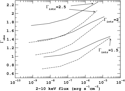
Figure 9: The “$\Gamma_{\rm obs}-F_{\rm 2-10}$” relation for three $\Gamma_{\rm intr}$ values in the case the X–ray continuum varies only in flux, and there exists absorbing material whose ionization parameter varies proportionally with the continuum flux ( solid and dashed lines correspond to N${}_{\rm H}=5\times 10^{22}$ and N${}_{\rm H}=10^{23}$ cm^-2, respectively).

Spectral variations can also be caused by variations in the column density, covering fraction (say $f$), and/or the opacity of an absorber while $\Gamma_{\rm intr}$ remains constant (e.g. Turner et al., 2007; Miller et al., 2008). It is rather unlikely that variations of either the column density or the covering factor are the main driver for the “spectral slope – flux” relation. Under this hypothesis, the N_H or $f$ variations flatten the observed spectral slope and and also reduce the continuum flux, as observed. In other words, in this case the observed flux variations in AGN should not be intrinsic, but they should be caused by the variations in the column density or the covering factor of the absorber. However, many sources in the sample show significant flux variations on time scales as short as a few hundred seconds. Therefore, the continuum flux variability in these objects must be intrinsic to a large extent, as neither N_H nor $f$ are expected to vary on these time scales.

On the other hand, it is possible that the variability of the ionization state of the absorber, due to intrinsic variations of the continuum flux, can affect the spectral shape of the continuum and result in “spectral slope – flux” relations which are similar to the relations we observed: a decrease in the continuum flux will decrease the ionization state of the absorber, increasing its opacity and hence flattening the observed spectrum.

To investigate this possibility we considered the absori*powerlaw model in XSPEC, where absori is an ionised absorption model (Done et al., 1992). The main parameters of this model are the ionisation parameter $\xi$ and the column density, $N_{\rm H}$, of the absorbing medium, as well as $\Gamma_{\rm intr}$ and N_PL, normalisation of the power-law component. We created model spectra assuming $\Gamma_{\rm intr}=1.5$, 2 and 2.5, and various values of N_PL (from 1 up to 5000). We then considered three values of column density, N${}_{\rm H}=10^{22}$, $5\times 10^{22}$ and 10²³ cm^-2 and, for each $\Gamma_{\rm intr}$, we assumed that the ionisation parameter of the absorber is changing proportionally with N_PL (i.e. $\xi\propto$N_PL).

We then used XSPEC to fit a simple PL model to the resulting spectra and determined $\Gamma_{\rm obs}$ and $F_{\rm 2-10}$. In Fig. 9 we plot $\Gamma_{\rm obs}$ as a function of the observed flux for the three $\Gamma_{\rm intr}$ values we considered and in the case when N${}_{\rm H}=5\times 10^{22}$ and N${}_{\rm H}=10^{23}$ cm^-2 (solid and dashed lines, respectively; for simplicity, we assumed, arbitrarily, that $\xi=$N_PL). As expected, the observed spectral slope flattens as the source luminosity decreases. The $\Gamma_{\rm obs}$ change is more pronounced in the case of the absorber with the larger absorbing column (the $\Gamma_{\rm obs}$ variations are of low amplitude in the case of the N${}_{\rm H}=10^{22}$ absorber, and for this reason we do not plot the respective models in Fig. 9).

We fitted the curves shown in Fig. 9 to the data plotted in Fig. 7, by allowing them to shift both in the vertical (i.e. $y_{\rm model}=\Gamma_{\rm obs}+y_{\rm shift}$), and the horizontal direction (i.e. $x_{\rm model}=F_{\rm 2-10}\times x_{\rm shift}$). These model curves fitted well the “$\Gamma_{\rm obs}$ – flux” data of NGC 5548 only. A N${}_{\rm H}=5\times 10^{22}$ cm^-2 absorber whose ionisation parameter varies between $\xi\sim 30-180$, can explain satisfactorily ($\chi^{2}=14.5/8~{}d.o.f.$) the spectral variations we observed in this object. In all other cases, the observed “spectral slope – flux” relations are significantly steeper than any of the model curves plotted in Fig. 9.

We conclude that opacity variations, due to changes in the continuum flux, of a single absorber, whose column density remains constant, cannot explain the observed spectral variations in most AGN in the sample. Of course, if there are multiple layers of absorbing material, the resulting “spectral slope – flux” model curves will be different. However, it is not easy to model such a situation without some apriori knowledge of how many absorbing layers there may be, what their average ionization is, etc.

4.2.3 The case of a constant reflection component

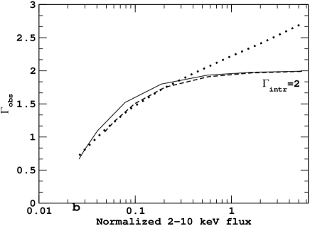
Figure 10: $\Gamma_{\rm obs}$ plotted as a function of $F_{\rm 2-10}$ (normalized to the mean model flux) in the case of a power law with $\Gamma_{\rm intr}=2$ which varies only in normalization and a constant reflection component in the case when the reflecting material is neutral (i.e. $\log(\xi)=0$; solid line) and ionized ($\log(\xi)=3$; dashed line). The dotted line indicates the “spectral slope – flux” relation in the case when $\Gamma_{\rm intr}$ varies with flux ($\Gamma_{\rm intr}\propto F_{\rm 2-10}^{0.08}$) and there also exists a constant reflection component (with $R=1$).

It is possible that the observed spectral variations are due to the combination of a highly variable (in flux) power-law continuum (with $\Gamma_{\rm intr}$=constant) and a constant reflection component (e.g. Taylor, Uttley & M^cHardy, 2003; Ponti et al., 2006; Miniutti et al., 2007). In this case, as the amplitude of the continuum increases, the relative contribution of the reflection component to the observed spectrum will decrease, and $\Gamma_{\rm obs}$ will increase, reaching $\Gamma_{\rm intr}$ when the continuum amplitude is large enough.

To investigate this possibility, we considered a “power-law plus constant reflection” model. To calculate the reflected component we used the pexriv code by Magdziarz & Zdziarski (1995), available in XSPEC. The main model parameters are: (i) the X-ray photon index of the intrinsic power-law, $\Gamma_{\rm intr}$, (ii) the ionisation parameter of the reflecting medium, $\xi$, and (iii) the amplitude of reflection, $R$. We computed model spectra assuming $\Gamma_{\rm intr}=2$, various values of the power law normalization, N_PL (from $3\times 10^{-5}$ up to 0.1), while the normalization of the reflected component, N_refl, was kept fixed (the pexriv model was defined, arbitrarily, so that $|R|=0.1$ and N${}_{\rm refl}=0.1$, where $N_{\rm refl}$ means normalization of the power-law continuum that is reflected). Since the power-law was defined explicitly in our model, we used pexriv with $R<0$, which outputs only the reflected component.

We then used XSPEC to fit a power-law to the model spectra in the 2–10 keV band and determined model $\Gamma_{\rm obs}$. In Fig. 10 we plot $\Gamma_{\rm obs}$ as a function of the total 2–10 keV flux (normalized to the mean model flux) in the case when the reflecting material is neutral (i.e. $\log(\xi)=0$; solid line) and ionized ($\log(\xi)=3$; dashed line), and the slope of the power law is fixed at $\Gamma_{\rm intr}=2$. As expected, as the flux decreases, the relative strength of the reflecting component increases, and $\Gamma_{\rm obs}$ becomes harder.

The shape of the model curves in the case of different $\Gamma_{\rm intr}$ values is identical to the ones shown in Fig. 10 except for the fact that, in the high flux limit, they saturate at their respective $\Gamma_{\rm intr}$ value. Similarly, the shape of the model curves remains the same if we increase the total flux while keeping the relative strength of the power-law and the reflection component (and hence $\Gamma_{\rm obs}$) the same. As a result the curves will only shift to a higher flux.

We fitted the curves shown in Fig. 10 to the data plotted in Fig. 7 by allowing them to shift both in the vertical (i.e. $y_{\rm model}=\Gamma_{\rm obs}+y_{\rm shift}$), and the horizontal direction (i.e. $x_{\rm model}=F_{\rm 2-10,mod}\times x_{\rm shift}$; $F_{\rm 2-10,mod}$ is the model 2–10 keV flux). The shift along the $y-$axis is necessary because $\Gamma_{\rm intr}$ may not be equal to 2 in all objects. The best fit vertical offset value, $y_{\rm bf}$, will determine the best fit intrinsic slope for each object, $\Gamma_{\rm intr}=2+y_{\rm bf}$. On the other hand, the horizontal offset shift is necessary, given the different flux levels of the objects, and the fact that the strength of the reflection component in each object, with respect to that of the power-law continuum (i.e. the average $R$ in each object, $\overline{R}$), is not known apriori. In fact, the best fit horizontal offset value, $x_{\rm bf}$, can be used to determine $\overline{R}$ as follows.

The reflection amplitude, $R$, determines the fraction of the X–ray photons that are reflected by the disc, so that $R\propto F_{\rm refl}/F_{\rm PL}$ (where $F_{\rm refl}$ and $F_{\rm PL}$ are the fluxes of the reflected component and continuum, respectively). In our case, the average source flux, $\overline{F}_{\rm 2-10,obs}$, corresponds to a model PL flux of $F_{\rm PL,mod}=(\overline{F}_{\rm 2-10,obs}/x_{\rm bf})-F_{\rm refl,mod}$. The model curve was constructed by assuming, arbitrarily, the constant reflection component when $R=0.1$ and N${}_{\rm PL}=0.1$, therefore $\overline{R}=0.1\times F_{\rm PL,mod}(0.1)/F_{\rm PL,mod}$, where $F_{\rm PL,mod}(0.1)$ is the 2–10 keV flux of the power law with N${}_{\rm PL}=0.1$.

The model curves plotted in Fig. 10 fitted well the data of all objects, except for NGC 3227 ($\chi^{2}=55.1/8~{}d.o.f.$), NGC 5506 ($\chi 2=22.2/8~{}d.o.f.$), and NGC 5548 ($\chi 2=40.4/8~{}d.o.f.$). In the case of MCG -6-30-15 and NGC 3516 it was reflection from ionized material that fitted the data best. We plot the “$\Gamma_{\rm obs}-F_{\rm 2-10}$” data for the objects in the sample in Fig. 11. Best fit lines are indicated by the solid lines.

The best model fits do not provide a statistically acceptable fit to the data of NGC 3227, NGC 5506, and NGC 5548. In the case of NGC 5548, the model describes rather well the “$\Gamma_{\rm obs}-$flux” data, except for the lowest flux point (the best fit model line plotted in Fig. 11 for NGC 5548 corresponds to reflection from ionized material). The disagreement between best model fit and data points is more pronounced in the case of NGC 3227, especially at low fluxes. This is a source where a possible absorption event, which lasted for a few months, has been observed in its RXTE light curve (Lamer, Uttley & M^cHardy, 2003). In this case, one would expect $\Gamma_{\rm obs}$ to be harder than the model predictions at a given (low) flux, which is opposite to what is observed. However, such an event should also shift the model line to lower fluxes. Therefore it is difficult to reach final conclusions regarding the quality of the model fit to the NGC 3227 data.

The best fit intrinsic spectral slopes ranged from $\Gamma_{\rm intr}\sim 1.8$ in NGC 5548, to $\Gamma_{\rm intr}\sim 2.8$ in Ark 564. Furthermore, the best fit $x_{\rm bf}$ values imply large average $R$ values: from $\overline{R}\sim 0.5$ in the case of NGC 5548 up to $\overline{R}\sim 15$ in the case of NGC 3516. The median $\overline{R}$ is 4.7. We did not detect any correlation between the resulting best-fit $\Gamma_{\rm intr}$ and $\overline{R}$ values.

The reflection amplitude $R$ is essentially equal to the solid angle covered by the reflecting material and is equal to 1 in the case of a point source on top of a disc at large heights (i.e. in the case when $\Omega=2\pi$). Values as large as $R\sim 5$ suggest either a peculiar geometry (which is difficult to envisage) or non-isotropic emission from the X–ray continuum in which case the X–ray flux on the reflecting material is much larger than the flux which reaches the observer (see e.g. Miniutti & Fabian, 2004, for the case of an X–ray source which is located very close to a rapidly rotating black hole, in which case relativistic light bending effects are important).

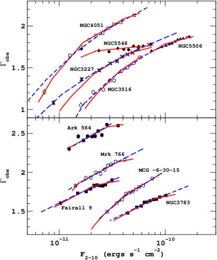
Figure 11: The $\Gamma_{\rm obs}-F_{\rm 2-10}$ relations for the objects in the sample together with the best fit curves for the models described in sections 4.2.3 (solid line) and 4.2.4 (dashed line).

4.2.4 The case of $\Gamma_{\rm intr}$ variations plus a constant reflection component

.

We considered next the possibility that the X–ray continuum in AGN consists of a constant reflection component and a power-law continuum with variable N_PL and $\Gamma_{\rm intr}$. This is a combination of the two cases we considered above: X–rays are produced by thermal Comptonization, the flux variations (i.e. the N_PL variations) reflect intrinsic variations in the accretion rate, and $\Gamma_{\rm intr}=2.7\dot{m}^{0.08}$ (this is the best power-law model fit to the $\Gamma_{\rm intr}-\dot{m}$ relation plotted in Fig. 5c). The X–ray source illuminates a reflecting material, which effectively responds to the average X–ray continuum (i.e. to a power-law of $\sim\overline{\Gamma}_{\rm intr}$ and $\overline{{\rm N}}_{\rm PL}$). This could be for example the case of a reflector which is located away from the X–ray source.

To investigate this possibility, we considered again the model pexriv+powerlaw in XSPEC. This time, we created model spectra assuming 8 values of the power law normalization (from $10^{-4}$ up to 0.1) and a spectral slope of $\Gamma_{\rm intr}=2.7$N${}_{\rm PL}^{0.08}$ (the arbitrary choice $\dot{m}=$N_PL was made for simplicity; it does not affect our results, as long as the resulting model curves are allowed to shift freely along the $x-$axis when we fit them to the data). Then, for each pair of values (N${}_{\rm PL},\Gamma_{\rm intr})$ we considered the respective reflection component (from neutral material) in the case when $R=1$, and we added it to all 8 power-law spectra. In this way, we constructed 8 sets of model curves (8 model spectra in each set).

We then used XSPEC to fit a simple PL model to the 8 spectra of each model set and determined $\Gamma_{\rm obs}$ and the spectrum flux in the 2–10 keV band ($F_{\rm 2-10}$). The dotted line in Fig. 10 indicates $\Gamma_{\rm obs}$ in the case when we added to all 8 spectra the reflection component (with $R=1$) from a $\overline{\Gamma}_{\rm intr}=2$ power-law continuum, plotted as a function of $F_{\rm 2-10}$ (normalized to the mean model flux).

We fitted the 8 “$\Gamma_{\rm obs}$ – $F_{\rm 2-10}$” model curves to the observed “spectral slope – luminosity” relations plotted in Fig. 7 by allowing them to shift both in the vertical (i.e. $y_{\rm model}=\Gamma_{\rm obs}+y_{\rm shift}$), and the horizontal direction (i.e. $x_{\rm model}=x_{\rm shift}\times F_{\rm 2-10,mod}$). These model curves fitted well the “$\Gamma-\dot{m}$” data of all objects, except for NGC 4051 and NGC 5548.

The dashed lines in Fig. 11 indicate the best fit curves for this model. Interestingly, the model fits well the NGC 3227 data, a result which implies that the flat $\Gamma_{\rm obs}$ at low fluxes may correspond to intrinsically flatter spectra, and not an increase in the external absorption by cold gas. In the case of NGC 4051, the fit is not statistically acceptable ($\chi^{2}=20.9/8~{}d.o.f.$, $p_{\rm null}=7.4\times 10^{-3}$) mainly because of the lowest flux point. Furthermore, the model fails entirely to describe the NGC 5548 data. This result is obvious given the fact that the model curves in this case have no flat part that could fit, even approximately, the observed NGC 5548 data.

In principle, we should not allow a $y-$axis shift of the model curves in this case. The intrinsic spectral slope is uniquely determined by the $\Gamma_{\rm intr}-$N_PL relation we assumed. However, the assumed relation was determined by the PL model fit to the “average spectral slope - average accretion rate” data plotted in Fig. 5c, hence there is an uncertainty associated with its normalization and slope. The average best fit $y-$axis shift for all objects is 0.13$\pm 0.08$, i.e. it is consistent with zero. This result implies that the relation $\Gamma_{\rm intr}\sim 2.7\dot{m}^{0.08}$ is in agreement with both the average “spectral slope - accretion rate” relation of all objects and with the individual “slope - luminosity” relations of each AGN.

The Ark 564 data are fitted best in the case when the constant reflection component is the one which corresponds to $\overline{\Gamma}_{\rm intr}=2.45$. The Mrk 766 and NGC 4051 data are fitted best in the case of constant reflection component for $\overline{\Gamma}_{\rm intr}=2.25$ and 1.9, respectively. In all other cases, the addition of a constant component for $\overline{\Gamma}_{\rm intr}=1.7$ is needed to fit the data best.

5 Conclusions

We analyzed more than 7,500 RXTE PCA data of 10 nearby AGN with the goal of studying their spectral variability properties. The objects were observed regularly with RXTE over many years since 1996. Given the large number of observations, spread over many years, we were able to determine accurately their average observed spectral slope, luminosity and accretion rate. Using the best model-fit results from the hundreds of spectra of each source, we also determined their long-term “observed spectral slope – X–ray flux” relation. This kind of long term variability analysis can not be accomplished with the rather short AGN observations currently performed by Chandra, XMM-Newton or Suzaku, despite their higher effective area and superior spectral resolution. Our main results are as follows:

• The average spectral slope is not the same in all objects. It does not correlate either with BH mass or luminosity. However, $\overline{\Gamma}$ correlates positively with the mass accretion rate: objects with higher accretion rate have steeper spectra, and $\Gamma\simeq 2.7\dot{m}^{0.08}$. This result can be explained if the Compton amplification factor, $A$, decreases proportionally with the accretion rate in AGN.

• We detected the iron K$\alpha$ line in many spectra of seven sources in the sample. The average EW of the line anti-correlates with the average 2–10 keV luminosity (i.e. the so-called Iwasawa-Taniguchi effect). Our results are in agreement with recent results which are based on recent studies of large samples of AGN (Bianchi et al., 2007).

• The spectra of each source become steeper with increasing flux. This is a well known result. What we have shown in this work that this trend holds over many years, and over almost the full range of flux variations that AGN exhibit. We also found that the $\Gamma_{\rm obs}-F_{\rm 2-10}$ relations are similar in all objects, except for NGC 5548. There are many reasons which can cause apparent and/or intrinsic variations in the X–ray spectrum of AGN. It is possible that they all operate, to a different extent in various objects. However, the common spectral variability pattern we detected implies that just a single mechanism is responsible for the bulk of the observed spectral variations.

• NGC 5548 displays limited spectral variations for its flux variability. Although uncommon, this behaviour has also been observed in other Type I Seyfert, PG 0804+761 (Papadakis, Reig & Nandra, 2003). This behaviour, different to what is observed in most (Type I) AGN, raises the issue of different spectral states in AGN, just like in GBHs. Investigation of this issue is beyond the scope of the present work.

• The scenario in which the spectral variability is caused by absorption of X-rays by a single medium whose ionization parameter varies proportionally to the continuum flux variations fails to account for the observed spectral variations.

• A “power-law, with constant $\Gamma_{\rm intr}$ and variable flux, plus a constant reflection component” can fit the observed “$\Gamma-F_{\rm 2-10}$” relations of most (but not all) objects in the sample. The flux of the reflection component necessary to explain the observed spectral variability is rather large, implying average reflection amplitudes of the order of $R\sim 5$. If true, this result implies that the primary source of X-rays is located close to a maximally rotating Kerr black hole, where relativistic effects (such as light bending) are expected to be strong.

• The observed “$\Gamma-F_{\rm 2-10}$” relations (except for NGC 5548) can be explained if we assume that the power-law continuum varies both in flux and shape as $\Gamma_{\rm intr}\propto F_{\rm 2-10}^{0.08}$ (as implied by the average “spectral slope - accretion rate” relation that we observed) and the reflecting material responds to the average continuum spectrum, with $R=1$.

References

- Arnaud (1996) Arnaud K.A., 1996, Astronomical Data Analysis Software and Systems V, 101, 17
- Beloborodov (1999) Beloborodov A.M., 1999, High Energy Processes in Accreting Black Holes, 161, 295
- Bian (2005) Bian W.H., 2005, CHJAA, 5, 289
- Bianchi et al. (2007) Bianchi S., Guainazzi M., Matt, G., Fonseca Bonilla N., 2007, A&A, 467, L19
- Botte et al. (2004) Botte V., Ciroi S., Rafanelli P. & Di Mille F., 2004, AJ, 127, 3168
- Coppi (1999) Coppi P.S., 1999, High Energy Processes in Accreting Black Holes, 161, 375
- Done et al. (1992) Done C., Mulchaey J.S., Mushotzky R.F., Arnaud K.A., 1992, ApJ, 395, 275
- Esin et al. (1997) Esin A.A., McClintock J.E., Narayan R., 1997, ApJ, 489, 865
- Fabian & Vaughan (2003) Fabian A.C., Vaughan S., 2003, MNRAS, 340, L28
- Greene & Ho (2005) Greene J.E. & Ho L.C., 2005, ApJ, 627, 721
- Haardt et al. (1997) Haardt F., Maraschi L., Ghisellini G., 1997, ApJ, 476, 620
- Iwasawa & Taniguchi (1993) Iwasawa K., Taniguchi Y., 1993, ApJL, 413, L15
- Jahoda et al. (1996) Jahoda K., Swank J.H., Giles A.B., Stark M.J., Strohmayer T., Zhang W., Morgan E.H., 1996, Proc. SPIE, 2808, 59
- Lamer et al. (2003) Lamer G., Uttley P., McHardy I.M., 2003, MNRAS, 342, L41
- Magdziarz & Zdziarski (1995) Magdziarz P., Zdziarski A.A., 1995, MNRAS, 273, 837
- Malzac et al. (2001) Malzac J., Beloborodov A.M., Poutanen J., 2001, MNRAS, 326, 417
- McHardy et al. (2005) McHardy I.M., Gunn K.F., Uttley P. & Goad M.R., 2005, MNRAS, 359, 1469
- McHardy et al. (2006) McHardy I.M., Koerding E., Knigge C., Uttley P., Fender R.P., 2006, Nature, 444, 730
- Miller et al. (2008) Miller L., Turner T.J., Reeves J.N., 2008, A&A, 483, 437
- Miniutti & Fabian (2004) Miniutti G. & Fabian A.C., 2004, MNRAS, 349, 1435
- Miniutti et al. (2007) Miniutti G. et al., 2007, PASJ, 59, 315
- Nandra & Papadakis (2001) Nandra K. & Papadakis I.E., 2001, ApJ, 554, 710
- Papadakis et al. (2002) Papadakis I.E., Petrucci, P.O., Maraschi L., McHardy I.M., Uttley P., Haardt F., 2002, ApJ, 573, 92
- Papadakis et al. (2003) Papadakis I.E., Reig P., Nandra P., 2003, MNRAS,344, 993
- Papadakis et al. (2009) Papadakis I.E., Sobolewska M., Arevalo P., Markowitz A., McHardy I.M., Miller L., Reeves J.N., Turner T.J., 2009, A&A, 494, 905
- Perola et al. (2002) Perola G.C., Matt G., Cappi M., Fiore F., Guainazzi M., Maraschi L., Petrucci P.O. & Piro L., 2002, A&A, 389, 802
- Peterson et al. (2004) Peterson B.M. et al., 2004, ApJ, 613, 682
- Ponti et al. (2006) Ponti G., Miniutti G., Cappi M., Maraschi L., Fabian A.C., Iwasawa K., 2006, MNRAS, 368, 903
- Porquet et al. (2004) Porquet D., Reeves J.N., O’Brien P., Brinkmann W., 2004, A&A, 422, 85
- Reeves et al. (2004) Reeves J.N., Nandra K., George I.M., Pounds K.A., Turner T.J., Yaqoob T., 2004, ApJ, 602, 648
- Saez et al. (2008) Saez C., Chartas G., Brandt W.N., Lehmer B.D., Bauer F.E., Dai X., Garmire G.P., 2008, AJ, 135, 1505
- Shemmer et al. (2006) Shemmer O., Brandt W.N., Netzer H., Maiolino R., Kaspi S., 2006, ApJL, 646, L29
- Taylor et al. (2003) Taylor R.D., Uttley P., McHardy I.M., 2003, MNRAS, 342, L31
- Tremaine et al. (2002) Tremaine S. et al., 2002, ApJ, 574, 740
- Turner et al. (2007) Turner T.J., Miller L., Reeves J.N., Kraemer S.B., 2007, A&A, 475, 121
- Turner & Miller (2009) Turner T.J., Miller L., 2009, A&ARv, 17, 47
- Vaughan et al. (2003) Vaughan S., Edelson R., Warwick R.S., Uttley P., 2003, MNRAS, 345, 1271
- Wang & Zhang (2007) Wang J.M. & Zhang E.P., 2007, ApJ, 660, 1072
- Wu & Gu (2008) Wu Q., Gu M., 2008, ApJ, 682, 212
- Zdziarski et al. (1999) Zdziarski A.A., Lubiński P., Smith D.A., 1999, MNRAS, 303, L11
- Zhang & Wang (2006) Zhang E.P. & Wang J.M., 2006, ApJ, 653, 137