Adiabatic evolution under quantum control
Abstract
One of the difficulties in adiabatic quantum computation is the limit on the computation time. Here we propose two schemes to speed-up the adiabatic evolution. To apply this controlled adiabatic evolution to adiabatic quantum computation, we design one of the schemes without any prior knowledge of the instantaneous eigenstates of the final Hamiltonian. Whereas in another scheme, the control is constructed with the instantaneous eigenstate that is the target state of the control. As an illustration, we study a two-level system driven by a time-dependent magnetic field under the control. The physics behind the control scheme is explained.
pacs:
03.65.-w, 03.65.Ta, 02.30YyAdiabatic quantum computation (AQC) was first proposed in 2000Farhi01 as a means to solve NP-complete problems. It is polynomially equivalent to conventional (gate model) quantum computationadkllr04 and possesses some degree of fault tolerance. AQC can be described by the following Hamiltonian,
| (1) |
where the quantum system govern by evolves slowly with time and remains in its ground state as changes monotonically from 0 to 1 within a time . The initial Hamiltonian is assumed to have an easily accessible ground state into which the system is initialized, while the ground state of the final Hamiltonian encodes a problem’s solution. In order to reach the final ground state with high fidelity, the adiabatic theorem requires , where is the minimum gap between the two lowest energy eigenstates of . The power can be 1, 2, or possibly some other number depending on the functional form of and the distribution of the higher energy levels Farhi01 ; schaller06 ; lidar08 . This leads to a limit on the computation time , which holds true for adiabatic quantum computation without quantum control, thus it is natural to ask whether one can use quantum control to speed up AQC?
Quantum controllloyd00 ; viola98 ; ramakrishna95 ; schirmer01 ; wiseman94 ; mancini98 ; belavkin99 ; doherty99 ; carvalho07 ; yi08 is about the application of classical and modern control strategy to quantum systems. It has generated increasing interest in the last few years due to its potential applications in metrologywiseman95 ; berry01 , communicationsgeremia04a ; jacobs07 and other technologies ahn02 ; hopkins03 ; geremia04b ; sarovar04 ; steck04 , as well as its theoretical interest on its own. Several approaches to the control of a quantum system have been proposed in the past decade, which can be divided into coherent (unitary) and incoherent (non-unitary) control, according to how the controls enter the dynamics. In the coherent control scheme, the controls enter the dynamics through the system Hamiltonian. It affects the time evolution of the system state, but not its spectrum, i.e., the eigenvalues of the target density matrix remain unchanged in the dynamics. In the incoherent control scheme, an auxiliary system, called probe, is introduced to manipulate the target system through their mutual interaction. This incoherent control scheme is of relevance whenever the system dynamics can not be directly accessed and provides a non-unitary evolution for the quantum system. This breaks the limitation for the coherent control mentioned above. Among these quantum control strategies, Lyapunov control plays an important role in quantum control theory. Lyapunov functions, originally used in control to analyze the stability of the control system, have formed the basis for new control design. Several papers have be published recently to discuss the application of Lyapunov control to quantum systemsvettori02 ; ferrante02 ; grivopoulos03 ; mirrahimi04 ; mirrahimi05 ; altafini07 ; wang08 ; yi09 . Although the basic mathematical formulism for Lyapunov control is well established, many questions remain when one considers its applications in quantum information processing, for instance, whether one can use quantum Lyapunov control to improve the adiabatic evolution, and consequently minimize the computation time?
In this paper, we shall address this issue by using a two-level model with Lyapunov control. Since the two lowest levels are important for AQC, this model to some extent can good quantify the AQC under control. Two control schemes are proposed which correspond to two different choices of Lyapunov function. By numerical simulation, we find that these schemes work well. The paper is organized as follows. In Sec.II, we present a general formalism for the Lyapunov control, two Lyapunov functions which will give two control schemes are constructed, then we use these schemes to manipulate a two-level system in Sec.III. Conclusion and discussions are presented in Sec.IV.
General formalism.— Let us start by focusing on the Hamiltonian in Eq.(1). We denote the instantaneous eigenstates and the corresponding eigenvalues of by and , respectively. AQC is designed to take advantage of the adiabatic theorem, it works by evolving a system from the accessible ground state of an initial Hamiltonian to the ground state of a final Hamiltonian For the system to remain in its ground state, the adiabatic theorem requires that the system Hamiltonian changes very slowly and there is an energy gap between the ground state and the others. The goal of this paper is to manipulate the system such that it remains in one of its eigenstates. To meet the requirement of AQC, any information about the instantaneous eigenstates of is forbidden to use in the control, but a prior knowledge regarding the system Hamiltonian is allowed. This motivates us to propose the first scheme in the following. Beside the interests in AQC, controlling a quantum system to a target state is interesting on its own. As the target state is known, the information about the target state can be used in the control design. This is the goal of the second scheme discussed in this paper.
Scheme A.— We aim to design a control scheme that can manipulate a system to remain in its instantaneous ground state without any prior knowledge of its instantaneous eigenstates of . To this end, we introduce control operators and require that for any The control operators enter the system through control field The total Hamiltonian of the system is then written,
| (2) |
where the control field can be established by Lyapunov control theory. Define a function as
| (3) |
with being a time-independent Hermitian operator, we find and
| (4) |
Here and hereafter denotes the state of the system that satisfy We now show how to establish the control field . Lyapunov control theory tells that for to be a Lyapunov function, has to satisfy, and So, if we choose the control field as
| (5) |
then Here was specified to satisfy Clearly is a time-dependent real number, thus the total Hamiltonian is Hermitian. The key point of this control scheme is the choice of operator it dominates the success rate of the control and show the merit in this scheme. From the control design of the scheme, we find that the instantaneous eigenstates do not enter the control, this mean that by the present control strategy, we can manipulate the quantum system to evolve along one of the eigenstates without any knowledge of its instantaneous eigenstates. This is exactly what we want in AQC. To see that this control scheme indeed works, we note that indicating the control itself can not induce population transfer among the instantaneous eigenstates. Suppose that the system is initially prepared in its ground state and , Eq.(5) yields and regardless of what takes. When deviates from , can be very large depending on operator . The Lyapunov control will then render the system nonlinear, and this nonlinear effect would bring the state back to We note that (as well as can derive the system from one instantaneous eigenstate to the others, this together with the control keep the system in the instantaneous eigenstate into which the system was initially prepared. We will demonstrate this point through an example in detail later.
Scheme B.—For general control problem, the target state is known, we then can use the target state to design a Lyapunov function and establish the control field Suppose that the target state is the zeroth instantaneous eigenstate of , define
| (6) |
Clearly with equality only if To see Eq.(6) indeed defines a Lyapunov function, we calculate the time derivative of as( in this scheme),
| (7) | |||||
Obviously,
| (8) |
guarantee that Again, was selected to satisfy Hence, the evolution of the system with Lyapunov control can be described by the following nonlinear autonomous equations,
| (9) |
where are given by Eq.(8). Note that is not required in this scheme. The difference between the present scheme and those in the literaturewang08 is the target state. In earlier studies, the target state is either time-independent or time-dependent via , whereas in our scheme, the target state is one of the instantaneous eigenstate of . The time derivative of the instantaneous eigenstate plays an important role in the control, leading to totally different control fields in Eq.(8). Note that the choice of in Eqs.(5) and (8) are not unique. In fact, when there is only one control operator , the control field in Eq.(5) can be chosen as,
| (10) | |||||
provided is a finite number. This is exactly the case in the example that we will illustrate below.
Example.— As an illustration of the Lyapunov control scheme, we discuss below a two-level system driven by a time-dependent magnetic field. The Hamiltonian that describes such a system can be written as
where and are the Pauli matrices, is the amplitude of the classical field. is specified to be a constant here, while depends on time through (, constant). In comparison with Eq.(1), takes while . Although in this model we can not found an analytical by which we write Eq.(Adiabatic evolution under quantum control) in the form of Eq.(1), the model Eq.(Adiabatic evolution under quantum control) can be obviously mapped into Eq.(1). It is well know that the instantaneous eigenstates and the corresponding eigenvalues of are and , respectively.
In the absence of Lyapunov control, it is required that for the system to evolve adiabatically. We now show that the system can evolve along one of its instantaneous eigenstates, e.g. , under the Lyapunov control even if In the following, a fidelity defined by
| (12) |
will be used to measure the effectiveness of the control. The dependence of on time and the control operator as well as are shown. The results show that these schemes work good with properly chosen and .
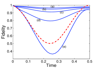
We first consider the scheme A, where no information about instantaneous eigenstates enter the control. Choose with a rate , the dynamics of the two-level system under control is governed by
| (13) | |||||
Here was specified to be in order to satisfy We have perform extensive numerical simulations for the dynamics Eq.(13), selected results are plotted in Fig. 1. Two observations can be found from Fig.1. (1) The scheme works only for special . For some choices of , the control favors the adiabatic evolution, but for the other , the control spoils the adiabaticity of the evolution. (2) For the specified , , the larger the ratio is, the better the fidelity for the system in .
In the scheme B, a prior knowledge of the instantaneous eigenstates is known and allowed to use to design the control field . Choose as the target state, the dynamics of the system is governed by Eq.(9) with replacing by . We show in Fig.2 the fidelity as a function of time with
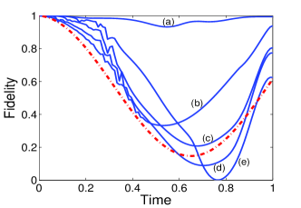
Similar to the results given in the scheme A, the choice of the control operator dominates the effectiveness of the control. Not all control operator can help the adiabatic evolution. The difference between these two scheme is that the scheme B can reach fidelity 1 at the final stage, this may depend on the example demonstrated.
For linear quantum system, the population transfer from one instantaneous eigenstate to the others depends on the energy gap and the operator that induces the transfer. The energy gap separates the instantaneous eigenstates and ensures the adiabaticity of the evolution. The larger the energy gap is, the higher the probability with which the system remains in the instantaneous eigenstate. In the scheme A, the operator that induces the population transfer is small would benefits the adiabaticity of the system. For nonlinear system, however, the nonlinearity plays an important role in addition to the factors for linear system mentioned above. All these factors together lead to the observed features and can be used to understand the physics behind the features.
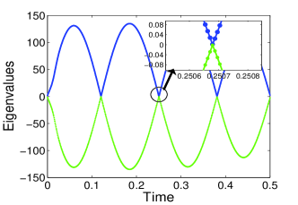
To make the explanation clear, we plot the eigenvalues for the total Hamiltonian in scheme A as a function of time in Fig.3. The same parameters as in Fig.1-(a) are chosen, which ensure that the state of the system remains in the instantaneous eigenstate . Recall that the energy gap between two instantaneous eigenstates is 2 (in units of ) for , we find from Fig.3 that the energy gap is intensively enlarged at most times by the control. Nevertheless, the enlarged energy gap itself can not explain why the system remains well in the instantaneous eigenstate, because the energy gap is very small at the level anti-crossing points, this indicates that the nonlinearity must play an important role in the dynamics. Indeed our numerical calculation shows that at these point, the nonlinear coefficient defined by is much larger than the tunneling coefficient leading to the observed feature reminiscent of self-trapping in nonlinear system.
To sum up, we have proposed two schemes to speed-up the adiabatic evolution. In the scheme A, the control has been designed without any information about the instantaneous eigenstates of the final Hamiltonian, hence this scheme can be used in the adiabatic quantum computation. The scheme B has been proposed using the instantaneous eigenstate of the system Hamiltonian. This scheme is applicable to control a quantum system when the target state is known. To show how the schemes work, we have presented an example consisting of a two-level system in a rotating magnetic field. The fidelity to quantify the effectiveness of the scheme was calculated and discussed. The results show that the fidelity depends sharply on the choice of and the control operator . The physics behind the schemes is revealed, which can be understood as an effect combining nonlinear effects and the broadened energy gap.
This work was supported by NSF of China under grant Nos. 10775023 and 10935010.
References
- (1) E. Farhi, J. Goldstone, S. Gutmann, J. Lapan, A. Lundgren, and D. Preda, Science 292, 472 (2001).
- (2) D. Aharonov, W. van Dam, J. Kempe, Z. Landau, S. Lloyd, and O. Regev, Proc. 45th FOCS, 42 (2004).
- (3) G. Schaller, S. Mostame, and R. Schützhold Phys. Rev. A 73, 062307 (2006).
- (4) D.A. Lidar, A.T. Rezakhani, and A. Hamma, eprint arXiv:0808.2697.
- (5) S. Lloyd, Phys. Rev. A 62, 022108(2000).
- (6) L. Viola and S. Lloyd, Phys. Rev. A 58, 2733(1998); L. Viola, E. Knill, and S. Lloyd, Phys. Rev. Lett 82, 2417(1999).
- (7) V. Ramakrishna, M. V. Salapaka, M. Dahleh, H. Rabitz, A. Peirce, Phys. Rev. A 51, 960(1995).
- (8) S. G. Schirmer, H. Fu, and A. I. Solomon, Phys. Rev. A 63, 063410(2001); H. Fu, S. G. Schirmer, and A. I. Solomon, J. Phys. A 34, 1679(2001).
- (9) H. W. Wiseman and G. J. Milburn, Phys. Rev. Lett. 70, 548(1993); H.M.Wiseman, Phys. Rev. A 49, 2133(1994).
- (10) S. Mancini, D. Vitali, and P. Tombesi, Phys. Rev. Lett. 80, 688(1998).
- (11) V. P. Belavkin, Rep. Math. Phys. 43, 405(1999).
- (12) A. C. Doherty and K. Jacobs, Phys. Rev. A 60, 2700(1999).
- (13) A. R. R. Carvalho, J. J. Hope, Phys. Rev. A 76, 010301(R)(2007).
- (14) L. C. Wang, X. L. Huang, and X. X. Yi, Phys. Rev. A 78, 052112 (2008); H. Y. Sun, P. L. Shu, C. Li, and X. X. Yi, Phys. Rev. A 79, 022119 (2009).
- (15) H. M. Wiseman, Phys. Rev. Lett. 75, 4587(1995).
- (16) D. W. Berry, H. M. Wiseman,and J. K. Breslin, Phys. Rev. A 63 053804,(2001).
- (17) K. Jacobs, Quant. Information Comp.7, 127(2007).
- (18) J. M. Geremia, Phys. Rev. A 70, 062303(2004).
- (19) C. Ahn, A. C. Doherty, and A. J. Landahl, Phys. Rev. A 65, 042301(2002).
- (20) A. Hopkins, K. Jacobs, S. Habib, and K. Schwab, Phys. Rev. B 68, 235328(2003).
- (21) M. Sarovar, C. Ahn, K. Jacobs, and G. J. Milburn, Phys. Rev. A 69, 052324 (2004).
- (22) D. A. Steck, K. Jacobs, H. Mabuchi, T. Bhattacharya, and S. Habib, Phys. Rev. Lett.92, 223004(2004).
- (23) M. A. Armen, J. K. Au, J. K. Stockton, A. C. Doherty, and H. Mabuchi, Phys. Rev. Lett. 89, 133602 (2002).
- (24) P. Vettori, in Proceedings of the MTNS Conferene, 2002.
- (25) A. Ferrante, M. Pavon, and G. Raccanelli, in Proceedings of the 41st IEEE Conference on Decision and Control, 2002.
- (26) S. Grivopoulos and B. Bamieh, in Proceedings of the 42nd IEEE Conference on Decision and Control, 2003.
- (27) M. Mirrahimi and P. Rouchon, in Proceedings of IFAC Symposium LOLCOS 2004; In Proceedings of the International Symposium MTNS 2004.
- (28) M. Mirrahimi and G. Turinici, Automatica 41, 1987(2005).
- (29) C. Altafini, Quantum Information Processing 6, 9(2007).
- (30) X. Wang and S. Schrimer, arXiv: 0801.0702; arXiv: 0901.4515.
- (31) X. X. Yi, X. L. Huang, Chunfeng Wu, and C. H. Oh, arXiv:0908.1048, Phys. Rev. A, accepted.