Entanglement creation between two causally-disconnected objects

Abstract

We study the full entanglement dynamics of two uniformly accelerated Unruh-DeWitt detectors with no direct interaction in between but each coupled to a common quantum field and moving back-to-back in the field vacuum. For two detectors initially prepared in a separable state our exact results show that quantum entanglement between the detectors can be created by the quantum field under some specific circumstances, though each detector never enters the other’s light cone in this setup. In the weak coupling limit, this entanglement creation can occur only if the initial moment is placed early enough and the proper acceleration of the detectors is not too large or too small compared to the natural frequency of the detectors. Once entanglement is created it lasts only a finite duration, and always disappears at late times. Prior result by Reznik Reznik03 derived using the time-dependent perturbation theory with extended integration domain is shown to be a limiting case of our exact solutions at some specific moment. In the strong coupling and high acceleration regime, vacuum fluctuations experienced by each detector locally always dominate over the cross correlations between the detectors, so entanglement between the detectors will never be generated.

I Introduction

Quantum entanglement, the uniquely quantum mechanical feature of a quantum system as Schrödinger emphasized Sc35 , is the distinguishing resource of quantum information processing (QIP). Its evolutionary behavior in time is thus of primary importance to the viability and functioning of quantum computing. Many QIP candidate systems involve qubits interacting with a quantum field, such as two level atoms (2LA) in a cavity. Because of the intrinsically relativistic nature of a quantum field, in that physical information propagates at a finite speed, issues of causality are unavoidably imbued with QIP, even though the qubits in popular schemes are likely to move at nonrelativistic speed or remain stationary. It is of interest to ask whether quantum entanglement can transcend such limitations. This underlies the frequently mentioned yet often-misconjured notion of “quantum nonlocality” such as usually associated with the famous EPR paper EPR .

Following our two recent work discussing the behavior of quantum entanglement in a relativistic setting, one with a detector (an object with internal degrees of freedom such as a harmonic oscillator or an atom) in relativistic motion LCH2008 and another focusing on the relativistic features of a quantum field mediating two inertial detectors LH2009 in this paper we study the conditions whereby quantum entanglement between two causally disconnected detectors (spacelike separated, outside of each other’s light cone) can be created and if so how it evolves in time. By pushing to extreme conditions we can appreciate better this unique feature of quantum mechanics assessed in the more complete setting of relativistic quantum fields.

The question in focus here is, whether quantum entanglement between two localized causally disconnected atoms can be created by the vacuum of a common mediating quantum field they both interact with, but not directly with each other. Refs. Reznik03 ; RRS05 ; MS06 ; Franson08 affirm such a possibility whereas Refs. Braun05 ; LH2009 see no such evidence. These are not contradictory claims because the setups of the problem are not exactly the same.

Using the time-dependent perturbation theory (TDPT) with extended integration domain, Reznik discovered that a pair of two-level atoms initially in their ground states will become entangled when they are uniformly accelerated back-to-back in the Minkowki vacuum of the field, even though in this setup the two atoms are causally disconnected Reznik03 . Later Massar and Spindel (MS) MS06 considered an exactly solvable model with two Unruh-Raine-Sciama-Grove (U-RSG) harmonic oscillators RSG91 moving in a similar fashion in (1+1) dimensions but both in equilibrium with the Minkowski vacuum. They discovered that entanglement can indeed be created, but only in a finite duration of Minkowski time after the moment that the distance between the detectors is the minimum. However, contrary to Reznik’s perturbative results, MS found that such entanglement creation process does not occur in perturbative regime. In our assessment, since MS were looking at the late-time steady-state behavior (where “the detectors are in equilibrium with the Unruh heat bath” MS06 ), their result cannot be compared with Reznik’s TDPT result, which corresponds to early-time behavior of the detectors or atoms.

To resolve the difference and understand the discrepancy our present investigation adopts the physical system used in LH2009 to a situation similar to that considered in Reznik03 or MS06 . Taking advantage of the existence of exact solutions to the model under study we can perform a thorough analysis and follow the system’s evolution through their whole history which enables us to identify the conditions (in the motion of the two atoms), the approximations invoked (e.g., time dependent perturbation theory used in Reznik03 ) and the parameter ranges where quantum entanglement may be generated.

This paper is organized as follows. In Sec. II we introduce the model and describe the setup in the problem. In Sec. III we derive explicitly the expression for the cross correlators, and discuss their evolutionary behavior. Using these correlators we examine the exact dynamics of quantum entanglement in different conditions in Sec. IV. We then give a comparison between the exact entanglement dynamics and the one from the reduced density matrix (RDM) of the truncated system. We conclude in Sec. V with some discussions. In Appendix A we give the expression for some elements of RDM from a first order time-dependent perturbation theory, and discuss some subtleties in the regularization and integration domain. In Appendix B we derive explicitly the RDM of the two truncated detectors in an eigen-energy representation.

II the model

Consider two identical, localized but spacelike separated Unruh-DeWitt detectors, whose internal degrees of freedom $Q_{A}$ and $Q_{B}$ are coupled to a relativistic massless quantum scalar field as described in LH2009 , undergoing uniform acceleration in opposite directions as described in Reznik03 . The action is given by Eq.(1) in LH2009 , but now the trajectories of the detectors are chosen as $z_{A}^{\mu}=(a^{-1}\sinh a\tau,a^{-1}\cosh a\tau,0,0)$, and $z_{B}^{\mu}=(a^{-1}\sinh a\tau,-a^{-1}\cosh a\tau,0,0)$, parametrized by their proper times $\tau$ and proper acceleration $a$. In this setup the detectors never enter into the light cone of each other, so they cannot exchange classical information and energy.

Suppose the initial state of the combined system is a direct product of the Minkowski vacuum of the field and a separable state of the detectors in the form of a product of the Gaussian states with minimum uncertainty for each free detector, represented by the Wigner function

$$\rho(Q_{A},P_{A},Q_{B},P_{B})={1\over\pi^{2}\hbar^{2}}\exp-{1\over\hbar}\left(\alpha^{2}Q_{A}^{2}+\alpha^{-2}P_{A}^{2}+\beta^{2}Q_{B}^{2}+\beta^{-2}P_{B}^{2}\right),$$ (1)

where $P_{A}$ and $P_{B}$ are the conjugate momenta of $Q_{A}$ and $Q_{B}$, respectively, and $\ln(\alpha^{2}/\Omega)$ and $\ln(\beta^{2}/\Omega)$ are the squeeze parameters. Then the quantum state of the combined system is always Gaussian during the evolution since the action is quadratic. In this case the separability of the two detectors can be well defined by the covariance matrix of the detectors throughout their history.

We study the entanglement dynamics by calculating the exact evolution of the two-point functions or correlators, as in LH2009 . To compare with the results in Reznik03 in the time-dependent perturbation theory regime, we will show the reduced density matrix (RDM) of the two detectors in an eigen-energy representation, then truncate the energy spectra of the detectors to include only their ground states and first excited states so that they look like two two-level systems. Using the explicit expressions for the elements of the RDM of the truncated system we can compare the criteria of separability in the dynamics of the exact and truncated systems.

III cross correlators

When the detectors are in a Gaussian state the RDM obtained from integrating over the quantum field is fully determined by the two-point functions or correlators of the detectors. If we could obtain the time evolution of each correlator of the detectors, we have the full dynamics of this model.

By virtue of the factorized initial state for the combined system and the linear interaction, each correlator splits into two parts as $\left<\cdots\right>=\left<\cdots\right>_{\rm a}+\left<\cdots\right>_{\rm v}$. The a-part describes the evolution of the initial zero-point fluctuation in the detector, while the v-part accounts for the response to the vacuum fluctuations of the field. Since the quantum field effects such as retardation from one detector will never reach the other in the setup of this paper, no higher order correction from mutual influences is needed. So in this setup the expressions for the self correlators of a single detector in LH2006 and LH2009 are actually exact, and the v-part of the self correlators there can be directly applied here with $\left<\right.Q_{A}(\eta)^{2}\left.\right>_{\rm v}=\left<\right.Q_{B}(\eta)^{2}\left.\right>_{\rm v}$, $\left<\right.P_{A}(\eta)^{2}\left.\right>_{\rm v}=\left<\right.P_{B}(\eta)^{2}\left.\right>_{\rm v}$, and $\left<\right.Q_{A}(\eta),P_{A}(\eta)\left.\right>_{\rm v}=\left<\right.Q_{B}(\eta),P_{B}(\eta)\left.\right>_{\rm v}$. The a-part of the self correlators for $Q_{A}$ and $Q_{B}$ could be different if we take different values of $\alpha$ and $\beta$ in the initial state $(\ref{initGauss})$, but the calculation is still straightforward. The remaining task is to calculate the cross correlators between the two detectors.

The a-part of the cross correlators always vanishes since the initial state $(\ref{initGauss})$ is factorizable for detectors $Q_{A}$ and $Q_{B}$ at the initial moment and no retarded mutual influence between them ever arises after the coupling is switched on. So the cross correlator $\left<\right.Q_{A}(\eta),Q_{B}(\eta^{\prime})\left.\right>$ contains contributions solely from the v-part, or vacuum fluctuations of the field. Explicitly, it is obtained by performing the following two-dimensional integration,

$$\left<\right.Q_{A}(\eta),Q_{B}(\eta^{\prime})\left.\right>={\lambda_{0}^{2}\over\Omega^{2}}{\rm Re}\,\int_{\tau_{0}}^{\tau}ds\int_{\tau^{\prime}_{0}}^{\tau^{\prime}}ds^{\prime}e^{-\gamma(\tau-s)-\gamma(\tau^{\prime}-s^{\prime})}\sin\Omega(\tau-s)\sin\Omega(\tau^{\prime}-s^{\prime})D^{+}(z_{A}^{\mu}(s),z_{B}^{\nu}(s^{\prime})),$$ (2)

where $\lambda_{0}$ is the coupling constant between each detector and the field, $\gamma\equiv\lambda_{0}^{2}/8\pi$, $\Omega$ is the natural frequency of each detector, $\eta\equiv\tau-\tau_{0}$, $\eta^{\prime}\equiv\tau^{\prime}-\tau_{0}^{\prime}$ are the durations of interaction from the initial moments $\tau_{0}$ and $\tau^{\prime}_{0}$ when the coupling with the field is switched on to the proper times $\tau$ and $\tau^{\prime}$ of detectors $Q_{A}$ and $Q_{B}$, respectively, and $D^{+}(z_{A}^{\mu}(s),z_{B}^{\nu}(s^{\prime}))$ is the positive frequency Wightman function of the massless scalar field, Eq. $(\ref{DpAB})$. In Appendix A, we learned that one should take the value of the mathematical cutoff $\epsilon$ in the expression $(\ref{DpAB})$ to be zero in calculating the cross correlators. Then the width of the $|D^{+}|$ ridge on $(s,s^{\prime})$ plane (see Appendix A.2) is infinity in the $\Delta$ direction, and $\left<\right.Q_{A}(\eta),Q_{B}(\eta^{\prime})\left.\right>$ can be written in the closed form,

$$\,\,\,\left<\right.Q_{A}(\eta),Q_{B}(\eta^{\prime})\left.\right>={\hbar\gamma\over\pi\Omega^{2}}{\rm Re}\,\left\{\left[{i\gamma\over\Omega}-(\Omega+i\gamma)\partial_{\Omega}\right]F_{K_{-}}\left(-e^{a(\tau+\tau^{\prime})}\right)\right.$$

$$+e^{-\gamma\eta^{\prime}}\left[-{i\gamma\over\Omega}\cos\Omega\eta^{\prime}+i\sin\Omega\eta^{\prime}+e^{i\Omega\eta^{\prime}}(\Omega+i\gamma)\partial_{\Omega}\right]F_{K_{-}}\left(-e^{a(\tau+\tau^{\prime}_{0})}\right)$$

$$+e^{-\gamma\eta}\left[-{i\gamma\over\Omega}\cos\Omega\eta+i\sin\Omega\eta+e^{i\Omega\eta}(\Omega+i\gamma)\partial_{\Omega}\right]F_{K_{-}}\left(-e^{a(\tau^{\prime}+\tau_{0})}\right)$$

$$+\left.e^{-\gamma(\eta+\eta^{\prime})}\left[-e^{i\Omega(\eta+\eta^{\prime})}\left(1+(\Omega+i\gamma)\partial_{\Omega}\right)+\left({i\gamma\over\Omega}+1\right)\cos\Omega(\eta-\eta^{\prime})\right]F_{K_{-}}\left(-e^{a(\tau_{0}+\tau^{\prime}_{0})}\right)\right\},$$ (3)

where $K_{-}\equiv(\gamma-i\Omega)/a$, and $F_{K}(x)\equiv-{}_{2}F_{1}(1,1+K,2+K,x)\times x/(1+K)$. If $\tau_{0}$, $\tau_{0}^{\prime}\to-\infty$ and $\gamma\eta$, $\gamma\eta^{\prime}\to\infty$ while $a\tau$, $a\tau^{\prime}$ are finite, only the first line of $(\ref{exactQX})$ which is a function of $\tau+\tau^{\prime}$ will survive. This is the counterpart of the equilibrium result obtained by Massar and Spindel in the U-RSG model MS06 .

Other cross correlators are obtained straightforwardly from $\left<\right.Q_{A}(\eta),Q_{B}(\eta^{\prime})\left.\right>$ by proper-time derivatives, for example, $\left<\right.Q_{A}(\eta),P_{B}(\eta^{\prime})\left.\right>=\partial_{\tau^{\prime}}\left<\right.Q_{A}(\eta),Q_{B}(\eta^{\prime})\left.\right>$, and so on.

Below we consider the case with $\tau^{\prime}=\tau$ and $\tau_{0}^{\prime}=\tau_{0}$. In this case the time-slicing scheme is equivalent to Minkowski times. Given

$$F_{K}(-1/z)\to{1\over K}-{\pi z^{K}\over\sin\pi K}-{z\over K-1}+{z^{2}\over K-2}+O(z^{3})$$ (4)

as $z\to 0^{+}$, one can see that $\left<\right.Q_{A}(\eta),Q_{B}(\eta^{\prime})\left.\right>$ always vanishes as $a\tau$, $a(\tau+\tau_{0})$, and $\gamma\eta\to\infty$. Thus the detectors must be separable at late times. But the transient behavior of the cross correlators could be more complicated. In particular, in the regime with $\gamma\ll\Omega,a$ and $\gamma(\tau-\tau_{0})\ll 1$, but $a(\tau-\tau_{0})\gg 1$, one can see that the cross correlators manifest the following multi-stage behaviors.

In the cases with large $-\tau_{0}>0$ but still $\gamma|\tau_{0}|\ll 1$, $\left<\right.Q_{A},Q_{B}\left.\right>$ behaves differently in three stages respectively, as illustrated in FIG. 1(left):

(i) When $\tau<0$, the value of $\left<\right.Q_{A},Q_{B}\left.\right>$ is extremely small though exponentially growing ($\sim e^{2a\tau}$) if $|a|$ is not very small.

(ii) When $1\lesssim a\tau<-a\tau_{0}$, the first line of $(\ref{exactQX})$ dominates, so $\left<\right.Q_{A},Q_{B}\left.\right>$ oscillates like

$$\left<\right.Q_{A},Q_{B}\left.\right>\approx{\hbar\gamma e^{-2\gamma\tau}\over\Omega\sinh{\pi\Omega\over a}}\left[-2\tau\cos 2\Omega\tau+{\pi\over a}\coth{\pi\Omega\over a}\sin 2\Omega\tau\right],$$ (5)

where the $\tau\cos 2\Omega\tau$ term dominates at large $\tau$, when the amplitude of the oscillation grows almost linearly if $\gamma\tau\ll 1$. The amplitude of the oscillating $\left<\right.Q_{A},Q_{B}\left.\right>$ will reach the maximum at $\tau\approx|\tau_{0}|$ if $|\tau_{0}|<1/2\gamma$ with the maximum amplitude about

$${2\hbar\gamma\tau_{0}e^{2\gamma\tau_{0}}\over\Omega\sinh{\pi\Omega\over a}},$$ (6)

otherwise at $\tau\approx 1/2\gamma$ with the maximum amplitude about

$${\hbar\over e\Omega\sinh{\pi\Omega\over a}}.$$ (7)

(iii) After $\tau>-\tau_{0}$, the second and the third lines of $(\ref{exactQX})$ become important and cancel the $\tau\cos 2\Omega\tau$ behavior, so one has

$$\left<\right.Q_{A},Q_{B}\left.\right>\approx{\hbar\gamma e^{-2\gamma\tau}\over\Omega^{2}\sinh{\pi\Omega\over a}}\left[2\Omega\tau_{0}\cos 2\Omega\tau-{\pi\Omega\over a}\coth{\pi\Omega\over a}\sin 2\Omega\tau+2\sin\Omega(\tau-\tau_{0})\cos\Omega(\tau+\tau_{0})\right],$$ (8)

which oscillates with slowly decaying amplitude ($\approx 2\hbar\gamma e^{-2\gamma\tau}|\tau_{0}|/\Omega\sinh(\pi\Omega/a)$ if $\Omega|\tau_{0}|\gg 1$).

The underlying reason for the above three-stage behavior is similar to the one for explaining the behavior of $\rho_{11,00}^{R}$, which is discussed below $(\ref{DpAB})$. Later we will see that this three-stage profile of $\left<\right.Q_{A},Q_{B}\left.\right>$ will be present in the entanglement dynamics in the same regime.

Two special cases are worthy of mention here. First, if $\gamma\tau_{0}\to-\infty$, $\left<\right.Q_{A},Q_{B}\left.\right>$ will never enter stage (iii). It will always behave like $(\ref{t0ggt})$ at large positive $\tau$. Second, if $\tau_{0}=0$, $\left<\right.Q_{A},Q_{B}\left.\right>$ has no stages (i) and (ii). Rather, it starts with stage (iii) and

$$\left<\right.Q_{A},Q_{B}\left.\right>\approx{\hbar\gamma\over\pi\Omega^{2}}e^{-2\gamma\tau}\left\{{\pi\over 2\sinh{\pi\Omega\over a}}\left(1-{\pi\Omega\over a}\coth{\pi\Omega\over a}\right)\sin 2\Omega\tau+\right.$$

$$\left.{\Omega\over 4a}{\rm Re}\,\left[i\psi^{(1)}\left(-{i\Omega\over 2a}\right)-i\psi^{(1)}\left({1\over 2}-{i\Omega\over 2a}\right)\right]\cos 2\Omega\tau+{1\over 2}{\rm Re}\,\left[\psi\left(-{i\Omega\over 2a}\right)-\psi\left({1\over 2}-{i\Omega\over 2a}\right)\right](1-\cos 2\Omega\tau)\right\},$$ (9)

which oscillates in proper time $\tau$ with a very small and slowly decaying amplitude, as shown in FIG. 1(right).

Figure 1: Evolution of $\left<\right.Q_{A},Q_{B}\left.\right>$ for the detectors initially in their ground state, with $\gamma=0.01$, $\Omega=1.3$, $a=2$, $\hbar=1$, and starting at $\tau_{0}=-60$ (left) and $\tau_{0}=0$ (right). In the left plot one can see that when $0\lesssim\tau\lesssim-\tau_{0}=60$, $\left<\right.Q_{A},Q_{B}\left.\right>$ behaves according to $(\ref{t0ggt})$, while after $\tau>60$ it behaves according to $(\ref{tggt0})$. In the right plot one sees that for $\tau_{0}=0$, $\left<\right.Q_{A},Q_{B}\left.\right>$ behaves like $(\ref{zerot0})$ and its amplitude never grows.

Note that the behavior of cross correlators is non-Markovian because it depends on the fiducial time, namely, the initial moment $\tau_{0}$. So is the entanglement dynamics.

IV entanglement dynamics

IV.1 full dynamics

The degree of quantum entanglement between the two detectors in Gaussian states can be measured by the values of the logarithmic negativity $E_{\cal N}$ or the quantity $\Sigma$ defined in LH2009 . To demonstrate how the evolution of the cross correlators affect the entanglement dynamics, however, we calculate below $c_{-}$ defined by

$$c_{\pm}\equiv\left[Z\pm\sqrt{Z^{2}-4\det{\bf V}}\over 2\right]^{1/2}$$ (10)

with the covariance matrix $V$ in $(\ref{CovarMtx})$ and

$$Z=\det{\bf v}_{AA}+\det{\bf v}_{BB}-2\det{\bf v}_{AB}.$$ (11)

$c_{-}$ ($c_{+}$) is the smaller (larger) eigenvalue in the symplectic spectrum of the partially transposed covariance matrix plus a symplectic matrix LH2009 . If $c_{-}<\hbar/2$, the two detectors are entangled, otherwise separable. From $c_{\pm}$ one can easily determine the values for the quantity $\Sigma=[c_{+}^{2}-(\hbar^{2}/4)][c_{-}^{2}-(\hbar^{2}/4)]$ we used before, and the logarithmic negativity by $E_{\cal N}=\max\{0,-\log_{2}(2c_{-}/\hbar)\}$, where the information in the range $c_{-}>\hbar/2$ is beyond reach.

Let us first consider the case with both detectors initially in their ground states, namely, $\alpha=\beta=\sqrt{\Omega_{r}}$, where $\Omega_{r}\equiv\sqrt{\Omega^{2}+\gamma^{2}}$ is the renormalized natural frequency of the detectors. In FIG. 2 (left) we can see that the three-stage profile of $\left<\right.Q_{A},Q_{B}\left.\right>$ in FIG. 1(left) emerges in the evolution of $c_{-}$. A transient entanglement is created as the amplitude of the cross correlators grows, then decreases as the amplitude of the cross correlators decays, and totally disappears at a finite time. The created entanglement could remain in a duration much longer than the natural period of each detector.

In the ultraweak coupling limit ($\gamma\Lambda_{1}\ll a,\Omega$) the feature of the cross correlators is even clearer in the entanglement dynamics. Indeed, in this limit we have LH2006 ; LH07a

$$\left<\right.Q^{2}_{A}\left.\right>\approx{\cal Q}+O(\gamma\Lambda_{0}),$$ (12)

$$\left<\right.P^{2}_{A}\left.\right>=\left<\right.P^{2}_{B}\left.\right>\approx\Omega^{2}{\cal Q}+{2\over\pi}\gamma\hbar\left(\Lambda_{1}-\ln{a\over\Omega}\right)+O(\gamma\Lambda_{0}),$$ (13)

with the constants $\Lambda_{0}$ and $\Lambda_{1}$ corresponding to the time scale of switching on the interaction and the time resolution of the detector, respectively, and

$${\cal Q}\equiv{\hbar\over 2\Omega}\left[e^{-2\gamma\eta}+\coth{\pi\Omega\over a}\left(1-e^{-2\gamma\eta}\right)\right],$$ (14)

while $\left<\right.P_{A},Q_{A}\left.\right>$ and $\left<\right.P_{B},Q_{B}\left.\right>$ are $O(\gamma)$ and negligible. When $\tau$ is large, one can write the cross correlators as $\left<\right.Q_{A},Q_{B}\left.\right>\approx\chi\cos 2\Omega\tau$, $\left<\right.Q_{A},P_{B}\left.\right>=\left<\right.P_{A},Q_{B}\left.\right>\approx-\Omega\chi\sin 2\Omega\tau$, and $\left<\right.P_{A},P_{B}\left.\right>\approx-\Omega^{2}\chi\cos 2\Omega\tau$, where

$$\chi\equiv-{2\hbar\gamma e^{-2\gamma\tau}\over\Omega\sinh{\pi\Omega\over a}}\left[\tau\theta(\tau)-(\tau+\tau_{0})\theta(\tau+\tau_{0})\right]$$ (15)

is the envelop of the oscillating cross correlators. Then one has

$$c_{-}\approx\Omega\left({\cal Q}-\left|\chi\right|\right)+O(\gamma\Lambda_{0},\gamma\Lambda_{1}),$$ (16)

which is less than $\hbar/2$ if the detectors are entangled. Now one can easily see how the profile of the cross correlators ($\sim|\chi|$) enter in the entanglement dynamics.

If $|\tau_{0}|\gg 1/\gamma$, the analysis is the simplest: When $\tau\gtrsim 0$, ${\cal Q}$ has been in its late-time constant value and $\Lambda_{0}$ term decays away. Then one has

$$c_{-}\approx\Omega\left({\hbar\over 2\Omega}\coth{\pi\Omega\over a}-\left|\chi\right|\right)+{\gamma\hbar\over\pi\Omega}\left(\Lambda_{1}-\ln{a\over\Omega}\right),$$ (17)

which, together with (7) and $(\ref{Q2weak})$, imply that there will be transient entanglement creation outside the light cone after $\tau\gtrsim 0$ if

$${\pi\over\ln(2\gamma\Omega/e\gamma\Lambda_{1})}\lesssim{a\over\Omega}\lesssim{\pi\over\ln(e/2)}\approx 10.238,$$ (18)

for the cases with $\Lambda_{1}\gg|\ln[\pi/\ln(2\gamma\Omega/e\gamma\Lambda_{1})]|$ in the ultraweak coupling limit. That is, to generate entanglement, the proper acceleration of the detectors or the Unruh temperature experienced by the detectors cannot be too small or too large, otherwise the self correlators will always dominate and the entanglement will never be created in this case. For the cases with the value of $a/\Omega$ satisfying $(\ref{ECuplim})$, by substituting $(\ref{chiweak})$ into $(\ref{cmwcinf})$, one can further estimate the moment of entanglement creation $\tau_{E}\approx-W_{0}(-\zeta)/2\gamma$ and the disentanglement time $\tau_{dE}\approx-W_{-1}(-\zeta)/2\gamma$, where

$$\zeta\equiv{e^{-\pi\Omega/a}\over 2}+{\gamma\over\pi\Omega}\left(\Lambda_{1}-\ln{a\over\Omega}\right)\sinh{\pi\Omega\over a},$$ (19)

$W_{k}$ is the $k$-th product log or Lambert $W$ function, which is the inverse function of $f(W)=W\exp W$. For example, for $\tau_{0}\to-\infty$ with other parameters the same as those in Fig. 3, one has $\tau_{E}\approx 1\times 10^{3}$ and $\tau_{dE}\approx 2.8\times 10^{5}$. Note that in this setup the moment of entanglement creation $\tau_{E}$ is always positive, when the two detectors are moving apart. While the $\gamma\Lambda_{1}$ term in $(\ref{cmwcinf})$ is small compared to the ${\cal Q}-|\chi|$ term, it can strongly affect the values of $\tau_{E}$ and $\tau_{dE}$ if $e^{-\pi\Omega/a}$ is very small, i.e., $\Omega({\cal Q}-|\chi|)$ is very close to $\hbar/2$.

For the cases with a smaller $|\tau_{0}|\sim O(1/2\gamma)$ the situation is similar. Different values of $\tau_{0}$ would give about the same $\tau_{E}$, if entanglement creation still happens, while the disentanglement time $\tau_{dE}$ and the minimum value of $c_{-}$ (thus the upper limit of $a/\Omega$ for entanglement creation) can be quite different but of the same order as those with $|\tau_{0}|\gg 1/\gamma$. An example of entanglement creation in ultraweak coupling limit is given in Fig. 3.

When $a$ gets smaller than $\gamma$, the above approximation in ultraweak coupling limit fails LH2006 . The entanglement dynamics for the cases with both detectors at rest ($a=0$) has been discussed in Ref. LH2009 , while the separation $d$ there should be taken as $2/a\gg 1$ in this setup.

In the strong coupling limit, the self correlators always dominate over the cross correlators, due to the manifestation of the long-range autocorrelation in the field that each detector experienced locally in space. So quantum entanglement is never created if the coupling is sufficiently strong (see Fig. 4).

Figure 2: Evolution of $c_{-}$ of the detectors initially in their ground states ($\alpha=\beta=\sqrt{\Omega_{r}}$). (Left) The parameters in the left plot are the same as those in Fig. 1(left) (i.e., $\tau_{0}=-60$, etc.) to facilitate direct comparison. One can see that the three-stage profile of $\left<\right.Q_{A},Q_{B}\left.\right>$ emerges in the evolution of $c_{-}$, and creates transient entanglement during $19\lesssim\tau\lesssim 80$, which is much longer than the natural period of the detectors. (Right) The right plot assumes the same conditions as the left plot except that the initial moment is $\tau_{0}=-10$. Now $c_{-}$ is always greater than $0.5$ because the cross correlators have not had sufficient time to become strong enough to create quantum entanglement. This shows clearly that the entanglement creation process is intrinsically non-Markovian in nature.

Figure 3: Evolution of $c_{-}$ of the detectors initially in their ground state ($\alpha=\beta=\sqrt{\Omega_{r}}$) in the ultraweak coupling limit, with $\gamma=10^{-5}$, $\Omega=2.3$, $\hbar=a=1$, $\Lambda_{0}=\Lambda_{1}=20$, $\tau_{0}=-2/\gamma$ (left) and $\tau_{0}=-1/4\gamma$ (right). Quantum entanglement is created ($c_{-}<\hbar/2$) after $\tau\gtrsim 0$, but disappears $(c_{-}\geq\hbar/2)$ at late times.

Figure 4: Evolution of $c_{-}$ of the detectors initially in their ground states in the strong coupling limit, with $\gamma=0.1$, $\Omega=1.3$, $\hbar=a=1$, $\Lambda_{0}=\Lambda_{1}=20$, and $\tau_{0}=-60$. Owing to the strong coupling the self correlators always dominate over the cross correlators , so quantum entanglement is never created.

For the cases with the initial state as a direct product of two squeezed states of free detectors with minimum uncertainty, namely, $(\alpha,\beta)\not=(\sqrt{\Omega_{r}},\sqrt{\Omega_{r}})$, the only difference is the a-part of the self correlators. Detectors in such cases will still be separable at late times, because all of the a-part of the correlators eventually decays away, and the late-time steady state is independent of the initial state of the detectors. In transient, the a-part of the self correlators with the initial squeezed state oscillates in time about the one with the initial ground state: at some moment the former is greater than the latter, and at another moment, lesser. But the oscillations of $\left<\right.Q^{2}_{j}\left.\right>_{\rm a}$ and $\left<\right.P^{2}_{j}\left.\right>_{\rm a}$ are out of phase, so the overall effect of the a-part of the correlators is to increase the domination of the self correlators and decrease the degree of entanglement (associated with the value of $\Sigma$ or $E_{\cal N}$) if the values of $(\alpha,\beta)$ are sufficiently far from $(\sqrt{\Omega_{r}},\sqrt{\Omega_{r}})$ (or the squeeze parameters are sufficiently large; See Fig. 5). From our numerical results we observe, however, that it is still possible to enhance the tendency to entangle if one takes the values of $(\alpha,\beta)$ very close to the ones for the initial ground state, while the enhancement is very tiny and the correction to the values of $\Sigma$ is usually of the next order in $\gamma$.

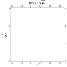
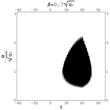
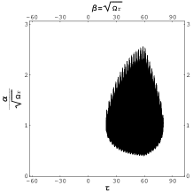
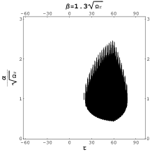
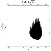
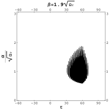
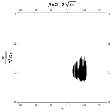
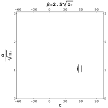
Figure 5: Evolution of $\Sigma$ with each detector initially in a squeezed state with minimum uncertainty. The parameters are the same as those in Fig. 1 (left) except $\alpha$ and $\beta$, which are indicated in the plots. In the dark spots of the above plots, $\Sigma<0$ and the detectors are entangled. One can see that the parameters in $(\alpha,\beta)$ space far away from the ones for the ground state (at $(\alpha,\beta)=(\sqrt{\Omega_{r}},\sqrt{\Omega_{r}})$, in the third plot from the left in the upper row) tend to increase the value of $\Sigma$, namely, decrease the degree of entanglement.

IV.2 Dynamics with Truncated RDM

At early times in the perturbative regime the leakage of amplitudes to higher excited states are negligibly small, so we expect the two detectors can be approximately seen as a two 2-level systems (2LS). For this kind of $2\times 2$ system the two 2LS are entangled if the partial transpose of the RDM $\rho^{R}_{n_{A}n_{B},n^{\prime}_{A}n^{\prime}_{B}}$ in $(\ref{truncRho})$ has a negative eigenvalue, namely if one of the inequalities

$$\rho^{R}_{10,10}\rho^{R}_{01,01}-\rho^{R}_{11,00}\rho^{R}_{00,11}\geq 0,$$ (20)

and

$$\rho^{R}_{00,00}\rho^{R}_{11,11}-\rho^{R}_{10,01}\rho^{R}_{01,10}\geq 0,$$ (21)

is violated. Reznik discovered Reznik03 that the inequality $(\ref{keyineq})$ for the RDM of the two 2LS will always be violated in TDPT with integration domain extended to ${\bf R}^{2}$ (denoted as TDPT_∞; Cf. $(\ref{R1010TDPT})$-$(\ref{R1111TDPT})$), according to which he claimed that quantum entanglement can be generated outside the light cone.

In Appendix B we derive the truncated RDM for two UD detectors explicitly. Comparing this result with the full dynamics, we can make the following observations:

1) Reznik’s conclusion based on TDPT_∞ is not generic for all values of the initial moment $\tau_{0}$, the proper acceleration $a$, the natural frequency $\Omega$, or the coupling strength $\gamma$. Actually, the key result Eq.(18) in Reznik03 is correct only at the moment $\tau=-\tau_{0}$ in the TDPT regime that entanglement creation can occur.

2) Beyond the TDPT_∞ regime, our result shows that once quantum entanglement is created, it only survives in a finite duration. The two detectors are always separable at $\tau<0$ and at late times.

3) The inequality $(\ref{keyineq})$ implies that, if the quantum state of the detectors is separable, then from $(\ref{truncRho})$ one has

$$0\leq{\cal J}^{AA^{\prime}}{\cal J}^{BB^{\prime}}-{\cal J}^{AB}{\cal J}^{A^{\prime}B^{\prime}}={\Sigma\Omega^{2}\det(V+V_{0})\over 16\hbar^{10}\left[\left<\right.Q_{A}^{2}\left.\right>\left<\right.Q_{B}^{2}\left.\right>-\left<\right.Q_{A},Q_{B}\left.\right>^{2}\right]^{2}},$$ (22)

which is a product of the quantity $\Sigma$ and a positive definite function of time. (Here $V_{0}\equiv(\hbar/2){\rm diag}(\Omega^{-1},\Omega,\Omega^{-1},\Omega)$ is the covariance matrix for two free detectors in their ground states.) Thus the criterion of separability $(\ref{keyineq})$, though derived from the RDM of the truncated oscillator, is actually equivalent to $\Sigma\geq 0$, which is the sufficient and necessary criterion for Gaussian states in the full dynamics LH2009 . In other words, the RDM of the two oscillators each with a truncated spectrum, including only up to the first excited state, possesses the complete information pertaining to the separability of the two detectors in Gaussian states.

We illustrate the time evolution of the exact $|\rho^{R}_{11,00}|$ and $|\rho^{R}_{10,10}|$ from $(\ref{truncRho})$ in Fig. 6, where the value of $|\rho^{R}_{11,00}|$ is highly dependent on the behavior of the cross correlators (see Eqs. $(\ref{r1100WCL})$-$(\ref{aBmWCL})$): it grows as the amplitude of the cross correlators grows. At the same time the growing cross correlators tend to decrease the value of $|\rho^{R}_{10,10}|$. Combining these two factors we find, in exactly the same duration that the detectors are entangled in the full dynamics, $|\rho^{R}_{11,00}|$ exceeds $|\rho^{R}_{10,10}|$ and violates the inequality $(\ref{keyineq})$.

Figure 6: Evolution of $|\rho^{R}_{11,00}|$ (dotted curve) and $|\rho^{R}_{10,10}|$ (solid curve) of the truncated RDM under the same condition as in Fig. 2 (left). The duration the detectors are entangled determined by the condition $|\rho^{R}_{11,00}|>|\rho^{R}_{10,10}|$ matches exactly with the result determined by $c_{-}<\hbar/2$.

V Discussion

V.1 Summary of our findings

We have studied the entanglement creation process of two uniformly accelerated UD detectors moving in opposite directions in the Minkowski vacuum of a massless scalar field. The two detectors are causally disconnected during the whole history and are far apart at late times.

For two detectors initially in their ground states, entanglement creation does occur under some specific conditions: if the initial time is negative and not very close to zero, the coupling strength $\gamma$ between each detector and the field is not too large, and the ratio of the proper acceleration $a$ to the natural frequency of the detectors $\Omega$ is at some moderate value. The moment of entanglement creation, if any, is always at positive $\tau$. Once quantum entanglement is created it can last for a lifetime much longer than the natural period of the detectors in some parameter range, while entanglement always disappears in a finite time.

For two detectors each initially in a squeezed state, similar entanglement creation can also occur if the squeeze parameters in the initial state of both detectors are sufficiently small so the initial state is close enough to the direct product of the ground states.

Moreover, we find that the RDM of two oscillators each with a truncated spectrum up to the first excited state contains the complete information about the separability of the oscillators in Gaussian states. In Appendices A and B we see that in TDPT_∞ regime, where the integration domain has been extended to ${\bf R}^{2}$, the growing rates of the matrix elements of the truncated RDM can be estimated well, but one has to be careful in obtaining the ratio of different matrix elements. While TDPT_∞ results are Markovian, we find TDPT still keeps some of the non-Markovian features.

The dependence of entanglement dynamics on the initial state, the fiducial time, and the non-Markovian features shown above are beyond the scope of Massar and Spindel’s steady-state calculation MS06 . In addition, there are some other interesting differences between our findings in (3+1)D UD detector theory and MS’s in (1+1)D U-RSG model. First, in our analysis $\Lambda_{0}$ and $\Lambda_{1}$ corresponding to the ultraviolet cutoffs in (3+1)D UD detector theory explicitly enter the entanglement dynamics, while the infrared cutoff in (1+1)D U-RSG model does not affect the degree of entanglement in MS’s result because they only considered the cases where their constant $K$, which is a product of the coupling strength and the very long duration of the interaction corresponding to the infrared divergence, is always much greater than all other parameters, such that the higher-order terms in the $K$-expansion of the logarithmic negativity can be neglected. Second, while in both cases quantum entanglement between the detectors can be created after the moment in Minkowski time that the distance between the detectors is a minimum, the lifetimes of the created entanglement in our case are usually much longer than the natural period of the detectors, in contrast to the short lifetimes of entanglement in MS’s (1+1)D results. Finally, in our (3+1)D case entanglement creation is totally suppressed in the strong coupling regime and can manifest in the weak coupling limit, while in MS’s result entanglement generation is a non-pertubative phenomena so there is no entanglement creation in their weak coupling regime.

V.2 Quantum nonlocality, causality, and reference frames

Entanglement creation between two causally disconnected objects as we have captured in this work may be viewed as a manifestation of “quantum nonlocality” in quantum physics. Quantum entanglement between two localized objects can be generated by allowing them to interact with a common quantum field even though they do not exchange any classical information. Foremost our results testify to the important fact that quantum nonlocality does not violate causality CK09 . Notice that quantum entanglement can be recognized and put to use (as in QIP) only by those “spectators” who can access the information from both detectors. From the viewpoint of the separate detectors each can never find out the existence of the other from its own RDM, nor the quantum entanglement between them. There is no transmittal of physical information between them and causality (of information) is always respected.

This fact also means that the existence of a“spectator” is essential when we refer to the dynamics of entanglement between the two localized parties outside of causal contact. The spectator is causally connected to (and thus can “see”) both parties and can recognize the quantum entanglement between them through its own observation of both. Recall that in Ref. LCH2008 we found that entanglement dynamics for two quantum objects in relativistic motion depend on the choice of reference frames or coordinates (Minkowski or Rindler, for example). One may debate on which coordinate is “better” or more “objective” for the depiction of entanglement dynamics. Our results show that the only physically meaningful one in a given physical setup for describing the entanglement dynamics of the system is that of the spectator. This is of course not unique, but there are well-established ways to relate what is measured by one spectator to another with considerations of time-slicing (see, e.g., LCH2008 ) and transformation laws of reference frames in relativity theory.

V.3 Quantum entanglement generated by collision

The setup of our problem can also mimic the situation of two ions of the same charge in a head-on collision. Quantum entanglement is generated in the later stage of the collision when the two ions are moving apart, once the trajectories of the ions possess the right kind of symmetry to enhance the field correlations as those in the present problem (see Appendix A.2). There is no energy exchange between the two ions during the entanglement creation process of this kind.

It has been shown that two atoms coupled with a common field vacuum in a cavity can get entangled in a “collision” ZG00 ; Haro01 . These entangling processes could be interpreted as a consequence of virtual quanta exchange in a van der Waal potential, analogous to those with the coulomb interaction in electron-electron scattering. In Haro01 the interaction time is much longer than the propagation time of photons across the spatial separation between the atoms, and energy exchange between two atoms is clearly present. These cases where entanglement generation occurring well inside the light cone is different from the present setup but closer to the situation we considered in LH2009 , where quantum entanglement is established mainly by retarded mutual influences.

Note that particle (or atom, molecule) collisions in non-relativistic classical and quantum mechanics are usually described by an effective Hamiltonian with a direct, nonlocal, inter-particle interaction (e.g. a potential $V(|{\bf r}_{1}-{\bf r}_{2}|)$, where ${\bf r}_{1,2}$ are the positions of the particles). Direct interaction always generates correlation between the particles, classical or quantum. The nonlocality of the interaction, on the other hand, is a consequence of coarse graining from a more fundamental local theory, resulting in an effective theory description. The particles in this non-relativistic regime cannot resolve the time scale for information propagating back and forth between them. Thus the generation of correlation by this kind of nonlocal direct interaction happens in a time scale during which two particles have causal contact for a long time. One cannot tell whether correlations can be created between two causally disconnected particles in this kind of effective theories. Moreover, with this kind of nonlocal direct interaction, if one does not further introduce a spatial range of interaction associated with a coarse-graining in time, even classical correlation will be nonlocal and cannot be described by any local hidden-variable theory.

Acknowledgment SYL wishes to thank Daniel Braun for illuminating discussions during his visit to the Joint Quantum Institute, University of Maryland and National Institute of Standards and Technology, where this work was first motivated and commenced. BLH wishes to thank the hospitality of National Center for Theoretical Sciences and the QIS group at National Cheng Kung University of Taiwan. This work is supported partially by grants from LPS, NSF grants PHY-0426696, PHY-0801368 and DARPA-HR0011-09-1-0008.

Appendix A Matrix elements in time-dependent perturbation theory

In TDPT, one expands the wave function of the two detectors in terms of the energy eigenstates $\varphi_{m}(Q_{A})$ and $\varphi_{n}(Q_{B})$ of the free detectors as

$$\psi(\tau)=\sum_{m^{\prime},n^{\prime}}C_{m^{\prime}n^{\prime},mn}e^{-i(\omega_{m^{\prime}}+\omega_{n^{\prime}})\tau-i(\omega_{m}+\omega_{n})\tau_{0}}\varphi_{m^{\prime}}(Q_{A})\varphi_{n^{\prime}}(Q_{B}),$$ (23)

then calculates the first few factors in the perturbative series of $C_{m^{\prime}n^{\prime},mn}$ assuming a small coupling constant $\lambda_{0}$, namely, $C_{m^{\prime}n^{\prime},mn}\equiv\sum_{N}\lambda_{0}^{N}C_{m^{\prime}n^{\prime},mn}^{(N)}$. Here $\omega_{n}\equiv E_{n}/\hbar=\Omega[n+(1/2)]$. For the initial state $(\ref{initGauss})$, to lowest order in $\lambda_{0}$, the elements of the RDM of the detectors are

$$\rho^{R}_{10,10} \approx {\lambda_{0}^{2}\over 2\hbar\Omega}\int_{\tau_{0}}^{\tau}ds\int_{\tau_{0}}^{\tau}ds^{\prime}e^{-i\Omega(s-s^{\prime})}D^{+}\left(z^{\mu}_{A}(s),z^{\nu}_{A}(s^{\prime})\right),$$ (24)

$$\rho^{R}_{10,01} \approx {\lambda_{0}^{2}\over 2\hbar\Omega}\int_{\tau_{0}}^{\tau}ds\int_{\tau_{0}}^{\tau}ds^{\prime}e^{-i\Omega(s-s^{\prime})}D^{+}\left(z^{\mu}_{A}(s),z^{\nu}_{B}(s^{\prime})\right),$$ (25)

$$\rho^{R}_{11,00} \approx -{\lambda_{0}^{2}e^{-2i\Omega\tau}\over 2\hbar\Omega}\int_{\tau_{0}}^{\tau}ds\int_{\tau_{0}}^{\tau}ds^{\prime}e^{i\Omega(s+s^{\prime})}D^{+}\left(z^{\mu}_{A}(s),z^{\nu}_{B}(s^{\prime})\right),$$ (26)

$$\rho^{R}_{11,11} \approx \left({\lambda_{0}^{2}\over 2\hbar\Omega}\right)^{2}\int_{\tau_{0}}^{\tau}dsds^{\prime}d\bar{s}d\bar{s}^{\prime}e^{i\Omega(s+s^{\prime}-\bar{s}-\bar{s}^{\prime})}\left[D^{+}\left(z^{\rho}_{A}(\bar{s}),z^{\sigma}_{B}(\bar{s}^{\prime})\right)D^{+}\left(z^{\mu}_{A}(s),z^{\nu}_{B}(s^{\prime})\right)+\right.$$ (27)

$$\left.D^{+}\left(z^{\rho}_{A}(\bar{s}),z^{\mu}_{A}(s)\right)D^{+}\left(z^{\sigma}_{B}(\bar{s}^{\prime}),z^{\nu}_{B}(s^{\prime})\right)+D^{+}\left(z^{\rho}_{A}(\bar{s}),z^{\nu}_{B}(s^{\prime})\right)D^{+}\left(z^{\sigma}_{B}(\bar{s}^{\prime}),z^{\mu}_{A}(s)\right)\right],$$

etc., where $D^{+}$ is the positive frequency Wightman function of the massless scalar field in Minkowski vacuum, given by

$$D^{+}(z_{j}^{\mu},z_{j^{\prime}}^{\nu}) \equiv \left<\right.0_{M}\left.\right|\phi\left(z^{\mu}_{j}\right)\phi\left(z^{\nu}_{j^{\prime}}\right)\left|\right.0_{M}\left.\right>$$ (28)

$$= \int{\hbar d^{3}k\over(2\pi)^{3}2\omega}e^{-\omega\epsilon}e^{-i\omega(z_{j}^{0}-z_{j^{\prime}}^{0})+i{\bf k}\cdot({\bf z}_{j}-{\bf z}_{j^{\prime}})}$$

$$= {\hbar/4\pi^{2}\over\left|{\bf z}_{j}-{\bf z}_{j^{\prime}}\right|^{2}-\left(z_{j}^{0}-z_{j^{\prime}}^{0}-i\epsilon\right)^{2}}$$

with $j,j^{\prime}=A,B$ and the frequency $\omega\equiv|{\bf k}|$ for the massless scalar field. $\epsilon$ is a small positive real number serving as a regulator at high frequency in ${\bf k}$-integration.

A.1 The regulators

In obtaining $\rho^{R}_{1010}$ in $(\ref{R1010TDPT})$, one could insert the trajectory of the detector A into $(\ref{wightgen})$, which gives the Wightman function as

$$D^{+}(z_{A}^{\mu}(s),z_{A}^{\nu}(s^{\prime}))={\hbar/4\pi^{2}\over-{4\over a^{2}}\sinh{a\over 2}\Delta\left(\sinh{a\over 2}\Delta-i\epsilon a\cosh aT\right)+\epsilon^{2}},$$ (29)

with $T\equiv(s+s^{\prime})/2$ and $\Delta\equiv s-s^{\prime}$. Conventional wisdom says that the value of $\epsilon$ is extremely small, so the expression of the Wightman function could be replaced by BD82

$$D^{\prime+}(z_{A}^{\mu}(s),z_{A}^{\nu}(s^{\prime}))={\hbar/4\pi^{2}\over-{4\over a^{2}}\sinh^{2}{a\over 2}(\Delta-i\epsilon^{\prime})}$$ (30)

$$\approx {\hbar/4\pi^{2}\over-{4\over a^{2}}\sinh{a\over 2}\Delta\left(\sinh{a\over 2}\Delta-i\epsilon^{\prime}a\cosh{a\over 2}\Delta\right)+\epsilon^{\prime 2}\cosh a\Delta},$$

which is independent of $T$. Indeed, when $aT$ is small, the original $D^{+}$ and the modified $D^{\prime+}$ have similar positions of poles and similar behavior around the poles in the complex $\Delta$ plane.

However, as shown in Fig. 7, only the modified $D^{\prime+}$ will give a linear-growing phase in transient like

$$\rho_{10,10}^{R\infty}=2\gamma\eta/(e^{2\pi\Omega/a}-1),$$ (31)

where the growing rate $\rho_{10,10}^{R\infty}/\eta$ can be obtained by extending the integration domain of $(s,s^{\prime})$ to ${\bf R}^{2}$, namely, from TDPT_∞. In contrast, the original $D^{+}$ leads to a totally different behavior of $\rho_{10,10}^{R}$: It is linearly decreasing in the beginning and saturates after $\tau>-a^{-1}\ln\epsilon$.

Learning from what we did in taking the coincidence limit of the self correlators LH2006 , we find that, if we put the small shifts $\epsilon_{0}$ and $\epsilon_{1}$ at the upper and lower bounds of the $s$ and $s^{\prime}$ integration domain, such as

$$\rho^{R}_{10,10}\approx{\lambda_{0}^{2}\over 2\hbar\Omega}\int_{\tau_{0}}^{\tau+\epsilon_{1}}ds\int_{\tau_{0}+\epsilon_{0}}^{\tau}ds^{\prime}e^{-i\Omega(s-s^{\prime})}D^{+}\left(z^{\mu}_{A}(s),z^{\nu}_{A}(s^{\prime})\right),$$ (32)

and take the $\epsilon$ in $D^{+}$ to zero limit, then the exotic behavior of $D^{+}$ will be altered and we recover the results obtained by using the modified $D^{\prime+}$ with $\epsilon^{\prime}$ corresponding to $\epsilon_{0}$ when $\epsilon_{0}=\epsilon_{1}$. So we interpret $\epsilon$ as the mathematical cutoff, which should be taken the zero limit at some point of calculation, while the $\epsilon_{0}$, $\epsilon_{1}$ in $(\ref{R1010phys})$ and the $\epsilon^{\prime}$ in $(\ref{modifiedDp})$ are physical cutoffs corresponding to the time resolution of the detectors and related to the constants $\Lambda_{0}$ and $\Lambda_{1}$ in the expressions for the self correlators LH2006 . The replacement from $(\ref{originalDp})$ to $(\ref{modifiedDp})$ actually changes the interpretation of the regulator.

Figure 7: Early-time evolutions of the $\rho_{10,10}^{R}$ in TDPT with the original positive frequency Wightman function, $D^{+}(z_{A}^{\mu}(s),z_{A}^{\nu}(s^{\prime}))$ in Eq. $(\ref{originalDp})$ (dashed curve) with $\epsilon=e^{-14-\gamma_{e}}/\Omega$ ($\gamma_{e}$ is the Euler’s constant), the $\rho_{10,10}^{R}$ with the modified one, $D^{\prime+}(z_{A}^{\mu}(s),z_{A}^{\nu}(s^{\prime}))$ in Eq. $(\ref{modifiedDp})$ (solid curve) with $\epsilon^{\prime}=e^{-14-\gamma_{e}}/\Omega$, and the $\rho_{10,10}^{R}$ in $(\ref{R1010phys})$ with the original $D^{+}(z_{A}^{\mu}(s),z_{A}^{\nu}(s^{\prime}))$ and $\epsilon=e^{-30}/\Omega$, together with the physical cutoffs $\epsilon_{0}=\epsilon_{1}=e^{-14-\gamma_{e}}/\Omega\gg\epsilon$ (dots). The left and the right plots are the same results but shown in different scales to stress that the early-time behavior of the dotted curve really matches with the climbing solid curve. Here $\gamma=10^{-5}$ and $\Omega=2.3$. The slope of the dotted curve in its linear growing phase agrees quite well with $2\gamma/(e^{2\pi\Omega/a}-1)$ in $(\ref{R1010PTinf})$.

A.2 Calculating $|\rho^{R}_{11,00}|$

Usually in obtaining $\rho^{R}_{10,10}$, TDPT is good from $\eta\equiv\tau-\tau_{0}\gg\Lambda_{1}/\Omega$ up to $\eta\sim O(1/\gamma)$ LH2006 with $\gamma\equiv\lambda_{0}^{2}/8\pi$ (here the masses of both harmonic oscillators in the detectors have been set to $m_{0}=1$ and the proper accelerations of the detectors are not extremely large). This is a large duration if $\gamma$ is small, which is consistent with the assumption of TDPT, so it is commonly argued that extending the domain of $s$ integration from $(\tau_{0},\tau)$ to $(-\infty,\infty)$ in this duration would not change the results too much, that is, the TDPT_∞ results should be very close to the TDPT results.

In Ref.Reznik03 , Reznik compared the absolute values of $|\rho^{R}_{11,00}|$ and $|\rho^{R}_{10,10}|$ in TDPT_∞ and discovered that the former is always greater than the latter, then drew the conclusion that the two detectors are always entangled. Nevertheless, with the extended integration domain, both $|\rho^{R}_{11,00}|$ and $|\rho^{R}_{10,10}|$ are infinities, which are meaningless as elements of any density matrix. Usually one divides $|\rho^{R}_{10,10}|$ by the infinite duration of interaction and interprets the result as the transition probability per unit time in the linear-growing phase in TDPT regime BD82 . But the choice of proper duration for $|\rho^{R}_{11,00}|$ and the interpretation for the result could be tricky (see Appendix B for more details). Further, our numerical results show that if we calculate $|\rho^{R}_{11,00}|$ with a finite integration domain and a nonzero regulator $\epsilon$, the value of $(\ref{R1100TDPT})$ after integration can be quite different from those obtained in Ref.Reznik03 .

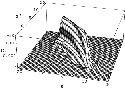
Figure 8: (Left) An example of $|D^{+}(z_{A}^{\mu}(s),z_{B}^{\nu}(s^{\prime}))|$ in Eq. $(\ref{DpAB})$. Here $\epsilon=e^{-8}$ and $a=1$. One can see that the correlation of the massless scalar field at $z_{A}^{\mu}(s)$ and $z_{B}^{\nu}(s^{\prime})$ is enhanced around $s^{\prime}=-s$. Such an enhancement will be suppressed if the trajectories of the detectors are off the $z_{A}^{\mu}(s)$ and $z_{B}^{\nu}(s^{\prime})$ in this paper or the scalar field is massive. (Right) Contour plot of the same $|D^{+}(z_{A}^{\mu}(s),z_{B}^{\nu}(s^{\prime}))|$. The long-dashed lines, solid lines, short-dashed lines, and dotted lines are borders of the integration domain at $\tau=-10$, $0$, $1/a\sinh^{-1}\epsilon^{-1}(\approx 8.69)$, and $15$, respectively.

To calculate $\rho^{R}_{11,00}$, one substitutes the trajectories $z_{A}^{\mu}$ and $z_{B}^{\mu}$ into the positive frequency Wightman function and obtain

$$D^{+}(z_{A}^{\mu}(s),z_{B}^{\nu}(s^{\prime}))={\hbar/4\pi^{2}\over{4\over a^{2}}\cosh aT\left(\cosh aT+i\epsilon a\sinh{a\over 2}\Delta\right)+\epsilon^{2}}.$$ (33)

Now $D^{+}(z_{A}^{\mu}(s),z_{B}^{\nu}(s^{\prime}))$ is regular everywhere in $(s,s^{\prime})$ plane. For small finite $\epsilon$, since $\cosh aT\geq 1$, the $\epsilon^{2}$ term in the denominator can always be neglected, but the $\epsilon$ term cannot. If $\epsilon\sinh a\Delta/2\ll\cosh aT$, then $D^{+}\approx a^{2}/16\pi^{2}\cosh^{2}aT$, which is a function of $T$ only and peaks around $T=0$. For $\Delta$ sufficiently large such that $\epsilon a\sinh a\Delta/2\gtrsim 1$, however, $|D^{+}|$ will be suppressed. So $|D^{+}(z_{A}^{\mu}(s),z_{B}^{\nu}(s^{\prime}))|$ looks like a ridge at $T\approx 0$ and spread with the width $4\tau_{1}$ in $\Delta$ direction, where $\tau_{1}\equiv(1/a)\sinh^{-1}(1/a\epsilon)\approx(1/a)\ln(2/a\epsilon)$ (see Fig. 8).

Suppose the coupling is switched on at the initial moment $\tau_{0}<0$. From the landscape of $D^{+}(z_{A}^{\mu}(s),z_{B}^{\nu}(s^{\prime}))$ shown in Fig. 8, the evolution of $|\rho^{R}_{11,00}|$ will have three stages:

(i) When $\tau_{0}<\tau<0$, $D^{+}(z_{A}^{\mu}(s),z_{B}^{\nu}(s^{\prime}))$ is small all over the ${\bf s}$-integration domain (within the square with two sides in long-dashed lines in Fig. 8 (right)), so the change in $|\rho^{R}_{11,00}|$ is tiny.

(ii) At about $\tau=0$, the edge of the ${\bf s}$-integration domain [within the square with all sides in solid lines in Fig. 8 (right)] touches the ridge of $|D^{+}(z_{A}^{\mu}(s),z_{B}^{\nu}(s^{\prime}))|$ around $T=0$, which gives obvious contribution to the result. As $\tau$ grows, more and more portion of the ridge are included in the integration domain. Since the height of the ridge is almost constant in the $\Delta$ direction, $|\rho^{R}_{11,00}|$ grows linearly in $\tau$.

(iii) The linear growth terminates at about $\tau=\tau_{1}$. Then the integration domain has covered almost all the ridge so that $|D^{+}(z_{A}^{\mu}(s),z_{B}^{\nu}(s^{\prime}))|$ does not add obvious contribution after $\tau=\tau_{1}$ and $|\rho^{R}_{11,00}|$ saturates at some constant.

From the argument in Sec. A.1, one should take $\epsilon\to 0$ so $\tau_{1}$ and the width of the ridge in the $\Delta$ direction is virtually infinite. Then stage (ii) will be terminated around $\tau\approx|\tau_{0}|$ because only a portion of the ridge with $|\Delta|\lesssim 2|\tau_{0}|$ is covered in the integration domain. This could be enough to make the value of $|\rho^{R}_{11,00}|$ exceeds $|\rho^{R}_{10,10}|$ and the two detectors get entangled, if $|\tau_{0}|$ is sufficiently large. On the other hand, for $\tau_{0}\geq 0$, the linear growth of stage (ii) never occurs, and $|\rho^{R}_{11,00}|$ is always less than $|\rho^{R}_{10,10}|$.

Thus one can see that the value of $|\rho^{R}_{11,00}|$ as well as the ratio $|\rho^{R}_{11,00}|/|\rho^{R}_{10,10}|$ have complicated evolution in time even in TDPT. Their behaviors are quite different from the constant ones obtained in Ref.Reznik03 .

Appendix B Truncated reduced density matrix of the two detectors

Generalize the method applied in LH2006 for one single detector, the elements of the RDM in eigen-energy representation can be read off by comparing the coefficients of the $s_{j}^{n_{j}}$ terms in both sides of the following equation,

$$\sum_{n_{i}=0}^{\infty}\left[\rho^{R}_{n_{A}n_{A^{\prime}},n_{B}n_{B^{\prime}}}\prod_{j}s_{j}^{n_{j}}\sqrt{{2^{n_{j}}\over n_{j}!}}\right]=\sqrt{\prod_{j}K_{j}\over{\cal G}\det\tilde{G}}\,\exp\sum_{i,j}s_{i}\left[K_{i}(\tilde{G}^{-1})^{ij}K_{j}-\delta^{ij}\right]s_{j},$$ (34)

where $i,j=A,A^{\prime},B,B^{\prime}$, $K_{A}=K_{A^{\prime}}=K_{B}=K_{B^{\prime}}=K\equiv\sqrt{\Omega_{r}/\hbar}$, ${\cal G}$ is defined by

$${\cal G}\equiv 4\left[\left<\right.Q_{A}^{2}\left.\right>\left<\right.Q_{B}^{2}\left.\right>-\left<\right.Q_{A},Q_{B}\left.\right>^{2}\right],$$ (35)

and $\tilde{G}$ is parametrized in

$$\tilde{G}\equiv\left(\begin{array}[]{cccc}a_{A+}+ib_{A}+{K_{A}^{2}\over 2}&a_{A-}&a_{X+}+ib_{X+}&a_{X-}+ib_{X-}\\ a_{A-}&a_{A+}-ib_{A}+{K_{A^{\prime}}^{2}\over 2}&a_{X-}-ib_{X-}&a_{X+}-ib_{X+}\\ a_{X+}+ib_{X+}&a_{X-}-ib_{X-}&a_{B+}+ib_{B}+{K_{B}^{2}\over 2}&a_{B-}\\ a_{X-}+ib_{X-}&a_{X+}-ib_{X+}&a_{B-}&a_{B+}-ib_{B}+{K_{B^{\prime}}^{2}\over 2}\end{array}\right),$$ (36)

with the factors

$$a_{A\pm} = {1\over 2{\cal G}}\left[V^{11}\pm{4\over\hbar^{2}}\left(V^{-1}\right)^{22}\det V\right],$$ (37)

$$a_{B\pm} = {1\over 2{\cal G}}\left[V^{33}\pm{4\over\hbar^{2}}\left(V^{-1}\right)^{44}\det V\right],$$ (38)

$$a_{X\pm} = -{1\over 2{\cal G}}\left[V^{13}\pm{4\over\hbar^{2}}\left(V^{-1}\right)^{24}\det V\right],$$ (39)

$$b_{A} = {2\over\hbar{\cal G}}\left(\left<\right.P_{A},Q_{B}\left.\right>\left<\right.Q_{A},Q_{B}\left.\right>-\left<\right.P_{A},Q_{A}\left.\right>\left<\right.Q_{B}^{2}\left.\right>\right),$$ (40)

$$b_{B} = {2\over\hbar{\cal G}}\left(\left<\right.P_{B},Q_{A}\left.\right>\left<\right.Q_{A},Q_{B}\left.\right>-\left<\right.P_{B},Q_{B}\left.\right>\left<\right.Q_{A}^{2}\left.\right>\right),$$ (41)

$$b_{X\pm} = {1\over\hbar{\cal G}}\left[\left(\left<\right.P_{A},Q_{A}\left.\right>\left<\right.Q_{A},Q_{B}\left.\right>-\left<\right.P_{A},Q_{B}\left.\right>\left<\right.Q_{A}^{2}\left.\right>\right)\pm\right.$$ (42)

$$\,\,\,\left.\left(\left<\right.P_{B},Q_{B}\left.\right>\left<\right.Q_{A},Q_{B}\left.\right>-\left<\right.P_{B},Q_{A}\left.\right>\left<\right.Q_{B}^{2}\left.\right>\right)\right].$$

These $a$ and $b$ factors are obtained by solving the coefficients $G^{ij}$ in the Gaussian RDM of the detectors $\rho^{R}\sim\exp-\sum_{i,j}Q_{i}G^{ij}Q_{j}$ in terms of the two-point correlators. Here $V^{ij}$ are the elements of the covariance matrix

$$V=\left(\begin{array}[]{cc}{\bf v}_{AA}&{\bf v}_{AB}\\ {\bf v}_{BA}&{\bf v}_{BB}\end{array}\right),$$ (43)

in which the elements of the $2\times 2$ matrices ${\bf v}_{ij}$ are symmetrized two-point correlators ${\bf v}_{mn}{}^{\mu\nu}=\left<\right.{\cal R}^{\mu}_{m},{\cal R}^{\nu}_{n}\left.\right>\equiv\left<\right.({\cal R}^{\mu}_{m}{\cal R}^{\nu}_{n}+{\cal R}^{\nu}_{n}{\cal R}^{\mu}_{m})\left.\right>/2$ with ${\cal R}^{\mu}_{m}=(Q_{m}(t),P_{m}(t))$, $\mu,\nu=1,2$ and $m,n=A,B$.

Up to the first excited states of both detectors, the truncated RDM of the two detectors in eigen-energy representation reads

$$\rho^{R}_{n_{A}n_{B},n^{\prime}_{A}n^{\prime}_{B}}\approx\left(\begin{array}[]{cccc}g&0&0&gK^{2}{\cal J}^{A^{\prime}B^{\prime}}\\ 0&gK^{2}{\cal J}^{BB^{\prime}}&gK^{2}{\cal J}^{A^{\prime}B}&0\\ 0&gK^{2}{\cal J}^{AB^{\prime}}&gK^{2}{\cal J}^{AA^{\prime}}&0\\ gK^{2}{\cal J}^{AB}&0&0&gK^{4}\left[{\cal J}^{AB}{\cal J}^{A^{\prime}B^{\prime}}+{\cal J}^{AA^{\prime}}{\cal J}^{BB^{\prime}}+{\cal J}^{AB^{\prime}}{\cal J}^{A^{\prime}B}\right]\end{array}\right)$$ (44)

with $n_{A},n_{B},n^{\prime}_{A},n^{\prime}_{B}=0,1$, ${\cal J}\equiv\tilde{G}^{-1}$, and

$$g\equiv{\Omega/\hbar\over\sqrt{{\cal G}\det\tilde{G}}}.$$ (45)

Here we use the basis $(n_{A},n_{B})=\{00,01,10,11\}$ for $\rho^{R}$.

What TDPT_∞ could describe well is the transient behavior during $\Omega^{-1}\ll\tau<|\tau_{0}|\ll 1/2\gamma$ while $\Omega^{-1}\ll\tau-\tau_{0}\ll 1/\gamma$ with $\tau_{0}<0$, when the amplitudes of the oscillating cross correlators are linearly increasing, while the magnitudes of the self correlators are still in transient and growing linearly, too. In this regime, $\left<\right.Q_{A},Q_{B}\left.\right>$ can be approximated by $(\ref{t0ggt})$, which also yields

$$\left<\right.P_{A},Q_{B}\left.\right>\approx\left<\right.Q_{A},P_{B}\left.\right>\approx{\hbar\gamma\over\Omega\sinh{\pi\Omega\over a}}\left[2\Omega\tau\sin 2\Omega\tau+\left({\pi\Omega\over a}\coth{\pi\Omega\over a}-1\right)\cos 2\Omega\tau\right],$$ (46)

$$\left<\right.P_{A},P_{B}\left.\right>\approx{\hbar\gamma\over\sinh{\pi\Omega\over a}}\left[2\Omega\tau\cos 2\Omega\tau-\left({\pi\Omega\over a}\coth{\pi\Omega\over a}-1\right)\sin 2\Omega\tau\right],$$ (47)

up to $O(\gamma)$. Together with the $O(\gamma)$ results of the self correlators in TDPT regime from LH2006 with $m_{0}=1$,

$$\left<\right.Q_{A}^{2}\left.\right>=\left<\right.Q_{B}^{2}\left.\right> \approx {\hbar\over 2\Omega}+$$ (48)

$${\hbar\gamma\over\Omega}\left[\left(\coth{\pi\Omega\over a}-1\right)\eta+{2\over\pi\Omega}(\Lambda_{0}-\ln a)\sin^{2}\Omega\eta+{\sin 2\Omega\eta\over 2\Omega}\right],$$

$$\left<\right.Q_{A},P_{A}\left.\right>=\left<\right.Q_{B},P_{B}\left.\right> \approx {\hbar\gamma\over 2\Omega}\left[\left(\coth{\pi\Omega\over a}-1\right)+{2\over\pi}(\Lambda_{0}-\ln a)\sin 2\Omega\eta+\cos 2\Omega\eta\right],$$ (49)

$$\left<\right.P_{A}^{2}\left.\right>=\left<\right.P_{B}^{2}\left.\right> \approx {\hbar\Omega\over 2}+$$ (50)

$${\hbar\gamma\Omega}\left[\left(\coth{\pi\Omega\over a}-1\right)\eta+{2\over\pi\Omega}\left[\Lambda_{1}-\ln a+(\Lambda_{0}-\ln a)\cos^{2}\Omega\eta\right]-{\sin 2\Omega\eta\over 2\Omega}\right],$$

one finds that, for the detectors initially in their ground states,

$$a_{A+}=a_{B+} \approx {\Omega\over 2\hbar}+{\gamma\over\hbar}\left[{1\over\pi}\left[\Lambda_{1}-\ln a+(\Lambda_{0}-\ln a)\cos 2\Omega\eta\right]-{1\over 2}\sin 2\Omega\eta\right],$$ (51)

$$a_{A-}=a_{B-} \approx {\gamma\over\hbar}\left[{2\Omega\eta\over e^{2\pi\Omega/a}-1}+{1\over\pi}(\Lambda_{0}+\Lambda_{1}-2\ln a)\right],$$ (52)

$$a_{X+} \approx {\gamma\over\hbar\sinh{\pi\Omega\over a}}\left[2\Omega\tau\cos 2\Omega\tau+\left(1-{\pi\Omega\over a}\coth{\pi\Omega\over a}\right)\sin 2\Omega\tau\right],$$ (53)

$$b_{X+} \approx {\gamma\over\hbar\sinh{\pi\Omega\over a}}\left[-2\Omega\tau\sin 2\Omega\tau+\left(1-{\pi\Omega\over a}\coth{\pi\Omega\over a}\right)\cos 2\Omega\tau\right],$$ (54)

up to $O(\gamma)$, so that

$$\rho^{R}_{11,00} \approx -gK^{2}{a_{X+}-ib_{X+}\over\left({K^{2}\over 2}+a_{A+}\right)^{2}},$$ (55)

$$\rho^{R}_{01,01} \approx -gK^{2}{a_{B-}\over\left({K^{2}\over 2}+a_{A+}\right)^{2}}.$$ (56)

Now the growing rates of $|\rho^{R}_{11,00}|$ and $|\rho^{R}_{01,01}|$ at large $\tau$ agree well with those estimated by TDPT_∞, where both $\eta$ and $\tau$ are replaced by infinities.

Nevertheless, one has to be careful in calculating the ratio of different matrix elements in TDPT_∞. Indeed, at $\Omega\tau\gg\Lambda_{0}$, $\Lambda_{1}$, $|\rho^{R}_{01,01}|$ is approximately proportional to $\eta=\tau-\tau_{0}$ while $|\rho^{R}_{11,00}|$ is approximately proportional to $\tau$, so that $|\rho^{R}_{11,00}|/|\rho^{R}_{10,10}|\approx e^{\pi\Omega/a}\times 2\tau/\eta$, where $\tau$ and $\eta$ do not simply cancel each other. $|\rho^{R}_{11,00}|/|\rho^{R}_{10,10}|$ is actually time-varying, and Eq.(18) in Reznik03 is correct only at the moment $\eta=2\tau$, or $\tau=-\tau_{0}$, which is almost at the end of the TDPT_∞ regime.

Note that, in weak coupling limit,

$$a_{X+} \approx -{\left<\right.Q_{A},Q_{B}\left.\right>\over 8\left<\right.Q_{A}^{2}\left.\right>\left<\right.Q_{B}^{2}\left.\right>}+{1\over 2\hbar^{2}}\left<\right.P_{A},P_{B}\left.\right>,$$ (57)

$$b_{X+} \approx -{1\over 4\hbar}\left[{\left<\right.P_{A},Q_{B}\left.\right>\over\left<\right.Q_{B}^{2}\left.\right>}+{\left<\right.Q_{A},P_{B}\left.\right>\over\left<\right.Q_{A}^{2}\left.\right>}\right],$$ (58)

$$a_{B-} \approx {1\over 8\left<\right.Q_{B}^{2}\left.\right>}-{1\over 2\hbar^{2}}\left<\right.P_{B}^{2}\left.\right>,$$ (59)

so the behavior of $\rho^{R}_{11,00}$ in $(\ref{r1100WCL})$ is highly dependent on the behavior of the cross correlators, while $\rho^{R}_{01,01}$ in $(\ref{r0101WCL})$ is not.

Note also that $(\ref{truncRho})$ in ultraweak coupling limit is numerically consistent with the TDPT results in Appendix A in the time interval $\Omega^{-1}\ll\tau-\tau_{0}\ll 1/\gamma$ for $0<-\tau_{0}\ll 1/2\gamma$. Here $\tau$ can be negative or greater than $|\tau_{0}|$. From the three-stage behavior of the $|\rho^{R}_{11,00}|$ in Appendix A, which depends on the fiducial time $\tau_{0}$, one can see that TDPT still keeps some of the non-Markovian features, though the damping behavior ($\sim e^{-2\gamma\tau}$) has been lost in the coupling constant expansion (cf. the integrands of $(\ref{R1010TDPT})$-$(\ref{R1100TDPT})$ with $(\ref{QXdef})$). On the other hand, the validity range of TDPT_∞ is more restricted. TDPT_∞ is valid only when both $|\rho^{R}_{11,00}|$ and $|\rho^{R}_{11,00}|$ are linearly growing, namely, only in the section $\Omega^{-1}\ll\tau<|\tau_{0}|\ll 1/2\gamma$ of the time interval $\Omega^{-1}\ll\tau-\tau_{0}\ll 1/\gamma$ for TDPT. TDPT_∞ results are Markovian because even the memory of the initial moment is lost after the integration domain is extended.

References

- (1) E. Schrodinger, Proc. Camb. Phil. Soc. 31, 555 (1935).
- (2) A. Einstein, B. Podolsky and N. Rosen, Phys. Rev. 47, 777 (1935).
- (3) S.-Y. Lin, C.-H. Chou and B. L. Hu, Phys. Rev. D 78, 125025 (2008).
- (4) S.-Y. Lin and B. L. Hu, Phys. Rev. D 79, 085020 (2009).
- (5) B. Reznik, Found. Phys. 33, 167 (2003).
- (6) B. Reznik, A. Retzker and J. Silman, Phys. Rev. A 71, 042104 (2005).
- (7) S. Massar and P. Spindel, Phys. Rev. D 74, 085031 (2006).
- (8) J. D. Franson, J. Mod. Opt. 55, 2117 (2008).
- (9) D. Braun, Phys. Rev. A 72, 062324 (2005).
- (10) D. J. Raine, D. W. Sciama, and P. G. Grove, Proc. R. Soc. A 435, 205 (1991).
- (11) S.-Y. Lin and B. L. Hu, Phys. Rev. D. 76, 064008 (2007).
- (12) S.-Y. Lin and B. L. Hu, Class. Quantum Grav. 25, 154004 (2008).
- (13) M. Cliche and A. Kempf, Phys. Rev. A 81, 012330 (2010).
- (14) S.-B. Zheng and G.-C. Guo, Phys. Rev. Lett. 85, 2392 (2000).
- (15) S. Osnaghi, P. Bertet, A. Auffeves, P. Maioli, M. Brune, J. M. Raimond, and S. Haroche, Phys. Rev. Lett. 87, 037902 (2001).
- (16) N. D. Birrell and P. C. W. Davies, Quantum Fields in Curved Space (Cambridge University Press, Cambridge, 1982).