Chaotic Transport and Chronology of Complex Asteroid Families

Abstract

We present a transport model that describes the orbital diffusion of asteroids in chaotic regions of the 3-D space of proper elements. Our goal is to use a simple random-walk model to study the evolution and derive accurate age estimates for dynamically complex asteroid families. To this purpose, we first compute local diffusion coefficients, which characterize chaotic diffusion in proper eccentricity ($e_{p}$) and inclination ($I_{p}$), in a selected phase-space region. Then, a Monte-Carlo-type code is constructed and used to track the evolution of random walkers (i.e. asteroids), by coupling diffusion in ($e_{p}$,$I_{p}$) with a drift in proper semi-major axis ($a_{p}$) induced by the Yarkovsky/YORP thermal effects. We validate our model by applying it to the family of (490) Veritas, for which we recover previous estimates of its age ($\sim 8.3$ Myr). Moreover, we show that the spreading of chaotic family members in proper elements space is well reproduced in our randomk-walk simulations. Finally, we apply our model to the family of (3556) Lixiaohua, which is much older than Veritas and thus much more affected by thermal forces. We find the age of the Lixiaohua family to be $155\pm 36$ Myr.

1 Introduction

As first noted by Hirayama (1918), asteroids can form prominent groupings in the space of orbital elements. These groups, nowadays well-known as asteroid families, are believed to have resulted from catastrophic collisions among asteroids, which lead to the ejection of fragments into nearby heliocentric orbits, with relative velocities much lower than their orbital speeds. To date, several tens of families have been discovered across the whole asteroid Main Belt (e.g. Bendjoya & Zappalà, 2002; Nesvorný et al., 2006). Also, families have been identified among the Trojans (Milani, 1993; Beaugé & Roig, 2001), and most recently, proposed to exist in the Transneptunian region (Brown et al., 2007). Studies of asteroid families are very important for planetary science. Families can be used, e.g. to understand the collisional history of the asteroid Main Belt (Bottke et al., 2005), the outcomes of disruption events over a size range inaccessible to laboratory experiments (e.g. Michel et al., 2003; Durda et al., 2007), to understand the mineralogical structure of their parent bodies (e.g. Cellino et al., 2002) and the effects of related dust “showers” on the Earth (Farley et al., 2006). Obtaining the relevant information is, however, not easy. One of the main complications arises from the fact that the age of a family is, in general, unknown. Thus, accurate dating of asteroid families is an important issue in the asteroid science.

A number of age-determination methods have been proposed so far. Probably the most accurate procedure, particularly suited for young families (i.e. age $<10~{}$Myr), is to integrate the orbits of the family members backwards in time, until the orbital orientation angles cluster around some value. As such a conjunction of the orbital elements can occur only immediately after the disruption of the parent body, the time of conjunction indicates the formation time. The method was successfully applied by Nesvorný et al. (2002, 2003) to estimate the ages of the Karin cluster (5.8$\pm$0.2 Myr) and of the Veritas family (8.3$\pm$0.5 Myr). This method is however limited to groups of objects residing on regular orbits.

For older families (i.e. age $>100~{}$Myr), one can make use of the fact that asteroids slowly spread in semi-major axis due to the action of Yarkovsky thermal forces (Farinella & Vokrouhlický, 1999). As small bodies drift faster than large bodies, the distribution of family members in the $(a_{p},H)$ plane – where $a_{p}$ is the proper semi-major axis and $H$ is the absolute magnitude – can be used as a clock. That method was used by Nesvorný et al. (2005) to estimate ages of many asteroid families. In these estimations the initial sizes of the families were neglected, so that this methodology can overestimate the real age by a factor of as much as 1.5 -2. An improved version of this method, which accounts for the initial ejection velocity field and the action of YORP thermal torques, has been successfully applied to several families by Vokrouhlický et al. (2006a) and Vokrouhlický et al. (2006b). Again, it is not straightforward to apply this method to families located in the chaotic regions of the asteroid belt.

Milani & Farinella (1994) suggested that asteroid families, which reside in chaotic zones, can be approximately dated by chaotic chronology. This method is based on the fact that the age of the family cannot be greater than the time needed for its most chaotic members to escape from the family region. In its original form, this method provides only an upper bound for the age. Recently, Tsiganis et al. (2007) introduced an improved version of this method, based on a statistical description of transport in the phase space. Tsiganis et al. (2007) successfully applied it to the family of (490) Veritas, finding an age of 8.7$\pm$1.7 Myr, which is statistically the same as that of 8.3$\pm$0.5 Myr, obtained by Nesvorný et al. (2003). Despite these improvements, the chaotic chronology still suffered from two important limitations. It did not account for the variations in diffusion in different parts of a chaotic zone, which can significantly alter the distribution of family members (i.e. the shape of the family). Moreover, it did not account for Yarkovsky/YORP effects, thus being inadequate for the study of older families.

In this paper we extend the chaotic chronology method, by constructing a more advanced transport model, which alleviates the above limitations. We first use the Veritas family as benchmark, since its age can be considered well-defined. Local diffusion coefficients are numerically computed, throughout the region of proper elements occupied by the family. These local coefficients characterize the efficiency of chaotic transport at different locations within the considered zone. A Monte-Carlo-type model is then constructed, in analogy to the one used by Tsiganis et al. (2007). The novelty of the present model is that it assumes variable transport coefficients, as well as a drift in semi-major axis due to Yarkovsky/YORP effects, although the latter is ignored when studying the Veritas family. Applying our model to Veritas, we find that both (a) the shape of its chaotic component and (b) its age are correctly recovered. We then apply our model to the family of (3556) Lixiaohua, another outer-belt family but much older than Veritas and hence much more affected by the Yarkovsky/YORP thermal effects. We find the age of the Lixiaohua family to be $\sim 155$ Myr.

We note that, depending on the variability of diffusion coefficients in the considered region of proper elements, this new transport model can be computationally much more expensive than the one applied in Tsiganis et al. (2007). This is because, if the values of the diffusion coefficients vary a lot across the considered region, one would have to calculate them in many different points. However, even so, this computation needs to be performed only once. Then, the random-walk model can be used to perform multiple runs at very low cost, e.g. to test different hypotheses about the original ejection velocities field or about the physical properties of the asteroids. On the other hand, for “smooth” diffusion regions in which the coefficients only change by a factor of 2-3 across the considered domain, the model can be simplified. In such regions, the age of a family can be accurately determined even by assuming an average (i.e. constant over the entire region) diffusion coefficient, as we show in Section 3.

2 The Model

Our study begins by selecting the target phase-space region. This is done by identifying the members of an asteroid family crossed by resonances, from a catalog of numbered asteroids. Apart from the largest Hirayama families, for the other smaller and more compact ones, in the current catalog one typically finds up to several hundred members. Thus the chaotic component of the family consists of a few tens to a few hundreds of asteroids. Although this may be adequate to compute the average values of the diffusion coefficients (as in Tsiganis et al. 2007), a detailed investigation of the local diffusion characteristics requires a much larger sample of bodies. The latter can be obtained by adding in the fictitious bodies, selected in such a way that they occupy the same region of the proper elements space as the real family members. Since we wish to study just these local diffusion properties and the effect of the use of variable coefficients in our chronology method, we are going to follow here this strategy.

The 3-D space of proper elements, occupied by the selected family, is divided into a number of cells. Then, in each cell, the diffusion coefficients are calculated for both relevant action variables, namely $J_{1}\sim\frac{1}{2}\sqrt{\frac{a_{p}}{a_{J}}}e^{2}_{p}$ and $J_{2}\sim\frac{1}{2}\sqrt{\frac{a_{p}}{a_{J}}}\sin^{2}I_{p}$ ($a_{J}$ denotes Jupiter’s semi-major axis, $e_{p}$ the proper eccentricity and $I_{p}$ the proper inclination of the asteroid). This is done by calculating the time evolution of the mean squared displacement $\langle(\Delta J_{i})^{2}\rangle$ (i=1,2) in each action, the average taken over the set of bodies (real or fictitious) that reside in this cell. The diffusion coefficient is then defined as the least-squares-fit slope of the $\langle(\Delta J_{i})^{2}\rangle(t)$ curve, while the formal error is computed as in Tsiganis et al. (2007).

The simulation of the spreading of family members in the space of proper actions and the determination of the age of the family is done using a Markov Chain Monte Carlo (MCMC) technique (e.g. Gentle, 2003; Berg, 2004). At each step in the simulation the random walkers can change their position in all three directions, i.e. the proper semi-major axis $a_{p}$ and the two actions $J_{1}$ and $J_{2}$. Although no macroscopic diffusion occurs in proper semi-major axis, the random walker can change its $a_{p}$ value due to the Yarkovsky effect, while the changes in $J_{1}$ and $J_{2}$ are controlled by the local values of the diffusion coefficients. In the case of normal diffusion the transport properties in action space are determined by the solution of the Fokker-Planck equation (see Lichtenberg & Lieberman (1983)). The MCMC method is in fact equivalent to solving a discretized 2-D Fokker-Planck equation with variable coefficients, combined here with a 1-D equation for the Yarkovsky-induced displacement in $a_{p}$. The latter acts as a drift term, contributing to the variability of diffusion in $J_{1}$ and $J_{2}$.

The rate of change of $a_{p}$ due to the Yarkovsky thermal force, is given by the following equation (e.g. Vokrouhlický, 1999; Farinella & Vokrouhlický, 1999):

$$\frac{da}{dt}=k_{1}\cos\gamma+k_{2}\sin^{2}\gamma$$ (1)

where the coefficients $k_{1}$ and $k_{2}$ depend on parameters that describe physical and thermal characteristics of the asteroid and $\gamma$ denotes the obliquity of the body’s spin axis. For km-sized asteroids, the drift rate is inversely proportional to their radius. This simplified Yarkovsky model assumes that the asteroid follows a circular orbit, and thus linear analysis can be used to describe heat diffusion across the asteroid’s surface. The obliquity of the spin axis and the angular velocity of rotation ($\omega$) of the asteroid are subject to thermal torques (YORP) that change their values with time, according to the following equations:

$$\frac{d\omega}{dt}=f(\gamma)~{}~{}~{}~{}~{}~{}~{}~{},~{}~{}~{}~{}~{}~{}~{}~{}\frac{d\gamma}{dt}=\frac{g(\gamma)}{\omega}$$ (2)

(e.g. Vokrouhlický & Čapek, 2002; Čapek & Vokrouhlický, 2004), where the functions $f$ and $g$ describe the mean strength of the YORP torque and depend on the asteroid’s surface thermal conductivity (Čapek & Vokrouhlický, 2004).

The length of the jump in $a_{p}$ that a random-walker undertakes at each time-step $dt$ in the MCMC simulation, is determined by equations (1)-(2), in their discretized form. Of course, a set of values of the physical parameters must be assigned to each body. As the majority of the Veritas family members are of C-type (Di Martino et al., 1997; Mothé-Diniz et al., 2005), while the Lixiaohua family members seem to be C/X-type (Lazzaro et al., 2004; Nesvorný et al., 2005), the following values for these parameters (Brož et al., 2005; Brož, 2006) are adopted: thermal conductivity $K=0.01-0.5~{}$ [W (m  K)^-1], specific heat capacity $C=1000~{}$[J (K kg)^-1], and the same value for surface and bulk density $\varrho=1500~{}$[kg m^-3]. In Tedesco et al. (2002), the geometric albedos ($p_{v}$) of several Veritas and Lixiaohua family members are listed, yielding a mean $p_{v}=0.068\pm 0.018$ for Veritas and $p_{v}=0.049\pm 0.027$ for Lixiaohua. The rotation period, $P$, is chosen randomly from a Gaussian distribution peaked at $P=8~{}$h, while the distribution of initial obliquities, $\gamma$, is assumed to be uniform. To assign the appropriate values of absolute magnitude $H$ to each body, we need to have an estimate of the cumulative distribution $N(<H)$ of family members. A power-law approximation is used (e.g. Vokrouhlický et al., 2006b)

$$N(<H)\propto 10^{\beta H}$$ (3)

where $\beta$ depends on the considered interval for $H$; e.g. for the Veritas family, we find $\beta=0.74\pm 0.03$ for $H\in$[11.5,13.5] and $\beta=0.23\pm 0.03$ for $H\in$[13.5,15.5]. Having the values of $H$ and $p_{v}$, the radius $R$ of a body can be estimated, using the relation (e.g. Carruba et al., 2003)

$$R~{}{\rm(km)}=1329~{}\frac{10^{\frac{-H}{5}}}{2\,\sqrt{p_{v}}}$$ (4)

At each time-step in the MCMC simulation, a random-walker suffers a jump in $J_{1}$ and $J_{2}$, whose length is given by $\Delta J_{i}$ =$\mu\sqrt{D(J_{i})dt/2}$ ($i=1,2$), where $\mu$ is a random number from a Gaussian distribution (Tsiganis et al., 2007). Since the values of the diffusion coefficients $D(J_{i})$ vary in space, the maximum allowable jump, for a given $dt$, changes from cell to cell. In our simulations, the values of $D(J_{1})$ and $D(J_{2})$ used for each body, are given by:

$$D(J_{i})=\frac{d_{R}}{d_{L}+d_{R}}D_{L_{i}}+\frac{d_{L}}{d_{L}+d_{R}}D_{R_{i}},$$ (5)

where $d_{L}$ and $d_{R}$ denote the distances of the random-walker from the two nearest nodes (left and right) and $D_{L}$ and $D_{R}$ denote the corresponding values of the diffusion coefficients at these nodes.

For a correct determination of the age of the family, the random walkers have to be placed initially in a region, whose size is as close as possible to the size that the real family members occupied, immediately after the family-forming event. This is in fact a source of uncertainty for our model. In our calculations we assumed the initial spread of the family in ($a_{p},e_{p}$) and ($a_{p},\sin I_{p}$) to be accurately represented by a Gaussian equivelocity ellipse (see Morbidelli et al. 1995), computed such that (i) the spread in $a_{p}$ of the whole family and (ii) the spread in $e_{p}$ and $\sin I_{p}$ of family members that follow regular orbits is well reproduced.

3 The Results

In this section we use our model to study the evolution of the chaotic component of two outer-belt asteroid families: (490) Veritas and (3556) Lixiaohua. In both cases, a number of mean motion resonances (MMR) cut-through the family, such that a significant fraction of members follow chaotic trajectories. On the other hand, their ages differ significantly, according to previous estimates. In this respect, the Yarkovsky effect can be neglected in the study of Veritas, but not in the study of Lixiaohua.

We begin by performing an extensive study of the local diffusion properties in the chaotic region of the Veritas family. Then, the MCMC model is used to simulate the evolution of the chaotic members and to derive an estimate of the age of the family. The results are compared to the ones given by the model of Tsiganis et al. (2007). Finally, we apply the MCMC model to the Lixiaohua family and derive estimates of its age, for different values of the Yarkovsky-related physical parameters.

3.1 The Veritas family

The Veritas family is a comparatively small and compact outer-belt family, spectroscopically different from the background population of asteroids. In terms of dynamics, it occupies a very interesting and complex region, crossed by several mean motion resonances. Application of the Hierarchical Clustering Method (HCM) Zappal$\grave{a}$ et al. (1995) to the AstDys catalog of synthetic proper elements (numbered asteroids http://hamilton.unipi.it/astdys as of December 2007), yields 409 family members, for a velocity cut-off of $v_{c}=40~{}$m s^-1 as in Tsiganis et al. (2007).

Figure 1: Distribution of the real Veritas family members in the ($a_{p}$,$e_{p}$) and ($a_{p}$,$sinI_{p}$) planes. The superimposed ellipses represent equivelocity curves, computed according to the equations of Gauss (e.g. Morbidelli et al., 1995), for a velocity of $40$m s^-1, true anomaly $f=30^{\circ}$ and argument of pericentre $\omega=150^{\circ}$. The vertical dashed lines represent approximate borders of the main three-body MMRs, as indicated by the corresponding labels.

Although the family appears now to extend beyond $a_{p}=3.18~{}$AU (see Fig. 1), the main dynamical groups remain practically the same (see Tsiganis et al. 2007, for a detailed description of the groups). Since the scope of this paper is to present a refined transport model, we will briefly describe here only the main relevant features, referring to a forthcoming paper for a renewed analysis of the Veritas family itself.

The main chaotic zone, where appreciable diffusion in proper elements is observed, is located around $3.174~{}$AU (Fig. 1) and is associated with the action of the (5,-2,-2) three-body mean motion resonance (MMR); see Fig. 2 for the typical short-term evolution of such a resonant asteroid. The family members that reside in this resonance can disperse over the observed range in $e_{p}$ and $\sin I_{p}$ on a $\sim 10$ Myr time-scale. This is exactly the group of bodies (group A) that was used by Tsiganis et al. (2007), to compute the age of Veritas.

Figure 2: The time evolution of the mean semi-major axis $a$ (top) and the resonant angle (bottom), for a fictitious body inside the (5, -2, -2) three-body MMR. Note the correlation between the two quantities. Temporary capture at the resonance border occurs when $a$ is at maximum (resp. minimum) and $\sigma_{(5,-2,-2)}$ circulates in a positive (resp. negative) sense.

3.1.1 The local diffusion coefficients

As the number of bodies in group A is small, we need to generate a uniform distribution of fictitious bodies, in order to compute local diffusion coefficients across the observed range in ($e_{p},\sin I_{p}$). For this reason we start by selecting $\sim 25,000$ initial conditions (fictitious bodies), covering the same region as the real Veritas family members, in the space of osculating elements. We note that the actual number of bodies used in the calculations of the coefficients is much smaller than that (see below). The orbits of the fictitious bodies are integrated for a time-span of 10 Myr, using the ORBIT9 integrator (version 9e), in a model that includes the four major planets (Jupiter to Neptune) as perturbing bodies. The indirect effect of the inner planets is accounted for by applying a barycentric correction to the initial conditions. This model is adequate for studying outer-belt asteroids. Note that the integration time used here is in fact longer than the known age of the Veritas family. This is done in order to study the convergence of the computation of the diffusion coefficients, with respect to the integration time-span.

For each body mean elements are computed on-line, by applying digital filtering, and proper elements are subsequently computed according to the analytical theory of Milani & Knežević (1990, 1994). Synthetic proper elements (Knežević & Milani, 2000) are also calculated, for comparison and control. Since the mapping from osculating to proper elements is not linear, the distribution of the fictitious bodies in the space of proper elements is not uniform, which can complicate the statistics. A smaller sample of $\sim 10,000$ bodies, with practically uniform distribution in proper elements, is therefore chosen. Thus, our statistical sample, on which all computations are based, is in fact $\sim 25$ times larger than the actual population of the family.

As explained in the previous section, we computed local diffusion coefficients, by dividing the space occupied by the Veritas family in a number of cells. Our preliminary experiments suggested that, while a large number of cells is needed to accurately represent the dependence of the coefficients on $a_{p}$, the same is not true for $e_{p}$ and $\sin I_{P}$, except for the wide chaotic zone of the ($5,-2,-2$) MMR. Thus, we decided to follow the strategy of using a large number of cells in $a_{p}$ and a small number of cells in $e_{p}$ and $\sin I_{p}$, except in the (5,-2,-2) region. The efficiency of the computation is improved if we use a moving-average technique (i.e. overlapping cells), instead of a large number of static cells, because in the latter case we would need a significantly larger number of fictitious bodies. We selected the size of a cell in each dimension as well as an appropriate step-size, by which we shift the cell through the family, as follows: for $a_{p}$, the cell-size was $\Delta a_{p}=5\times 10^{-4}$ AU and the step-size $10^{-4}~{}$AU; for $J_{1}$ the cell-size was $\Delta J_{1}=10^{-4}$ and the step-size $4\times 10^{-5}$; finally, for $J_{2}$, the cell-size was $\Delta J_{2}=2\times 10^{-4}$ and the step-size $10^{-4}$. Thus, the total number of (overlapping) cells used in our computations was $2,196$.

Figure 3: The mean squared displacement in $J_{1}$ and $J_{2}$ as a function of time, for a cell inside the (5,-2,-2) MMR. The evolution is basically linear in time, as can be seen from the respective fit given on each graph, with a superimposed small amplitude oscillation of a period of $\sim 5$ Myr.

The time evolution of the mean squared displacement in $J_{1}$ and $J_{2}$ is shown in Fig. 3, for a representative cell in the (5,-2,-2) resonance. The evolution is basically linear in time, as it should be for normal diffusion. The slope of the fitted line defines the value of the local diffusion coefficient. When performing such computations, one needs to know (i) what is the shortest possible integration time-span, and (ii) what is the smallest possible number of fictitious bodies per cell, for which reliable values of the coefficients can be obtained. For several different groups of fictitious bodies (i.e. different cells), we calculated the diffusion coefficients using different values of the integration time-span, between 1 and 10 Myr. Our results suggest, that an integration time of $\sim 4~{}$Myr is sufficient to obtain reliable values, as shown in Fig. 4. This saturation time is about half the known age of the Veritas family. Hence, for this case, computing diffusion coefficients is practically as expensive as studying the evolution of the family by long-term integrations. However, the saturation time is related to the resonance in question and not to the age of the family, which could be much longer. Thus, as a matter of principle, the computational gain can become important when dealing with much older families. Resonances of similar order are characterized by similar Lyapunov and diffusion times (see (Murray & Holman, 1997)), and thus similar computation time-spans (i.e. a few Myr) should be used, for various resonances throughout the belt.

Figure 4: The values of the diffusion coefficients $D(J_{1})$ and $D(J_{2})$ as a function of the integration time span. Each curve on these graphs corresponds to a different cell.

The dependence of the diffusion coefficients on the number of bodies considered in each cell was also tested. For a number of different cells, we calculated the coefficients, using from 10 to 100 bodies for the computation of the corresponding averages. Our results suggest that at least $50$ bodies per cell are needed, for an accurate computation.

Figure 5: The local diffusion coefficients $D(J_{1})$ and $D(J_{2})$ (with their corresponding error-bars) in the Veritas family region, shown here as functions of the proper semi-major axis $a_{p}$. The embedded rectangles are magnifications of the graph, in the vicinity of the (3, 3, -2) and (7, -7, 2) MMRs. Note that $D(J_{2})$ is practically zero everywhere, except in the (5,-2,-2) region.

The values of the diffusion coefficients in $J_{1}$ and $J_{2}$, along with their formal errors, are given as functions of $a_{p}$ in Fig. 5. The largest diffusion rate is measured in the (5,-2,-2) MMR, which cuts through the family at $a_{p}\sim 3.174~{}$AU. Both coefficients increase as the center of the resonance is approached, but show local minima at $a_{p}\approx$3.174 AU, which is approximately the location of the center. The maximum values are $D(J_{1})$ = (1.28$\pm 0.02$)$\times 10^{-14}$ yr^-1, and $D(J_{2})$ = (1.36$\pm 0.02$)$\times 10^{-14}$ yr^-1, while the values at the local minima are $D(J_{1})$ = (0.73$\pm 0.01$)$\times 10^{-14}$ yr^-1, and $D(J_{2})$ = (1.16$\pm 0.02$)$\times 10^{-14}$ yr^-1. This form of dependence in $a_{p}$ is in agreement with the results of Nesvorný & Morbidelli (1999), where it was shown that the dynamics in this resonance are similar to those of a modulated pendulum (see also Morbidelli (2002)), with an island of regular motion persisting at the center of the resonance. However, the size of the island decreases with decreasing $e_{p}$, so that the diffusion coefficients may decrease as the resonance center is approached, but do not go to zero.

As also seen in Fig. 5, the (5,-2,-2) is by far the most important resonance in the Veritas region, associated with the widest chaotic zone. Bodies inside this resonance exhibit a complex behaviour, as already noted by Knežević & Pavlović (2002). Most resonant bodies show oscillations in proper semi-major axis around $a_{p}$ = 3.174 AU, but some are temporarily trapped near the resonance’s borders (see also Fig. 2), at $a_{p}$ = 3.172 AU or $a_{p}$ = 3.1755 AU. This “stickiness” can be important, as it can affect the diffusion rate. In fact, we find that the $a_{p}$ values of these bodies shift towards the resonance borders, where slower diffusion rates are also measured.

The diffusion properties are quite different at the (3,3,-2) (located at $a_{p}\approx 3.168~{}$AU) and (7,-7,-2) (at $a_{p}\approx 3.18~{}$AU) MMRs, which are of higher order in eccentricity with respect to the (5,-2,-2) MMR (see Nesvorný & Morbidelli 1999). The values of $D(J_{1})$ for the (3,3,-2) resonance (see Fig. 5a) are also increasing as the center of the resonance is approached, but no local minimum is seen near the center of the resonance, at least in this resolution. The maximum values are only $D(J_{1})$ = (8.30$\pm 0.09$)$\times 10^{-16}$ yr^-1 and $D(J_{2})$ = (0.22$\pm 0.03$)$\times 10^{-16}$ yr^-1, clearly much smaller than in the (5,-2,-2) MMR. Note that $D(J_{2})$ has practically zero value. The region of the (7,-7,-2) resonance is even less exciting. $D(J_{1})$ is almost constant across the resonance, with a very small value (4.1$\pm 0.06\times 10^{-16}$ yr^-1), and $D(J_{2})$ is practically zero.

Figure 6: The local diffusion coefficients $D(J_{1})$ (top) and $D(J_{2})$ (bottom) inside the (5,-2,-2) region, shown here in grey-scale as functions of $e_{p}$ and $\sin I_{p}$. The values are averaged over the resonant range in semi-major axis.

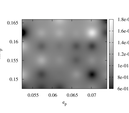
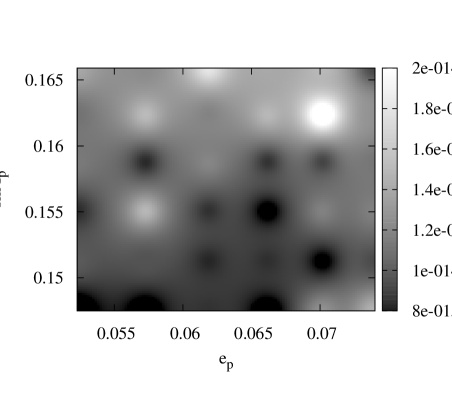
The above results suggest that the (5,-2,-2) MMR is essentially the only resonance in the Veritas region characterized by appreciable macroscopic diffusion. We now focus on the variation of the diffusion coefficients with respect to $(e_{p},\sin I_{p})$ along this resonance. As shown in Fig. 6, the dependence of the diffusion rate on the initial values of the actions is very complex. The values of $D(J_{1})$ vary from (0.60$\pm 0.01$)$\times 10^{-14}$ yr^-1 to (1.66$\pm 0.02$)$\times 10^{-14}$ yr^-1 while, for $D(J_{2})$, they vary from (0.63$\pm 0.02$)$\times 10^{-14}$ yr^-1 to (2.31$\pm 0.03$)$\times 10^{-14}$ yr^-1. Consequently, chaotic diffusion along this resonance can in principle produce asymmetric “tails” in the distribution of group-A members. Note, however, that the coefficients only vary by a factor of $2-3$ and that their average values are essentially the same as in Tsiganis et al. (2007).

3.1.2 The MCMC Simulations - Chronology of Veritas

We can now use the MCMC method to simulate the evolution and determine the age of the Veritas family, assuming that all the dynamically distinct groups originated from a single brake-up event. A set of six values ($a_{p}$,$J_{1}$,$J_{2}$,$P$,$\gamma$,$H$) is assigned to each random walker in the simulation. All bodies are initially distributed uniformly inside a region of predefined size in $\delta J_{i}(0)$ and semi-major axes in the range [3.172, 3.176]. The age of the family, ($\tau$), is defined as the time needed for $0.3\%$ of the random walkers to leave an ellipse in the ($J_{1},J_{2}$) plane, corresponding to a 3-$\sigma$ confidence interval of a 2-D Gaussian distribution. We note that, for Veritas, the mobility in semi-major axis due to Yarkovsky is very small and practically insignificant for what concerns the estimation of its age, since the family is young and distant from the Sun. For older families one should also define appropriate borders in $a_{p}$.

Using the values of the coefficients obtained above, and the values of $\sigma(J_{1})$=($2.31\pm 0.22$)$\times 10^{-4}$, $\sigma(J_{2})$=($3.97\pm 0.30$)$\times 10^{-4}$, calculated from the distribution of the real group A members, we simulate the spreading of group A and estimate its age. Of course, the model depends on some free parameters: the initial spread of the group in ($\delta J_{1}(0)$, $\delta J_{2}(0)$), the time-step, $dt$, and the number of random-walkers, $n$. Therefore, the dependence of the age, $\tau$, on these parameters was checked. Uncertainties in the values of the current borders of the group (i.e. the confidence ellipse) and the values of the diffusion coefficients were taken into account, when calculating the formal error in $\tau$.

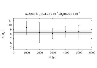
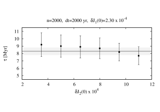
Different sets of simulations were performed, the results of which are given in Fig. 7(a)-(d). Each “simulation” (i.e. each point in a plot) actually consists of 100 different realizations (runs) of the MCMC code. In each run, the values of $D(J_{i})$ and $\sigma$($J_{i}$) were varied, according to the previously computed distributions of their values. The values of the free parameters were the same for all runs in a given simulation.

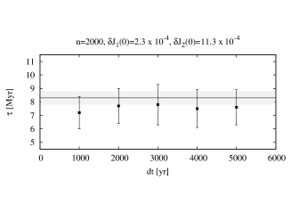
The first set of simulations was performed in order to check how the results depend on the time step, $dt$. Five simulations were made, with $dt$ ranging from 1000 to 5000 yr (Fig. 7a). The standard deviation of $\tau$ is relatively small, suggesting that $\tau$ is roughly independent of $dt$. According to this set of simulations, the age of the family is $\tau=\langle\tau\rangle\pm\Delta\tau=8.5\pm 1.3~{}$Myr, where $\langle\tau\rangle$ is the mean value and $\Delta\tau$ the standard error of the mean. This estimate is in excellent agreement with those of Nesvorný et al. (2003) and Tsiganis et al. (2007).

Figure 7: Dependence of $\tau$ and $\sigma(\tau)$ on three free parameters: (a) time step $dt$; (b) number of random walkers $n$; (c) initial size of the family $\delta J_{2}(0)$. The bottom panel, 7(d), shows the dependence of $\tau$ on $dt$ for a run in which the maximum values of $\delta J_{1}(0)$ and $\delta J_{2}(0)$ were assumed. The values of the free parameters that are constant in each group of simulations are indicated on top of each plot. The horizontal lines and dashed areas denote the age of the Veritas family (and the corresponding errorbar), as obtained by Nesvorný et al. (2003).

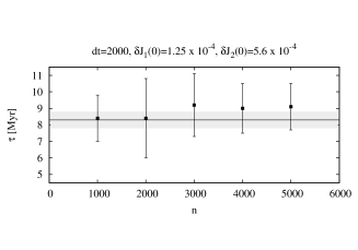
The second set of simulations was performed in order to check how the results depend on the number of random walkers, $n$. As shown in Fig. 7b), $\tau$ is weakly dependent of $n$, the variation of the mean value of $\tau$ is slightly larger than in the previous case. The age of the family, according to this set, is $\tau$ = 8.6$\pm$1.3 Myr.

The third group of simulations was performed in order to check how the results depend on the assumed initial spread of group A in $\delta J_{2}(0)$, a parameter which is poorly constrained from the respective equivelocity ellipse in Fig. 1. We fixed the value of $\delta J_{1}(0)$ to 2.3$\times 10^{-4}$, which can be considered an upper limit, according to Fig. (1). Six simulations were performed, with $\delta J_{2}(0)$ ranging from 3.5 $\times 10^{-4}$ to 11.0$\times 10^{-4}$, and the results are shown in Fig. 7c. The values of $\tau$ tend to decrease as $\delta J_{2}(0)$ increases. This is to be expected, since increasing the initial spread of the family, while targeting for the same final spread, should take a shorter time for a given diffusion rate. The results yield $\tau$ = 8.8$\pm$1.1 Myr.

As a final check, we performed a set of simulations with $\delta J_{1}(0)$ = 2.3$\times 10^{-4}$ and $\delta J_{2}(0)$ = 11.0$\times 10^{-4}$. These values correspond to equivelocity ellipses that contain almost all regular and (3,3,-2)-resonant family members, except for the very low inclination bodies ($\sin I_{p}<0.156$). Five sets of runs, for five different values of $dt$, were performed (see Fig. 7d). As in our first set of simulations, $\tau$ is practically independent of $dt$. On the other hand, $\tau$ turns out to be smaller than in the previous simulations, since the assumed values for $\delta J_{1}(0)$ and $\delta J_{2}(0)$ are quite large. Even so, we find $\tau$ = 7.6$\pm$1.1 Myr, which is still an acceptable value.

Combining the results of the first three sets of simulations and taking into account all uncertainties, we find an age estimate of $\tau$ = 8.7$\pm$1.2 Myr for the Veritas family. This result is very close to the one found by Tsiganis et al. (2007), the error though being smaller by $\sim 30\%$.

In addition to the determination of the family’s age, we would like to know how well the MCMC model reproduces the evolution of the spread of group-A bodies, in the ($J_{1}$,$J_{2}$) space. For this purpose we compared the evolution of group A for $10~{}$Myr in the future, as given (i) by direct numerical integration of the orbits, and (ii) by an MCMC simulation with variable diffusion coefficients. Figures 8(a)-(b) show the outcome of this comparison. As shown in Fig. 8(a), the random-walkers of the MCMC simulation (triangles) practically cover the same region in ($J_{1}$,$J_{2}$) as the real group-A members (circles). Moreover, the time evolution of the ratio of the standard deviations $\sigma(J_{2})/\sigma(J_{1})$, which characterizes the shape of the distribution, is reproduced quite well, as shown in Fig. 8(b).

An additional MCMC simulation with constant (i.e. average with respect to $e_{p}$ and $\sin I_{p}$) coefficients of diffusion was also performed. As shown in Fig. 8(b), the value of $\sigma(J_{2})/\sigma(J_{1})$ in this simulation appears to slowly deviate from the one measured in the previous MCMC simulation, as time progresses. However, this deviation is not very large, also compared to the result of the numerical integration. Thus, we conclude that an MCMC model with constant coefficients is adequate for deriving a reasonably accurate estimate of the age of a family, provided that the variations of the local diffusion coefficients are not very large. Given this result, we decided to use average coefficients for the Lixiaohua case. Note also that, in the Veritas case, the observed deviation in $\sigma(J_{2})/\sigma(J_{1})$ between the two MCMC models is reflected in the error of $\tau$ (i.e. 1.7 Myr vs. 1.2 Myr).

Figure 8: Comparison of the time evolution of group A Veritas members in (i) a numerical integration of their orbits for 10 Myr, and (ii) an MCMC realization, corresponding to the same time interval. Top: the final distribution, as taken from the integration (circles) and the MCMC run (triangles). Bottom: time evolution of the ratio $\sigma(J_{2})/\sigma(J_{1})$. The thick solid (resp. dashed) curve corresponds to the MCMC run with variable (resp. constant) diffusion coefficients, while the thin, “noisy” one corresponds to the numerical integration of the equations of motion.

3.2 The age of the Lixiaohua family

The Lixiaohua family is another typical outer-belt family, crossed by several MMRs. This results into a significant component of family members that follow chaotic trajectories. At the same time, a clear ‘V’-shaped distribution is observed in the $(a_{p},H)$ plane (see Fig. 9), suggesting that the family is old-enough for Yarkovsky to have significantly altered its size in $a_{p}$. Nesvorný et al. (2005) in this way estimated the age of this family to $\tau=300\pm 200~{}$Myr. Thus, we choose to study the Lixiaohua family because, on one hand, it is relatively old, so Yarkovsky/YORP effects are important, but, on the other hand, it has the feature we need (i.e. a significant chaotic zone) to test the behaviour of our model on longer time scales. Here, we use our MCMC method to derive a more accurate estimate of its age, taking into account also the Yarkovsky/YORP effects.

Figure 9: Top and middle panels: The same as Fig. 1, but for the Lixiaohua family. The different symbols correspond to different values of the Lyapunov time, $T_{L}$. Triangles correspond to $T_{L}>10^{5}~{}$y, empty circles to $2\times 10^{4}\leq T_{L}\leq 10^{5}~{}$y and solid circles to $T_{L}<2\times 10^{4}~{}$y. The equivelocity curves were obtained for $v=40$ m s^-1, $f=80^{\circ}$ and $\omega=300^{\circ}$. Bottom: The distribution of Lixiaohua members in the $(a_{p},H)$ plane. The grey-shaded region denotes the extent of the main chaotic zone (MCZ) in $a_{p}$. The two largest members of the family are also denoted.

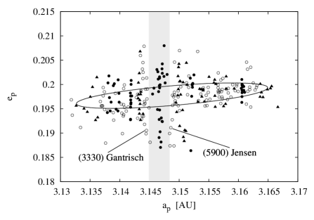
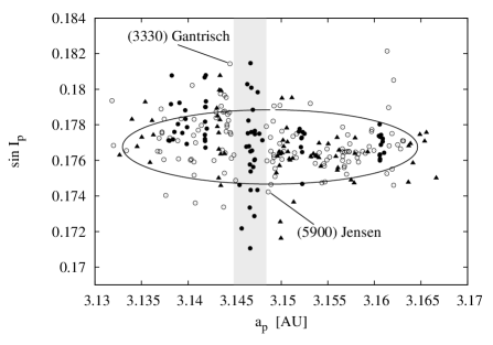
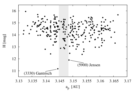
The distribution of the family members in $(a_{p},e_{p})$ and $(a_{p},\sin I_{p})$ is shown in Fig. 9. Using velocity cut-off $v_{c}=50~{}$m s^-1 we find 263 bodies (database as of February 2009) linked to the family. The shape of this family is, as in the Veritas case, intriguing. For $a>3.15~{}$AU, the family appears to better fit inside the equivelocity ellipse shown in the figure, with only a few bodies showing a significant excursion in $e_{p}$ and $\sin I_{p}$. On the other hand, for $a<3.145~{}$AU, the family members occupy a wider area in $e_{p}$ and $\sin I_{p}$. Throughout the family region we find thin, “vertical”, strips of chaotic bodies, with Lyapunov times $T_{L}<2\times 10^{4}~{}$y. These strips are associated to different mean motion resonances. The most important chaotic domain (hereafter Main Chaotic Zone, MCZ) is the one centered around $a_{p}\approx 3.146~{}$AU; indicated by the grey-shaded area in both plots of Fig. 9. A number of two- and three-body MMRs can be associated to the formation of the MCZ, such as the 17:8 MMR with Jupiter and the (7, 9, -5) three-body MMR.

Note that the two largest members of this family, (3330) Gantrisch and (5900) Jensen, are located just outside the MCZ, as indicated by their larger values of $T_{L}$ ($>2\times 10^{4}~{}$y). In fact, a significant group of bodies just outside the MCZ (see Fig. 9a) has higher values of $T_{L}$ but similar spread in $e_{p}$ as the MCZ bodies. This suggests that bodies around the chaotic zone could have once resided therein, evolving towards high/low values of $e_{p}$ by chaotic diffusion. Numerical integrations of the orbits of selected Lixiaohua members for 100 Myr indeed confirmed that bodies could enter (or leave) the MCZ. We believe that the distribution of family members on either side of the MCZ is strongly indicative of an interplay between Yarkovsky drift in semi-major axis and chaotic diffusion in $e_{p}$ and $\sin I_{p}$, induced by the overlapping resonances; bodies can be forced to cross the MCZ, thus receiving a “kick” in $e_{p}$ and $\sin I_{p}$, before exiting on the other side of the zone.

Figure 10: The same as Fig. 5, but for the Lixiaohua family. Note that while several diffusive peaks are visible in $D(J_{1})$, only the region of the MCZ ($a_{p}\sim 3.146~{}$AU) shows significant diffusion in $J_{2}$.

A population of $\approx 5,000$ fictitious bodies was selected and used for calculation of the local diffusion coefficients. Here, we restrict ourselves in calculating coefficients as functions of $a_{p}$ only (i.e. averaged in $e_{p}$ and $\sin I_{p}$). As shown in Fig. 10, there are several diffusive zones, corresponding to the low-$T_{L}$ strips of Fig. 9. However, as in the Veritas case, only one zone appears diffusive in both actions; $D(J_{2})$ is practically zero everywhere outside the MCZ ($a\sim 3.146~{}$AU), and significant dispersion in proper elements is observed only in this zone.

Given the above results, we conclude that the MCZ family members can be used to estimate the age of the family, much like the Veritas (5,-2,-2) resonant bodies. Given the fact that random-walkers can drift in $a_{p}$, the way of computing the age is accordingly modified. A large number of random walkers, uniformly distributed across the whole family region (i.e. the equivelocity ellipses) is used. The simulation again stops when $0.3\%$ of MCZ-bodies are found to be outside the observed $(J_{1},J_{2})$ borders of the family. However, the number of MCZ bodies is not constant during the simulation, because bodies initially outside (resp. inside) the MCZ can enter (resp. leave) that region. Thus, the aforementioned percentage is calculated with respect to the corresponding number of MCZ bodies at each time-step.

The size of the MCZ in the space of proper actions is given by $\sigma(J_{1})=(8.49\pm 0.51)\times 10^{-4}$ and $\sigma(J_{2})=(3.17\pm 0.28)\times 10^{-4}$. In order to compute the age of the family we performed 2400 MCMC runs. This was repeated three times, for three different values of thermal conductivity (see above) and once more, neglecting the Yarkovsky effect. Given the uncertainty in determining the initial size of the family, we repeated the computations for two more sets of $\delta J_{1}(0),\delta J_{2}(0)$. The results of these computations are presented in Fig. 11. We find an upper limit of $\sim 230$ Myr for the age of the family and a lower limit of $\sim 100~{}$Myr. Taking into account only the runs performed for our “nominal” initial size and including the Yarkovsky effect, we find the age of Lixiaohua family to be $155\pm 36$ Myr. This value lies towards the lower end but comfortably within the range ($300\pm 200~{}$Myr) given by Nesvorný et al. (2005).

Figure 11: The age of Lixiaohua family, as measured by our MCMC runs. The mean value and standard deviation (error-bar) of the age are given, as functions of the assumed size of the initial equivelocity ellipse. Four sets of points are shown, corresponding to our estimate (i) including Yarkovsky and assuming different values of the thermal conductivity ($K=0.01=$ dotted line, $K=0.1=~{}$dashed line and $K=0.5=~{}$solid thin line), and (ii) neglecting Yarkovsky (thick solid line).

We note that, when the Yarkovsky effect is taken into account, the age of the family turns out to be longer by $\sim 30~{}$Myr (see also Fig. 11). This is a purely dynamical effect, related to the fact that bodies can drift towards the MCZ from the adjacent non-diffusive regions. However, as more bodies enter the MCZ near its center in $e_{p}$ and $\sin I_{p}$, it takes longer for 0.3% of random walkers to diffuse outside the confidence ellipse in $(e_{p},\sin I_{p})$. At the same time, bodies that are initially inside the MCZ can also drift outside, to lower/higher values of $a_{p}$, thus slowing down or even stop diffusing in $e_{p}$ and $I_{p}$. This also explains the large spread in $(e_{p},\sin I_{p})$ observed for family members located just outside the MCZ.

4 Conclusions

We have presented here a refined statistical model for asteroid transport, which accounts for the local structure of the phase-space, by using variable diffusion coefficients. Also, the model takes into account the long-term drift in semi-major axis of asteroids, induced by the Yarkovsky/YORP effects. This model can be applied to simulate the evolution of asteroid families, also giving rise to an advanced version of the ”chaotic chronology” method for the determination of the age of asteroid families.

We applied our model to the Veritas family, whose age is well constrained from previous works. This allowed us to assess the quality and to calibrate our model. We first analyzed the local diffusion characteristics in the region of Veritas. Our results showed that local diffusion coefficients vary by about a factor of $2-3$ across the $(e_{p},\sin I_{p})$ region covered by the (5,-2,-2) MMR. Thus, although local coefficients are needed to accurately model (by the MCMC method) the evolution of the distribution of group-A members, average coefficients are enough for a reasonably accurate estimation of the family’s age. We note though that the variable coefficients model reduces the error in $\tau$ by $\sim 30\%$, but requires a computationally expensive procedure. Using the variable coefficients MCMC model, we found the age of the Veritas family to be $\tau$ = (8.7$\pm$1.2) Myr; a result in very good agreement with that of Nesvorný et al. (2003) and Tsiganis et al. (2007).

We used our model to estimate also the age of the Lixiaohua family. This family is similar to the Veritas family in many respects; it is a typical outer-belt family of C-type asteroids, crossed by several MMRs. Like the Veritas family, only the main chaotic zone (MCZ) shows appreciable diffusion in both eccentricity and inclination. On the other hand, this is a much older family and the Yarkovsky effect can no longer be ignored. This is evident from the distribution of family members, adjacent to the MCZ. Our model suggests that the age of this family is between 100 and 230 Myr, the best estimate being $155\pm 36~{}$Myr. Note that the relative error is $\approx 23\%$, i.e. close to the $\approx 20\%$ that Tsiganis et al. (2007) found for the Veritas case, using a constant coefficients MCMC model.

Our model shares some similarities with the Yarkovsky/YORP chronology. Both methods are basically statistical and make use of the quasi-linear time evolution of certain statistical quantities (either the spread in $\Delta a$ or the dispersion in $e_{p}$ and $\sin I_{p}$), describing a family. There are, however, important differences. The Yarkovsky/YORP chronology method works better for older families and the age estimates are more accurate for this class of asteroid families (provided there are no other important effects on that time scale). On the other hand, for our method to be efficient, we need that diffusion is fast enough to cause measurable effects, but slow enough so that most of the family members are still forming a robust family structure (i.e. there is no dynamical “sink” that would lead to a severe depletion of the chaotic zone). Thus, our model can be applied to a limited number of families that reside in complex phase-space regions, but, in the same time, this is the only model that takes into account the chaotic dispersion of these families. There are at least a few families for which both chronology methods can be applied, thus leading to more reliable age estimates, as well as to a direct comparison of the two different chronologies. For example, the families of (20) Massalia and (778) Theobalda would be good test cases. We, however, reserve this for future work.

An important advantage of the model is that it can be used to estimate the physical properties of a dynamically complex asteroid family, provided that its age is known by independent means (e.g. by applying the method of Nesvorný et al. (2003) to the regular members of the family). A large number of MCMC runs can be performed at low computational cost, thus allowing a thorough analysis of the physical parameters of family members or the properties of the original ejection velocities field that better reproduce the currently observed shape of the family.

References

- Beaugé & Roig (2001) Beaugé, C., Roig, F., 2001, Icarus, 153, 391
- Bendjoya & Zappalà (2002) Bendjoya, Ph., Zappalà, V., 2002, in: W. F. Bottke Jr., A. Cellino, P. Paolicchi, and R. P. Binzel (eds.), Asteroids III, University of Arizona Press, Tucson, 613
- Berg (2004) Berg, A.B., 2004, Markov Chain Monte Carlo Simulations and Their Statistical Analysis, World Scientific, Singapore
- Bottke et al. (2005) Bottke, W.F., Durda, D.D., Nesvorný, D., Jedicke, R., Morbidelli, A., Vokrouhlickỳ, D., Levison, H.F., 2005, Icarus 179, 63
- Brož et al. (2005) Brož, M., Vokrouhlický, D., Roig, F., Nesvorný, D., Bottke, W.F., Morbidelli, A., 2005, MNRAS, 359, 1437
- Brož (2006) Brož, M., 2006, Yarkovsky effect and the dynamics of Solar system. Ph.D. Thesis, Faculty of Mathematics and Physics, Charles University, Prague.
- Brown et al. (2007) Brown, M.E., Barkume, K.M., Ragozzine, D., Schaller, E.L., 2007, Nature, 446, 294
- Čapek & Vokrouhlický (2004) Čapek, D., Vokrouhlický, D., 2004, Icarus, 172, 526
- Carruba et al. (2003) Carruba, V., Burns, J.A., Bottke, W.F., Nesvorný, D., 2003, Icarus 162, 308
- Cellino et al. (2002) Cellino, A., Bus, S.J., Doressoundiram, A., Lazzaro, D., 2002, in: W. F. Bottke Jr., A. Cellino, P. Paolicchi, and R. P. Binzel (eds.), Asteroids III, University of Arizona Press, Tucson, 633
- Di Martino et al. (1997) Di Martino, M., Migliorini, F., Zappal, V., Manara, A., Barbieri, C., 1997, Icarus, 127, 112
- Donnison (2003) Donnison, J.R., 2003, MNRAS, 338, 452
- Durda et al. (2007) Durda, D.D., Bottke, W.F., Nesvorný, D., Enke, B.L., Merline, W.J., Asphaug, E., Richardson, D.C., 2007, Icarus, 186, 498
- Farinella & Vokrouhlický (1999) Farinella, P., Vokrouhlickỳ, D., 1999, Science, 283, 1507
- Farley et al. (2006) Farley, K.A., Vokrouhlický, D., Bottke, W.F., Nesvorný, D., 2006, Nature, 439, 295
- Gentle (2003) Gentle, E.J., 2003, Random Number Generation and Monte Carlo Methods. Springer, New York.
- Hirayama (1918) Hirayama, K., 1918, Astron. J., 31, 185
- Knežević & Milani (2000) Knežević, Z., Milani, A., 2000, Cel. Mech. Dyn. Astron., 78, 17
- Knežević & Pavlović (2002) Knežević, Z., Pavlović, R., 2002, Earth Moon Planets 88, 155
- Kryszczyńska et al. (2007) Kryszczyńska, A., La Spina, A., Paolicchi, P., Harris, A. W., Breiter, S., Pravec, P., 2007, Icarus, 192, 223
- Lazzaro et al. (2004) Lazzaro, D., Angeli, C.A., Carvano, J.M., Mothé-Diniz, T., Duffard, R., Florczak, M., 2004, Icarus, 172, 179
- Lichtenberg & Lieberman (1983) Lichtenberg, A.J., Lieberman, M.A. 1983. Regular and Stochastic Motion. Springer- Verlag New York, N.Y., U.S.A.
- Michel et al. (2003) Michel, P., Benz, W., Richardson, D.C., 2003, Nature, 421, 608
- Milani (1993) Milani, A., 1993, Cel. Mech. Dyn. Astron., 57, 59
- Milani & Farinella (1994) Milani, A., Farinella, P., 1994, Nature 370, 40
- Milani & Knežević (1990) Milani, A., Knežević, Z., 1990, Cel. Mech. Dyn. Astron., 98, 211
- Milani & Knežević (1994) Milani, A., Knežević, Z., 1994, Icarus, 107, 219
- Mothé-Diniz et al. (2005) Mothé-Diniz, T., Roig, F., Carvano, J.M., 2005, Icarus, 174, 54
- Morbidelli et al. (1995) Morbidelli, A., Zappalà, V., Moons,M., Cellino, A., Gonczi, R., 1995, Icarus 118, 132
- Morbidelli (2002) Morbidelli, A., 2002, Modern Celestial Mechanics: Aspects of Solar System Dynamics. Taylor & Francis, London.
- Murray & Holman (1997) Murray, N., Holman, M., 1997, Astron. J., 114, 1246
- Nesvorný & Morbidelli (1999) Nesvorný, D., Morbidelli, A., 1999, Celest. Mech. Dynam. Astron., 71, 243
- Nesvorný et al. (2002) Nesvorný, D., Bottke, W.F., Dones, L., Levison, H.F., 2002, Nature, 417, 720
- Nesvorný et al. (2003) Nesvorný, D., Bottke, W.F., Levison, H.F., Dones, L., 2003, Astrophys. J., 591, 486
- Nesvorný et al. (2005) Nesvorný, D., Jedicke, R., Whiteley, R.J., Ivezić, Ž., 2005, Icarus 173, 132
- Nesvorný et al. (2006) Nesvorný, D., Bottke, W.F., Vokrouhlický, D., Morbidelli, A., Jedicke, R., 2006, in: Daniela, L., Sylvio Ferraz, M., and Angel, F. Julio (eds.) Proceedings of the 229th Symposium of the IAU, Asteroids, Comets, Meteors, Cambridge University Press, Cambridge, 289
- Paolicchi et al. (1996) Paolicchi, P., Verlicchi, A., Cellino, A., 1996, Icarus, 121, 126
- Tedesco et al. (2002) Tedesco, E.F., Noah, P.V., Noah, M., Price, S.D., 2002, Astron. J., 123, 1056
- Tsiganis et al. (2003) Tsiganis, K., Varvoglis, H., Morbidelli, A., 2003, Icarus 166, 131
- Tsiganis et al. (2007) Tsiganis, K., Knežević, Z., Varvoglis, H., 2007, Icarus, 186, 484
- Vokrouhlický (1999) Vokrouhlický, D., 1999, Astron. Astrophys., 344, 362
- Vokrouhlický & Čapek (2002) Vokrouhlický, D., Čapek, D., 2002, Icarus, 159, 449
- Vokrouhlický et al. (2006a) Vokrouhlický, D., Brož, M., Morbidelli, A., Bottke, W.F., Nesvorný, D., Lazzaro, D., Rivkin, A.S., 2006, Icarus, 182, 92
- Vokrouhlický et al. (2006b) Vokrouhlický, D., Brož, M., Bottke, W.F., Nesvorný, D., Morbidelli, A., 2006, Icarus, 182, 118
- Zappal et al. (1995) Zappal, V., Bendjoya, Ph., Cellino, A., Farinella, P., Froeschl, C., 1995, Icarus, 116, 291