The two- and three-point correlation functions of the polarized five-year WMAP sky maps
Abstract
We present the two- and three-point real space correlation functions of the five-year WMAP sky maps and compare the observed functions to simulated CDM concordance model ensembles. In agreement with previously published results, we find that the temperature correlation functions are consistent with expectations. However, the pure polarization correlation functions are acceptable only for the 33GHz band map; the 41, 61, and 94 GHz band correlation functions all exhibit significant large-scale excess structures. Further, these excess structures very closely match the correlation functions of the two (synchrotron and dust) foreground templates used to correct the WMAP data for galactic contamination, with a cross-correlation statistically significant at the confidence level. The correlation is slightly stronger with respect to the thermal dust template than with the synchrotron template.
Subject headings:
cosmic background radiation — cosmology: observations — methods: numerical1. Introduction
Observations of the cosmic microwave background (CMB) have been among the most important ingredients in the revolution of cosmology that has taken place in the last two decades, when cosmology changed from a data starved to a data rich science. The so far most influential observations have been made with the Wilkinson Microwave Anisotropy Probe (WMAP; Bennett et al. 2003a; Hinshaw et al. 2007, 2009) satellite experiment, which has measured the microwave sky at five different frequencies (23, 33, 41, 61, and 94 GHz) in both temperature and polarization. Its main results are five sky maps with resolutions between and , each comprising more than three million pixels in each of the three Stokes parameters I, Q, and U.
The detector technology leading to instruments like WMAP has thus been very important in observing the CMB. Almost equally important has been the progress in computer technology and algorithms. With the enormously increased number of pixels from new high-resolution instruments, scientists have had to develop clever algorithms for every step of the required data analysis pipeline: map making (e.g., Ashdown et al. 2007; Hinshaw et al. 2003b, and references therein), component separation (e.g., Bennett et al. 2003b; Leach et al. 2008; Eriksen et al. 2008, and references therein), power spectrum and cosmological parameter estimation (e.g., Górski 1994; Lewis & Bridle 2002; Hivon et al. 2002; Hinshaw et al. 2003a; Verde et al. 2003; Eriksen et al. 2004d, and references therein), and analysis of higher-order statistics (e.g., Hinshaw et al. 1994; Kogut et al. 1995; Komatsu et al. 2003; Eriksen et al. 2004c, 2005 and references therein).
In this paper, we revisit a well-known example of the latter category, namely, real-space -point correlation functions. These functions arise naturally in studies of non-Gaussianity, since it can be shown that any odd-ordered -point function has an identically vanishing expectation value, while all even-ordered -point functions have an expectation value given by products of the corresponding two-point functions. Violation of either of these relations would indicate the presence of a non-Gaussian component in the field under consideration.
Earlier -point correlation function analyses of CMB data include studies of the COBE-DMR data (Hinshaw et al., 1995; Kogut et al., 1996; Eriksen et al., 2002), the WMAP temperature data (Eriksen et al., 2005) and one single two-point analysis of the first-year WMAP polarization data (Kogut et al., 2003). This paper is the first to consider the much more mature five-year WMAP polarization data, and the first to compute the three-point correlation function from any CMB polarization data. To do this, we adopt and extend the -point algorithms developed by Eriksen et al. (2004b).
2. Methods and definitions
2.1. -point correlation functions
An -point correlation function of a stochastic field is defined as
| (1) |
where spans an -polygon defined by parameters, . In the most general case in which no assumptions are made concerning the statistical properties of the field , one needs parameters to uniquely describe such a polygon111In this paper, we restrict our interest to fields defined on the two-dimensional sphere., namely, the individual positions of each vertex of the polygon. However, in many applications one assumes that is isotropic and homogeneous, and one can therefore average over position. In such cases, the number of parameters are reduced by three on a two-dimensional surface, corresponding to translation and rotation.

In this paper, we will consider only two- and three-point correlation functions defined on the two-dimensional sphere, and we therefore need, respectively, one and three parameters to describe our polygons (ie., line and triangle). In the two-point case, the only natural parameter choice is the angular distance, between the two points, while in the three-point case there is some freedom to choose. For simplicity, we parameterize the triangle by the lengths of the three edges, , where the edges are ordered such that corresponds to the longest of the three edges, and the remaining are listed according to clockwise traversal of the triangle.
2.2. Polarized correlation functions
Our goal in this paper is to measure the -point correlation functions of the polarized WMAP maps. To do so, we have to generalize the methods described by Eriksen et al. (2004b), in order to account for the fact that the CMB polarization field is a spin-2 field. Explicitly, the full CMB fluctuation field may be described in terms of the three Stokes parameters, I(), Q(), and U(). Here I is the usual (scalar) temperature fluctuation field, and Q and U are two parameters describing the linear polarization properties of the radiation in direction .
According to standard CMB conventions, Q and U are defined with respect to the local meridian of the spherical coordinate system of choice. However, Q and U form a spin-2 field, and this means that if one performs a rotational coordinate system transformation, the Stokes parameters after transformation becomes
| (2) |
where is the local rotation angle between the two coordinate systems. Zaldarriaga & Seljak (1997) and Kamionkowski et al. (1997) give complete descriptions of the statistics of these fields.
This property has some important consequences when computing -point correlation functions: since we assume that the CMB field is isotropic and homogeneous, the value we obtain for a given element of the correlation function should not depend on the coordinate system. One cannot therefore blindly adopt Q and U as the quantities to correlate, since these are in fact coordinate dependent.
For the two-point function, this problem is conventionally solved by defining a local coordinate system in which the local meridian passes through the two points of interest (Kamionkowski et al., 1997). The Stokes parameters in this new “radial” system are denoted by Qr and Ur, and measure the polarization either orthogonally or perpendicularly (Qr) to the connecting line, or 45∘ rotated with respect to it (Ur). The two-point function defined in terms of Qr and Ur then becomes coordinate system independent.
We now generalize this idea to higher-order -point correlation functions. As with the definition of the -point polygon parameters, we also here have some freedom when choosing the reference points for the coordinate independent quantities. For instance, two natural choices for Q and U are to define them either with respect to the edges or with respect to the center of mass of the polygon,
| (3) |
In this paper we choose the latter definition. The resulting geometry is illustrated in Figure 1.
Given these new rotationally invariant quantities, , defined with respect to the local center of mass, the polarized correlation functions are simply defined as
| (4) |
Note that in the case of the two-point function, there are six independent polarized correlation functions (II, IQr, IUr, QrQr, QrUr and UrUr), while in the three-point function case, there are 27 independent components (III, IIQr, , UrUrQr, UrUrUr).
Algorithmically, we compute these functions from a given pixelized sky map, , simply by averaging the corresponding products over all available pixel multiplets that satisfy the geometrical constraints of the polygon under consideration,
| (5) |
Here runs over the number of available pixel multiplets, and is the ’th pixel in the ’th pixel multiplet. For full details on how to find the relevant pixel multiplets corresponding to a given polygon efficiently, see Eriksen et al. (2004b).
The correlation functions are binned with a bin size tuned to the pixel size of the map. Explicitly, since we use a HEALPix resolution of , with pixels, we adopt a bin size of , for a total of 30 bins between and .
If all factors in an -point multiplet are taken from the same map, the resulting function is named an auto-correlation; otherwise, it is called a cross-correlation. The main advantage of cross-correlations is that the noise is typically uncorrelated between maps, while the signal (ideally) is strongly correlated. Therefore, the noise contribution to a cross-correlation averages to zero. For this reason, one typically uses auto-correlations as a probe of systematic errors (e.g., to check whether the assumed noise model is correct), but cross-correlations for a final cosmological analysis. In this paper, we consider both types.
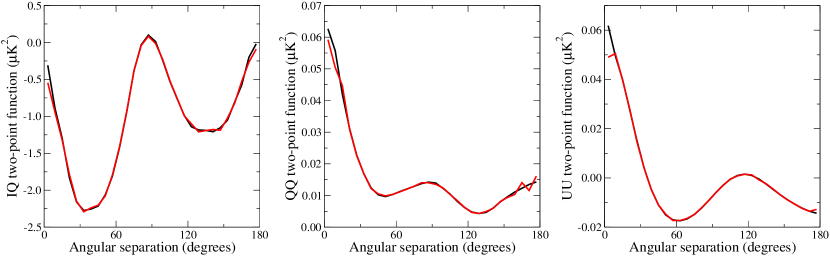
In Figure 2, we show a comparison of three two-point correlation functions computed from the same signal-only simulation, using two different methods: the red curves show the correlation functions computed from the power spectrum of the realization, employing the analytic expression given by, e.g., Smith (2006). The black curves show the correlation functions computed directly from the pixelized map using the algorithms described above. Slight differences are expected due to different treatment of pixel windows, but clearly the agreement between the two are excellent, giving us confidence that our machinery works as expected.
2.3. Comparison with simulations
In this paper we perform a standard frequentist analysis, in the sense that we compare the results obtained from the real data with an ensemble of simulations based on some model. Specifically, our null-hypothesis here is that the universe is isotropic and homogeneous, and filled with Gaussian fluctuations drawn from a CDM power spectrum. Our ensemble consists of simulations.
For each realization in the ensemble, we compute the -point correlation functions in precisely the same manner as for the real data. Finally, we compare the correlation function derived from the data with the simulated functions through a standard statistic,
| (6) |
where the sum runs over all -point configurations/bins, and the mean and variance are derived from the simulations.
However, before computing the as described above, we Gaussianize the distribution of each bin as follows (Eriksen et al., 2005):
| (7) |
where is the rank of the value under consideration (i.e., the number of simulations with a lower value than the currently considered), and is the corresponding Gaussianized rank. The reason for performing this transformation is that the probability distribution for a given bin is highly non-Gaussian, and for even-ordered correlation functions strongly skewed toward high values. A direct evaluation will therefore tend to give too much weight to fluctuations that have high values compared to fluctuations that have low values. By first explicitly Gaussianizing, a symmetric response is guaranteed.
| Correlation | |||||||||
|---|---|---|---|---|---|---|---|---|---|
| Frequency | II | IQ | IU | QI | QU | UI | UQ | UU | |
| KQ85 | |||||||||
| x | — | — | — | — | 0.40 (0.32) | 0.45 (0.38) | — | … | 0.32 (0.25) |
| x | 0.08 | 0.85 | 0.65 | … | 0.01 (348∗) | 0.01 (0.01) | … | … | 254∗ (128∗) |
| x | 0.07 | 0.26 | 0.61 | 0.85 | 25∗ (18∗) | 0.06 (0.04) | 0.69 | 0.01 (338∗) | 0.04 (0.02) |
| x | — | 0.81 | 0.97 | — | 0.01 (307∗) | 0.02 (0.01) | — | 0.03 (0.02) | 154∗ (48∗) |
| x | 0.08 | 0.84 | 0.05 | 0.86 | 3∗ (5∗) | 0∗ (0∗) | 0.69 | 0∗ (0∗) | 253∗ (222∗) |
| x | 0.07 | 0.27 | 0.60 | … | 73∗ (49∗) | 0.02 (0.01) | … | … | 0.01 (393∗) |
| x | — | 0.82 | 0.97 | — | 0.01 (357∗) | 21∗ (15∗) | — | 18∗ (10∗) | 0.02 (0.02) |
| x | 0.07 | 0.84 | 0.05 | 0.27 | 1∗ (2∗) | 42∗ (14∗) | 0.57 | 37∗ (8∗) | 106∗ (88∗) |
| x | — | 0.78 | 0.98 | — | — | — | — | — | — |
| x | 0.07 | 0.83 | 0.05 | … | 3∗ (0∗) | 71∗ (34∗) | … | … | 2∗ (0∗) |
| x | 0.09 | 0.70 | 0.11 | … | 116∗ (123∗) | 0.01 (0.01) | … | … | 5∗ (6∗) |
| x | 0.07 | 0.32 | 0.22 | … | 95∗ (83∗) | 0.03 (0.03) | … | … | 478∗ (476∗) |
| x | 0.07 | 0.91 | 0.82 | … | 0.78 (0.78) | 0.94 (0.94) | … | … | 0.60 (0.60) |
| x | 0.10 | 0.53 | 0.03 | … | 0∗ (0∗) | 0.08 (0.08) | … | … | 1∗ (3∗) |
| KQ75 | |||||||||
| x | 0.07 | 0.96 | 0.61 | … | … | … | … | … | … |
| x | 0.06 | 0.30 | 0.67 | 0.97 | … | … | 0.62 | … | … |
| x | — | 0.87 | 0.95 | — | … | … | — | … | … |
| x | 0.06 | 0.91 | 0.15 | 0.97 | … | … | 0.64 | … | … |
| x | 0.06 | 0.31 | 0.65 | … | … | … | … | … | … |
| x | — | 0.88 | 0.96 | — | … | … | — | … | … |
| x | 0.06 | 0.92 | 0.16 | 0.32 | … | … | 0.62 | … | … |
| x | — | 0.85 | 0.96 | — | — | — | — | — | — |
| x | 0.06 | 0.92 | 0.15 | … | … | … | … | … | … |
| x | 0.08 | 0.68 | 0.16 | … | … | … | … | … | … |
| x | 0.06 | 0.33 | 0.35 | … | … | … | … | … | … |
| x | 0.06 | 0.93 | 0.94 | … | … | … | … | … | … |
| x | 0.10 | 0.57 | 0.10 | … | … | … | … | … | … |
Note. — Statistical significances for the two-point functions as computed from the WMAP data. For the differencing assemblies, the first-year maps were used. For the band data, the five-year co-added maps were used. The Monte Carlo uncertainty is 1%. The correlations using both the KQ85 and the KQ75 masks are shown. As the pure polarization correlations are insensitive to which I mask is being used, these are only displayed under the KQ85 header. An entry with ’…’ signifies that some other entry in the table contains the same information as that entry, while an entry with ’—’ indicates that the information in that entry was not computed. The listed ratios indicate the fraction of simulations with a higher than the observed data. The entries marked with an ’*’ signifies that the fraction is lower than the Monte Carlo uncertainty, but still larger than zero; consequently, the number of simulations (out of 100,000) with a higher than the observed data are shown instead for these entries. The entries in parenthesis are the significances of the noise-only hypothesis.
The final results are quoted as the fraction of simulations with a higher than the real data. By splitting the simulations into two disjoint sets, and repeating the analysis for each set, we estimate that the Monte Carlo uncertainty in the resulting significances is less than 1%. For this reason, we quote cases inconsistent with simulations at more than 99% by instead providing the actual number of simulations with higher . This allows us to distinguish between a case with 1% significance and one with % significance, but still recognize the importance of the Monte Carlo uncertainties. Further, we conservatively never claim to obtain results with higher significance than 99% in any case, despite the fact that many results very likely are far more anomalous, as would be clear by using more simulations.
3. Data and simulations
In the following, we analyze the five-year WMAP sky maps, including both temperature and polarization. These data are available from LAMBDA222http://lambda.gsfc.nasa.gov, including all ancillary data, such as beam transfer functions, noise covariance matrices and foreground templates. The total data set spans five frequencies (23, 33, 41, 61, and 94 GHz), corresponding to the , , , , and bands.
Our main objects of interest are the frequency co-added and foreground-reduced sky maps, which are provided in the form of HEALPix333http://healpix.jpl.nasa.gov pixelized sky maps. The temperature sky maps are given at a HEALPix resolution of , while the polarization maps are given at . To bring the data into a common format, we therefore degrade the temperature component to the same resolution as the polarization maps, simply by averaging over sub-pixels in a low-resolution pixel.
For temperature we consider the , , and bands, and for polarization also the band. This difference mirrors the official cosmological WMAP analysis, which also uses the band for polarization, but considers the same band to be too foreground contaminated in temperature.
Our simulations are generated as follows: we first draw a random Gaussian CMB realization from the best-fit five-year WMAP CDM power spectrum, including multipole moments up to . This realization is then convolved with the instrumental beam of each WMAP differencing assembly and the HEALPix pixel window, and projected onto a HEALPix grid. For temperature, we then add a Gaussian noise realization with pixel-dependent variance, , where is the noise variance per observation and is the number of observations in that given pixel. The temperature component is then degraded to .
For the polarization component, we first degrade the high-resolution map to , and then add a noise term. This is because the polarized noise description for WMAP is given by a full noise covariance matrix, at , and not as a simple count at high resolution. The correlated noise realization is generated by drawing a vector of standard normal variates, , and multiplying this vector by the Cholesky factor of the covariance matrix, , where .
For temperature, we adopt two different masks, namely the five-year WMAP KQ85 and KQ75 masks. These exclude 18% and 28% of the sky, respectively. For the polarization component, there is only one relevant mask in the five-year WMAP data release, which excludes 27% of the sky.
Two different polarized foreground templates are used in the following. The first is simply the difference between the and bands, smoothed to an effective resolution of to reduce noise, which traces synchrotron radiation. The second template is the same starlight template as used for foreground correction in the five-year WMAP data release, which traces thermal dust.
4. Results
In this section we present the two- and three-point correlation functions computed from the polarized five-year WMAP data. Due to the large number of available and unique correlation functions one can form within this data set, we plot only a few selected cases, and instead show the full set of results only in the form of tabulated significances.
4.1. Two-point correlations
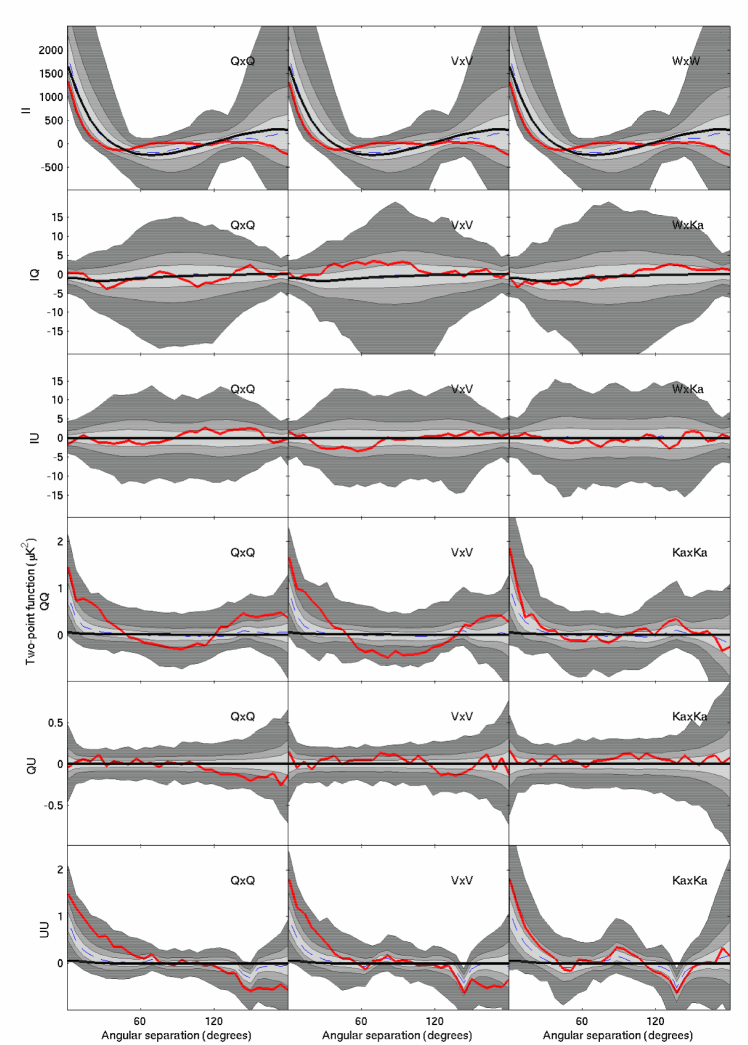
In Figure 3, we show a selection of two-point correlation functions derived from the WMAP data. Specifically, all available , and auto-correlations are shown, in addition to the cross-correlations between the and bands. Table 1 shows the significances for all possible two-point functions from the available data. (Note that only unique combinations are actually shown; empty table cells indicate that the same combinations may be found elsewhere in the table. For example, IQ and QI are identical for auto-correlations, but different for cross-correlations.)
Starting with the pure intensity correlations shown in the top row of Figure 3, we recognize the by now well-known behavior of the CMB temperature two-point function, observed both by COBE (e.g., Bennett et al., 1994) and WMAP (e.g., Spergel et al., 2003): at small angular separations, it is slightly low compared to the CDM model, and at separations larger than , very close to zero. This peculiar behavior has attracted the interest of both experimentalists and theorists, and some have suggested that this could be the signature of a closed topological space. However, from the view of a simple test, this function remains consistent with the simplest CDM model at the 5%–10% level.
Next, looking at the temperature-polarization (I-Q/U) cross-correlations we see that the overall behavior of the -, , and band functions are quite different. This indicates that the WMAP data still are too noise dominated to extract high-sensitivity cosmological information from individual bands. This is also reflected in the second and third columns of Table 1, where there is a significant scatter between the different results. However, we do see that all results are in good agreement with the expectations, indicating that the noise model is satisfactory.
The three bottom rows of Figure 3 show the pure polarization correlation functions, which are the main target in this paper. And here we see several interesting features. First, we recognize a sharp feature in the UU correlation function at . This is the angular separation between the A- and B sides of the differential WMAP detectors, and it was also seen in the pure noise temperature two-point correlation function in the first-year WMAP data (Eriksen et al., 2005).
However, even more interesting is the overall very pronounced large-scale excesses seen in the QQ and UU functions: both the - and -band functions lie mostly within the - confidence regions, and the overall agreement with the simulations appears quite poor.
Again, this is strongly reflected in Table 1: all QQ correlations are anomalous at more than 99% confidence, and all UU correlations at more than 98% confidence. In the case of the band, which happens to be the most anomalous of any band, we have good reasons to expect such behavior. This band has a significantly higher knee frequency than any other band (Jarosik et al., 2003), with the 4 differencing assembly having the highest. As a result, the WMAP team has chosen not to use this band for cosmological analysis in polarization. But the anomalous behavior of the and bands is a priori not expected; these are used for cosmological analysis by the WMAP team and should be clean.
We have also generated an ensemble of noise-only simulations, and computed the two-point functions from these. The corresponding fractions are listed in parentheses in Table 1 for the pure polarization modes. Here we see that, generally speaking, the noise-only hypothesis performs almost, but not quite, as well as the signal-plus-noise hypothesis. This is simply due to the fact that the WMAP polarization data are strongly dominated by the correlated noise, and it is very difficult from a correlation function point of view to distinguish between a small signal component and a large-scale noise fluctuation.
4.1.1 Foreground cross-correlations
The anomalous behavior seen in the - and -band two-point functions clearly needs an explanation. And typically, when such unexpected behavior is observed, one of the the first issues to consider is residual foregrounds.
To check whether this may be a relevant issue, we first simply compute the cross-correlation functions between each of the three frequency bands (, , and ) and the two available foreground templates (synchrotron and dust). This is done both for the real WMAP data and the simulated ensembles, and the agreement between the (pure CMB noise) simulations and the WMAP data is again quoted in terms of a fraction.
The results from these calculations are as follows: for the band, we find that the significances are 0.51 and 0.24 for synchrotron and dust, respectively, indicating no significant foreground detection in this case. However, for the band the corresponding numbers are 0.05 and , corresponding to correlations statistically significant at and , respectively. For the band, the numbers are 0.05 and 0.02, significant at or more.
To study these foreground correlations further, we compute the two-point functions from the foreground templates directly, and fit these to the observed correlation functions with a single free amplitude for each template, and , by minimizing
Here, is the correlation function mean and is the covariance matrix, both quantities obtained from the noise simulations. The indices run over all possible pure polarization two-point bins (i.e., both angular bins and QQ, QU, and UU correlations).
The resulting best-fit amplitudes from this calculation for -, - and bands are shown in Table 2. Here, we again see that the -band amplitudes are generally significantly lower than those of the and bands. (Note that the uncertainties quoted in this table only include statistical errors, not systematic errors. The significances should therefore not be considered as true detection levels, but are only suggestive.)
| Synchrotron | Dust | |||
|---|---|---|---|---|
| Band | ||||
| 0.0038 | 2.9 | 0.0115 | 2.0 | |
| 0.0052 | 5.2 | 0.0256 | 6.1 | |
| 0.0063 | 5.7 | 0.0197 | 4.2 | |
Note. — Mean values and confidence intervals for the best-fit amplitudes of the and dust template two-point functions relative to the WMAP data two-point functions.
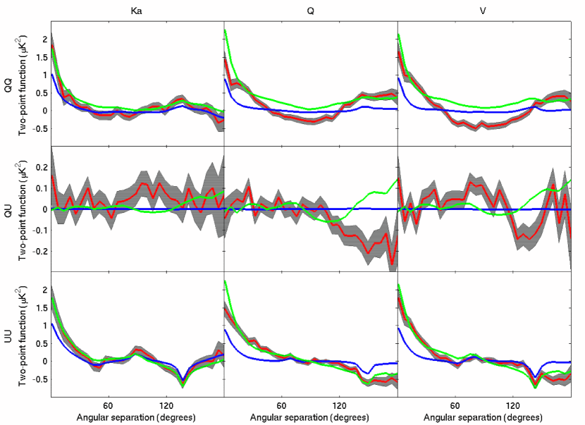
In Figure 4, the fitted correlation functions are compared to the observed functions. First, the red curve shows the functions derived from the actual WMAP data, with gray bands indicating the uncertainties derived from simulations. The blue curve shows the mean correlation function of the simulations, , and finally, the green curve shows the same, but with the foreground contribution added in, . Clearly, the latter matches the real data far better than the pure CMB-plus-noise hypothesis, with the best match seen in the UU correlation function.
4.2. Three-point correlations
| Correlation | ||||||||
|---|---|---|---|---|---|---|---|---|
| Frequency | QQQ | QQU | QUQ | QUU | UQQ | UQU | UUQ | UUU |
| Equilateral functions | ||||||||
| xx | 0.04 (0.03) | 0.31 (0.26) | 18∗ (4∗) | 0.04 (0.03) | 0.16 (0.13) | 0.01 (416∗) | 0.07 (0.05) | 0.21 (0.17) |
| xx | 0.45 (0.40) | 0.10 (0.08) | 0.07 (0.05) | 0.01 (446∗) | 359∗ (241∗) | 0.35 (0.31) | 0.01 (0.01) | 0.11 (0.09) |
| Collapsed functions | ||||||||
| xx | 0.49 (0.45) | 0.01 (0.01) | 0.23 (0.18) | 0.03 (0.02) | 0.63 (0.56) | 0.01 (384∗) | 0.21 (0.18) | 0.43 (0.38) |
| xx | 323∗ (240∗) | 0.01 (0.01) | 2∗ (1∗) | 0.05 (0.03) | 0∗ (1∗) | 0.11 (0.09) | 0.05 (0.03) | 17∗ (11∗) |
| xx | 0.01 (0.01) | 0.28 (0.25) | 0.01 (329∗) | 0.17 (0.14) | 0.01 (298∗) | 231∗ (179∗) | 0.07 (0.05) | 0.15 (0.12) |
| xx | 0.05 (0.04) | 0.09 (0.07) | 0.01 (0.01) | 0.10 (0.08) | 0.04 (0.03) | 0.07 (0.06) | 0.12 (0.09) | 0.12 (0.09) |
| xx | 0.21 (0.17) | 0.04 (0.03) | 180∗ (5∗) | 0∗ (2∗) | 3∗ (2∗) | 127∗ (79∗) | 80 (45∗) | 0.01 (456∗) |
| xx | 0.01 (0.01) | 0.03 (0.02) | 0.58 (0.51) | 439∗ (301∗) | 0.01 (0.01) | 0.38 (0.33) | 0.18 (0.13) | 0.05 (0.04) |
Note. — Statistical significances of the polarization-only three-point functions computed from the WMAP five-year co-added , and maps. The Monte Carlo uncertainty is 1%. See Table 1 for feature explanation.
We now turn to the three-point correlation functions derived from the five-year polarized WMAP data. However, we note that the three-point function is primarily used in the literature as a test of non-Gaussianity. In the present case, this will not be case, since we have already seen that the data appear to be foreground contaminated, and even the two-point correlation function fails a standard test. The following three-point analysis will therefore essentially only be a consistency check of the above results, and a demonstration of the general procedure, to be further developed in the future, when cleaner data become available.
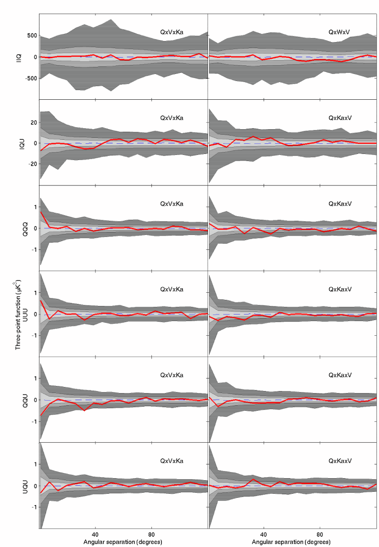
We consider only cross-correlations of pure polarization modes for the cosmologically interesting frequency channels. This leaves us with only eight independent correlation function modes (QQQ, QUQ, UQQ, UUU etc.), and only one frequency combination (). Further, we consider only two general types of three-point configurations, namely, equilateral and pseudo-collapsed triangles. The latter is defined such that two legs of the triangle are of equal length, while the third leg spans an angular distance of less than .
The results from these calculations are tabulated in Table 3, and a few arbitrarily chosen modes of the equilateral three-point functions are plotted in Figure 5. (Plotting all functions would take too much space, without adding any particular new insights.)
Once again, we see that the ’s obtained from the real data are high, but generally not quite as striking as in the two-point case. This is at least partly due to the fact that the band is involved in all configurations, as well as the fact that the three-point function is always “noisier” than the two-point function. We also see that the noise-only hypothesis always has higher ’s than the signal-plus-noise hypothesis, again following the two-point behavior.
It is difficult to interpret these results much further, given that there are clear problems already at the two-point level. We therefore leave a full interpretation of the three-point function to a future publication, when cleaner data, either from WMAP or Planck, have been made available.
5. Conclusions
We compute for the first time the polarized two- and three-point correlation functions from the five-year WMAP data, with the initial motivation of constraining possible non-Gaussian signals on large scales in the CMB polarization sector. However, our main result is a detection of a signature consistent with residual foregrounds in both the - and -band data, significant at -.
This should not come as a complete surprise, though, as a similar result was found in the three-year WMAP data through a direct template fit approach by Eriksen et al. (2007). They used a Gibbs sampling implementation to estimate the joint CMB power spectrum and foreground template posterior, and found non-zero template amplitudes at similar significance levels when marginalizing over the CMB spectrum. Given the results found in the present paper, this still appears to be an important issue for the five-year WMAP data release. Resolving this question is of major importance for the CMB community, since many cosmological parameters depend critically on the large-scale WMAP polarization data, most notably the optical depth of reionization, , and the spectral index of scalar perturbations, .
The question of primordial non-Gaussianity in CMB polarization data can not be meaningfully addressed as long as this issue is unresolved. The three-point correlation function results shown in this paper therefore mostly serve as a demonstration of the approach, and as a cross-check on the two-point results. The three-point function will obviously become a more important and independent quantity in the future, when higher-fidelity polarization data become available.
Appendix A Precomputing configuration tables
In order to compute the two-and-three point functions, we have utilized the method introduced by Eriksen et al. (2004b).
The basic idea of this method is that given the resolution and the mask of the map, and the desired number of distance bins, the configurations that correspond to an angle is uniquely determined. One may then do the work of finding these configurations only once, saving them in large tables. Each table then corresponds to a certain bin , and the first row in each table contains all the unmasked pixels of the map. Each column contains all pixels at a distance given by from the pixel in the first element of the column. By moving through a column in such a table, one then traces out a circle of radius . Thus, by saving the configurations in tables, one pays the initialization costs only once.
An additional, powerful feature of this approach becomes apparent when computing correlation functions of higher order than 2. If one thinks of these tables as compasses, tracing out circles of a given length for each pixel, it should be clear that, just as one can construct, e.g., triangles using compasses, one can construct triangles on the sphere using these tables. If the edges of the desired triangle is of lengths , and , one begins with the table, selects a pixel from the upper row, and selects a second pixel from the column below this pixel. One then has the baseline of the triangle. To construct a triangle with a compass when the baseline is given, one would adjust the compass so that it spans a length equal to the length of the second edge of the triangle, and draw a circle with this radius with one end of the baseline as the center of the circle. Then, one would again adjust the compass so that it spans the desired third length of the triangle, and draw a circle around the other end of the baseline. Then, one would check whether the two circles drawn intercept at any point(s). These points would then be the third vertex of the triangle. Carrying this analogy to our tables, our two already chosen pixels are the ends of the baseline around which to draw our circles. We ’adjust our compass’ by finding pixel 1 in the first row of table , we ’draw a circle around it’ by looping over all pixels in the column below it, and do the same for pixel 2, expect that we now look in table . By checking whether there are any common pixels in these ’circles’, we find the triangle(s) whose edges have the desired lengths.
Since any -point polygon can be reduced to triangles, higher-order correlation functions can also be computed using this method.
References
- Ashdown et al. (2007) Ashdown, M. A. J., et al. 2007, A&A, 467, 761
- Bennett et al. (1994) Bennett, C. L., et al. 1994, ApJ, 436, 423
- Bennett et al. (2003a) Bennett, C. L., et al. 2003a, ApJS, 148, 1
- Bennett et al. (2003b) Bennett, C. L., et al. 2003b, ApJS, 148, 97
- Eriksen et al. (2002) Eriksen, H. K., Banday, A. J., & Górski, K. M. 2002, A&A, 395, 409
- Eriksen et al. (2004a) Eriksen, H. K., Hansen, F. K., Banday, A. J., Górski, K. M., & Lilje, P. B. 2004a, ApJ, 605, 14
- Eriksen et al. (2004c) Eriksen, H. K., Novikov, D. I., Lilje, P. B., Banday, A. J., & Górski, K. M. 2004c, ApJ, 612, 64
- Eriksen et al. (2004b) Eriksen, H. K., Lilje, P. B., Banday, A. J., & Górski, K. M. 2004b, ApJS, 151, 1
- Eriksen et al. (2004d) Eriksen, H. K., et al. 2004d, ApJS, 155, 227
- Eriksen et al. (2005) Eriksen, H. K., Banday, A. J., Górski, K. M., & Lilje, P. B. 2005, ApJ, 622, 58
- Eriksen et al. (2007) Eriksen, H. K., Huey, G., Banday, A. J., Górski, K. M., Jewell, J. B., O’Dwyer, I. J., & Wandelt, B. D. 2007, ApJ, 665, L1
- Eriksen et al. (2008) Eriksen, H. K., Jewell, J. B., Dickinson, C., Banday, A. J., Górski, K. M., & Lawrence, C. R. 2008, ApJ, 676, 10
- Górski (1994) Górski, K. M. 1994, ApJ, 430, L85
- Górski et al. (2005) Górski, K. M., Hivon, E., Banday, A. J.,Wandelt, B. D., Hansen, F. K., Reinecke, M., Bartelman, M. 2005, ApJ, 622, 759
- Hinshaw et al. (1994) Hinshaw, G., et al. 1994, ApJ, 431, 1
- Hinshaw et al. (1995) Hinshaw, G., Banday, A. J., Bennett, C. L., Górski, K. M., & Kogut, A. 1995, ApJ, 446, L67
- Hinshaw et al. (2003a) Hinshaw, G., et al. 2003a, ApJS, 148, 135
- Hinshaw et al. (2003b) Hinshaw, G., et al. 2003b, ApJS, 148, 63
- Hinshaw et al. (2007) Hinshaw, G., et al. 2007, ApJS, 170, 288
- Hinshaw et al. (2009) Hinshaw, G., et al. 2009, ApJS, 180, 225
- Hivon et al. (2002) Hivon, E., Górski, K. M., Netterfield, C. B., Crill, B. P., Prunet, S., & Hansen, F. 2002, ApJ, 567, 2
- Jarosik et al. (2003) Jarosik, N., et al. 2003, ApJS, 148, 29
- Kamionkowski et al. (1997) Kamionkowski, M., Kosowsky, A., & Stebbins, A. 1997, Phys. Rev. D, 55, 7368
- Kogut et al. (1995) Kogut, A., Banday, A. J., Bennett, C. L., Hinshaw, G., Lubin, P. M., & Smoot, G. F. 1995, ApJ, 439, L29
- Kogut et al. (1996) Kogut, A., Banday, A. J., Bennett, C. L., Górski, K. M., Hinshaw, G., Smoot, G. F., & Wright, E. L. 1996, ApJ, 464, L29
- Kogut et al. (2003) Kogut, A., et al. 2003, ApJS, 148, 161
- Komatsu et al. (2003) Komatsu, E., et al. 2003, ApJS, 148, 119
- Leach et al. (2008) Leach, S. M., et al. 2008, A&A, 491, 597
- Lewis & Bridle (2002) Lewis, A., & Bridle, S. 2002, Phys. Rev. D, 66, 103511
- Smith (2006) Smith, K. M. 2006, Phys. Rev. D, 74, 083002
- Spergel et al. (2003) Spergel, D. N., et al. 2003, ApJS, 148, 175
- Verde et al. (2003) Verde, L., et al. 2003, ApJS, 148, 195
- Zaldarriaga & Seljak (1997) Zaldarriaga, M., & Seljak, U. 1997, Phys. Rev. D, 55, 1830