Phonon renormalization from local and transitive electron-lattice couplings in strongly correlated systems

Abstract

Within the time-dependent Gutzwiller approximation (TDGA) applied to Holstein- and SSH-Hubbard models we study the influence of electron correlations on the phonon self-energy. For the local Holstein coupling we find that the phonon frequency renormalization gets weakened upon increasing the onsite interaction $U$ for all momenta. In contrast, correlations can enhance the phonon frequency shift for small wave-vectors in the SSH-Hubbard model. Moreover the TDGA applied to the latter model provides a mechanism which leads to phonon frequency corrections at intermediate momenta due to the coupling with double occupancy fluctuations. Both models display a shift of the nesting-induced to a $q=0$ instability when the onsite interaction becomes sufficiently strong and thus establishing phase separation as a generic phenomenon of strongly correlated electron-phonon coupled systems.

I Introduction

Transition metal compounds are usually characterized by strong electron-electron and electron-phonon interactions (for an overview cf. Ref. maekawa, ). The interplay of these interactions can give rise to a large variety of interesting electronic properties which also reflect in the energy and momentum structure of the phonons. In this regard a well known phenomenon is the occurence of bond-stretching phonon anomalies which are observed in high-T_c cuprates La_2-xSr_xCuO₄queeney99 ; pintch99 and YBa${}_{2}2$Cu₃O_6+x,Reich96 HgBa₂CuO_4+δ,uchiyama04 Nd_1.86Ce_0.14CuO_4+δ,DAs02 Bi₂Sr_1.6La_0.4Cu₂O_6+δgraf08 but also in Pb- and K-doped BaBiO₃, braden02 Sr₂RuO₄, braden07 La_1.69Sr_0.31NiO₄ tran02 and La_1-xSr_xMnO₃.reich99

The interpretation of such experiments requires an understanding of the renormalization of phonons in a strongly correlated electron system which is the purpose of the present paper. Such an analyis is usually based on Hubbard-type models where the two most popular variants to implement an electron-lattice coupling are either to consider the dependency of onsite energies or of the hopping integrals as a function of some atomic coordinates. In the first case, when one restricts to the interaction between electron density and coordinate of the same lattice site, the coupling is usually termed a Holstein or molecular crystal model. hol59 In the second case, when the hopping between nearest-neighbor sites is expanded in terms of the positions of these sites the resulting electron-lattice coupling is often named after Su, Schrieffer and Heeger (SSH) which have used this type of interaction for the analysis of solitons in polyacetylene. ssh

Since lattice vibrations are partially screened by the electrons the latter can have a profound influence on the effective dispersion of the phonons. One example is the Kohn anomaly kohn caused by the abrupt change of electronic screening near wave-vectors ${\bf q}$ which are twice the Fermi momentum $k_{F}$ (nesting). Moreover, electronic correlations alter the electron dynamics of the system and thus also affect the phonon dispersion. In case of a Holstein coupling, and due to the fact that correlations reduce the charge correlations at $k_{F}$ in favor of an enhancement of the $q=0$ response, it has been shown Gri94 ; CDCG95 that the formation of a charge density wave (CDW) is suppressed in favor of a phase separation instability. For the phonons this has the immediate consequence that the softening is shifted from the Kohn anomaly wave-vector $q=2k_{F}$ to $q=0$.

Naturally the interplay between lattice and electronic degrees of freedom has already been investigated by means of several techniques. Some of the approaches, like quantum Monte Carlo, HS83 ; Hir83 ; HS84 ; Hir85 ; Ber95 ; srini ; Hua03 exact diagonalization, dob94 ; dob94epl ; lor94b ; stephan and Dynamical Mean Field Theory (DMFT) FJ95 ; Capo04 ; Kol04-1 ; Kol04-2 ; Jeo04 ; San05 ; San06 are intrinsically non-perturbative but are numerically challenging and suffer some limitations (small lattice sizes, no momentum resolution, etc.). On the other hand (semi)analytical approaches like variational ones, slave boson and large-N expansion baer85 ; tes93 ; Gri94 ; Kel95 ; Zey96 ; alder97 ; caprara ; Koc04 ; Cap04 ; Cit01 ; Cit05 deal with infinite systems, but within approximate treatments. It should be noted that most of the work has been done on the Hubbard-Holstein model. The papers which explicitely deal with an Hubbard-SSH model Hir83 ; srini ; baer85 ; tes93 ; alder97 ; caprara mainly focus on the interplay between correlations and dimerization or superconductivity, respectively.

In this paper we want to study the correlation effects on the phonon excitations for both Holstein and SSH models on the same footing. To this aim we need a method which is not numerically very demanding, but still provides a quantitatively acceptable treatment of the strongly correlated regime. In this regard we find the Gutzwiller approximation (GA) supplemented with RPA-type fluctuations, the so-called time-dependent GA (TDGA), a good compromise. This technique corresponds to Vollhardt’s Fermi liquid approachvol84 with the fluctuations extended to finite frequencies and momenta. Electron-phonon interactions will be treated in the Born-Oppenheimer approximation.

It is worth mentioning that the TDGA approach has been tested in various situations and found to be accurate compared with exact diagonalization. sei01 ; sei03 ; sei04b ; sei07b Computations for realistic models have provided a description of different physical quantities in agreement with experiment. lor02b ; lor03 ; sei05

In the discussion of results we will restrict to one-dimensional systems. This clearly simplifies the computations and the presentation of the results. It has the drawback that strictly one dimensional systems are those for which our Fermi liquid like approach is expected to be less suited. Thus our results should not be taken too literally in this case. On the other hand the qualitative behavior we find is rather independent of dimension. For example for the Holstein model we find here the same qualitative behavior for the charge response as we have found before in larger dimensions. diciolo08 Despite the inadequacy of a Fermi liquid treatment for strictly one dimensional systems several real systems are only quasi one dimensional and in those cases our computations can be applicable. We also found that in certain filling ranges the results are surprisingly accurate.

The scheme of our paper is as follows. In Sec. II we define the model and show how the Hubbard-Holstein and -SSH hamiltonians are represented within the GA. After introducing the TDGA in Sec. IIC the phonon self-energy for both Holstein- and SSH-couplings is derived in Sec. IID,E. In Sec. IIIA we first investigate the quality of our technique by comparing with exact and Monte-Carlo results in one dimension and furtheron present the results for the phonon self-energies of the Holstein- and SSH-Hubbard model in Secs. IIIB,C. Our conclusions can be found in Sect. VII and the details of our calculations are given in the Appendix.

II Formalism

II.1 Model

Our investigations are based on the following hamiltonian

$$H=H_{e}+H_{e-ph}+H_{ph}$$ (1)

where $H_{e}$ denotes the Hubbard model, $H_{e-ph}$ the coupling between electrons and phonons and $H_{ph}$ the bare phonon part. Here we restrict to one-dimensional systems and consider for the electronic part hopping between nearest neighbors

$$H_{e}=-t\sum_{i,\sigma}\left(c_{i,\sigma}^{\dagger}c_{i+1,\sigma}+c_{i+1,\sigma}^{\dagger}c_{i,\sigma}\right)+U\sum_{i}n_{i,\uparrow}n_{i,\downarrow}$$ (2)

where $c_{i,\sigma}^{(\dagger)}$ destroys (creates) an electron on lattice site $R_{i}$ and $n_{i,\sigma}=c_{i,\sigma}^{\dagger}c_{i,\sigma}$.

We consider two types of electron-phonon coupling. The first is a local Holstein interaction initially motivated from a molecular crystal model

$$H_{e-ph}^{hol}=-\alpha\sum_{i,\sigma}u_{i}\left(n_{i,\sigma}-\langle n_{i,\sigma}\rangle\right)$$ (3)

where $u_{i}$ is the coordinate of an internal mode of the molecules affecting the site energy at site $i$. Its dynamics is described by

$$H_{ph}^{hol}=\frac{1}{2}K\sum_{i}u_{i}^{2}+\frac{1}{2M}\sum_{i}p_{i}^{2}$$ (4)

and corresponds to dispersionless lattice modes. Here $K$, $M$ denote elastic constant and reduced mass and $p_{i}$ are the conjugate momenta at site $i$.

The second type of coupling originates from the dependence of the electronic hopping on the atomic coordinates. For the one-dimensional model under consideration this so-called SSH or Peierls interaction is given by

$$H_{e-ph}^{ssh}=-\alpha t\sum_{i,\sigma}\left(u_{i+1}-u_{i}\right)\left(c_{i,\sigma}^{\dagger}c_{i+1,\sigma}+c_{i+1,\sigma}^{\dagger}c_{i,\sigma}\right)$$ (5)

and in this case the lattice dynamics is determined from

$$H_{ph}^{ssh}=\frac{1}{2}K\sum_{i}\left(u_{i+1}-u_{i}\right)^{2}+\frac{1}{2M}\sum_{i}p_{i}^{2}.$$ (6)

II.2 Gutzwiller approximation

We treat the model Eq. (1) within the Gutzwiller approximation (GA) supplemented by Gaussian fluctuations the evaluation of which are outlined in the next section. The GA can either be motivated from a slave-boson approach Kot86 or a variational Ansatz formally evaluated in infinite dimensions. Geb90 The variational wave function is given by $|\Psi\rangle=\hat{P}|\phi\rangle$, where the Gutzwiller projector $\hat{P}$ acts on the Slater determinant $|\phi\rangle$. This approach incorporates the correlation induced renormalization of the kinetic energy and treats the Hubbard on-site interaction via the variational double occupancy parameters $D_{i}$. For each term in the Hamiltonian we derive an energy functional $E^{GA}[\rho,D]\equiv\langle\Psi|H|\Psi\rangle$ where we have introduced the one body density matrix associated with the Slater determinant $\rho_{i,j,\sigma}=\langle\phi|c_{i,\sigma}^{\dagger}c_{j,\sigma}|\phi\rangle$. Specifically the energy functional for the electronic part Eq. (2) reads as

$$E_{e}^{GA}[\rho,D] = -t\sum_{i,\sigma}z_{i,\sigma}z_{i+1,\sigma}\left(\rho_{i,i+1,\sigma}+\rho_{i+1,i,\sigma}\right)$$ (7)

$$+ U\sum_{i}D_{i}$$

and the $z$-factors are given by

$$z_{i\sigma}=\frac{\sqrt{(\rho_{ii,\sigma}-D_{i})(1-\rho_{ii}+D_{i})}+\sqrt{(\rho_{ii,-\sigma}-D_{i})D}_{i}}{\sqrt{\rho_{ii,\sigma}(1-\rho_{ii,\sigma})}}.$$ (8)

Further on $\rho_{ij}=\sum_{\sigma}\rho_{ij,\sigma}$.

Within the Born-Oppenheimer approximation the electronic expectation value of $H_{e-ph}$ determines the lattice potential. In contrast to the local Holstein coupling, for electronic degrees the transitive SSH electron-phonon interaction Eq. (5) is also renormalized by the z-factors and the corresponding energy functional reads as

$$E_{e-ph}^{ssh,GA} = -\alpha t\sum_{i,\sigma}\left(u_{i+1}-u_{i}\right)z_{i,\sigma}z_{i+1,\sigma}$$ (9)

$$\times \left(\rho_{i,i+1,\sigma}+\rho_{i+1,i,\sigma}\right).$$

The GA variational ground state is then obtained upon minimizing $E^{GA}$ with respect to $\{D\}$, $\{u\}$, and $\rho$ under the constraint that the latter derives from a Slater determinant, i.e. $\rho^{2}=\rho$. In the following our starting point will be an homogeneous state. The formation of possible charge-density wave (in case of the Holstein model) and dimerized (in case of the SSH model) states will appear as instabilities of the homogeneous state. Thus our initial ground state is characterized by $u_{i}\equiv 0$, $\rho_{ii,\sigma}\equiv\rho_{0}/2$, $D_{i}\equiv D_{0}$ and $z_{i}\equiv z_{0}$. The ground state energy per site is therefore simply determined from Eq. (7) and reads

$$E^{GA}[\rho,D]/N=z_{0}^{2}e_{0}+UD_{0}$$ (10)

and $e_{0}$ denotes the energy per site of a non-interacting system with charge density $\rho_{0}$. For later use we also denote the critical value of the onsite repulsion $U=U_{c}=32t/\pi$ for a half-filled one-dimensional chain at which the Brinkman-Rice transition (i.e. complete localization of the charge carriers with $D_{0}=0$) takes place.

II.3 Time-dependent Gutzwiller approximation

In order to study fluctuations beyond the GA saddle-point solution, necessary for the evaluation of the phonon self-energies, we use the time-dependent GA (TDGA) which has been developed in Refs. sei01, ; sei03, .

We briefly illustrate the formalism for the electronic part $H_{e}$ and furtheron show how lattice fluctuations can be implemented into the theory. Further details can be found in Refs. sei01, ; sei03, ; diciolo08, .

We study the response of the system to a small time dependent external field which produces time dependent fluctuations in the density matrix $\delta\rho$ and the double occupancy $\delta D$. This can then be obtained by expanding $E^{GA}$ up to quadratic order in the density and double occupancy fluctuations $\delta\rho$ and $\delta D$.

For a translationally invariant ground state it is convenient to perform the expansion in momentum space. Besides the local fluctuation $\delta\rho_{\bf q}$, we introduce the bond charge fluctuationdiciolo08 ,

$$\delta T_{i}=-t\sum_{\sigma\eta=\pm 1}(\delta\rho_{i+\eta,i,\sigma}+\delta\rho_{i,i+\eta,\sigma}).$$

It is convenient to introduce the hopping factor in the definition of $\delta T_{i}$ so that it can also be interpreted as a local kinetic energy. Notice however that the $z$ factors are omitted. The Fourier transform is given by

$$\delta T_{q}=-2t\sum_{k,\sigma}\left[\cos(k+q)+\cos(k)\right]\delta\rho_{k+q,k,\sigma}.$$ (11)

For latter use it is also convenient to introduce the antisymmetric combination of bond charge fluctuations:

$$\delta T_{i}^{-}=-t\sum_{\sigma\eta=\pm 1}\eta(\delta\rho_{i+\eta,i,\sigma}+\delta\rho_{i,i+\eta,\sigma}).$$

with Fourier transform:

$$\delta T_{q}^{-}=-2it\sum_{k,\sigma}\left[\sin(k+q)-\sin(k)\right]\delta\rho_{k+q,k,\sigma}.$$ (12)

It is easy to check that the two fluctuations are related by a function of $q$:

$$\delta T_{q}^{-}=i\tan\left(\frac{q}{2}\right)\delta T_{q}$$ (13)

The second order-energy expansion in the charge channel of Eq. (7) follows as:

$$E_{e}^{GA,(2)} = \frac{1}{N}\left[\frac{1}{2}\sum_{q}V_{q}\delta\rho_{q}\delta\rho_{-q}+z_{0}z_{D}^{\prime}\sum_{q}\delta D_{q}\delta T_{-q}\right.$$ (14)

$$+ \frac{1}{2}z_{0}(z^{\prime}+z_{+-}^{\prime})\sum_{q}\delta\rho_{q}\delta T_{-q}$$

$$+ \left.\sum_{q}L_{q}\delta\rho_{q}\delta D_{-q}+\frac{1}{2}\sum_{q}U_{q}\delta D_{q}\delta D_{-q}\right]$$

with the following definitions:

$$V_{q} = \frac{e_{0}z_{0}}{2}(z_{++}^{\prime\prime}+2z_{+-}^{\prime\prime}+z_{--}^{\prime\prime})+\frac{1}{2}(z^{\prime}+z_{+-}^{\prime})^{2}e_{0}\cos(q)$$

$$L_{q} = e_{0}z_{0}(z_{+D}^{\prime\prime}+z_{-D}^{\prime\prime})+z_{D}^{\prime}(z^{\prime}+z_{+-}^{\prime})e_{0}\cos(q)$$

$$U_{q} = 2e_{0}z_{0}z_{D}^{\prime\prime}+2(z_{D}^{\prime})^{2}e_{0}\cos(q)$$

where $z^{\prime}$ and $z^{\prime\prime}$ denote derivatives of the hopping factors which are given in the Appendix.

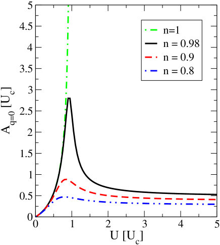
Figure 1: (Color online) The interaction coefficient $A_{q=0}$ for various values of particle density $n$ in units of the Brinkman-Rice critical onsite repulsion$U_{c}$ for a one-dimensional chain.

The double occupancy fluctuations can be expressed in terms of the density fluctuations by use of the antiadiabaticity condition which assumes that the double occupancy adjust to the instantaneous configuration of the chargesei01

$$\frac{\partial E_{e}^{GA,(2)}}{\partial\delta D_{q}}=0$$ (15)

and one obtains the following functional which only depends on the local and intersite charge deviations:

$$E_{e}^{GA,(2)}=\frac{1}{2N}\sum_{q}\left(\begin{array}[]{c}\delta\rho_{q}\\ \delta T_{q}\end{array}\right)\left(\begin{array}[]{cc}A_{q}&B_{q}\\ B^{*}_{q}&C_{q}\\ \end{array}\right)\left(\begin{array}[]{c}\delta\rho_{-q}\\ \delta T_{-q}\end{array}\right)$$ (16)

where

$$\underline{\underline{W_{q}}}^{e-e}=\left(\begin{array}[]{cc}A_{q}&B_{q}\\ B^{*}_{q}&C_{q}\end{array}\right)$$ (19)

is the interaction kernel. The elements of $\underline{\underline{W_{q}}}^{e-e}$ are given by

$$A_{q} = V_{q}-\frac{L_{q}^{2}}{U_{q}}$$ (20)

$$B_{q} = \frac{1}{2}z_{0}\left(z^{\prime}+z_{+-}^{\prime}-z^{\prime}_{D}\frac{2L_{q}}{U_{q}}\right)$$

$$C_{q} = -\ \ 4\frac{(z_{0}z_{D}^{\prime})^{2}}{U_{q}}\cos^{2}(q/2)$$

and the long-wave limit of the $(11)$ element $A_{q=0}$, which dominates the interaction kernel close to half-filling is shown in Fig. 1. For small $U$ one finds $A_{q=0}\approx U/2$ whereas $A_{q=0}$ is enhanced close to the Brinkmann-Rice transition $U=U_{c}$. At exactly half-filling one finds

$$A_{q}=\frac{U(U_{c}+U)(U-2U_{c})}{4U_{c}(U-U_{c})}.$$ (21)

for $U<U_{c}$.

Since the energy expansion in Eq. (16) is a quadratic form in $\delta\rho_{q}$ and $\delta T_{q}$ (see also Eq.(11)), it is useful to introduce the following susceptibility matrix for the non-interacting system $\chi^{0}_{q}$:

$$\underline{\underline{\chi^{0}_{q}(\omega)}}=\frac{1}{N}\sum_{k\sigma}\left(\begin{array}[]{cc}1&-2t\left[\cos(k)+\cos(k+q)\right]\\ -2t\left[\cos(k)+\cos(k+q)\right]&4t^{2}\left[\cos(k)+\cos(k+q)\right]^{2}\end{array}\right)\frac{n_{k+q,\sigma}-n_{k\sigma}}{\omega+\epsilon_{k+q}-\epsilon_{k}-i0^{+}}.$$ (22)

The susceptibility for the interacting system is then obtained from the following RPA series

$$\underline{\underline{\chi_{q}}}=\underline{\underline{\chi_{q}}}^{0}+\underline{\underline{\chi_{q}}}^{0}\underline{\underline{W_{q}}}^{e-e}\underline{\underline{\chi_{q}}}$$ (23)

where the element $(\chi_{q})_{11}$ corresponds to the correlation function for the local charge response.

II.4 Phonon self-energy for the Holstein coupling

As mentioned above, due the local nature of the Holstein coupling Eq. (3) it is not renormalized by the z-factors and thus its quadratic contribution to the energy expansion is given by

$$E_{e-ph}^{hol,(2)}=-\alpha\frac{1}{N}\sum_{q}Q_{-q}\delta\rho_{q}$$ (24)

where $Q_{q}=\sum_{i}\exp(-iqR_{i})u_{i}$ denotes the Fourier transformed (normal) coordinate fluctuation (remember that the saddle-point solution has $u_{i}=u_{0}=0$ so that we can skip the $\delta$ symbol).

Similar we write the lattice energy Eq. (4) as

$$E_{ph}^{hol,(2)}=\frac{1}{2N}\sum_{q}\left\{\frac{P_{q}P_{-q}}{M}+M\Omega^{2}Q_{q}Q_{-q}\right\}$$ (25)

with $\Omega^{2}=K/M$.

The small time dependent deviation from the electronic ground state $\delta\rho_{q}$ will act as a force on the lattice coordinates via $E_{e-ph}^{hol,(2)}$ and the corresponding equation of motion reads

$$M\ddot{Q}_{q}+M\Omega_{q}^{2}Q_{q}=-N\frac{\partial E_{e-ph}^{hol,(2)}}{\partial Q_{-q}}=\alpha\delta\rho_{q}.$$ (26)

As a consequence the lattice vibrations are shifted to new frequencies $\omega_{q}$ which depend on the electronic charge fluctuation $\delta\rho_{q}$

$$\left(\omega_{q}^{2}-\Omega^{2}\right)Q_{q}=-\frac{\alpha}{M}\delta\rho_{q}.$$ (27)

On the other hand $\delta\rho_{q}$ can be determined from linear response theory when we view Eq. (24) as a small perturbation on the electronic system. With the charge susceptibility derived in the previous section one has

$$\delta\rho_{q}=(\chi_{q})_{11}(-\alpha Q_{q})$$ (28)

which upon inserting in Eq. (27) yields

$$\omega_{q}^{2}=\Omega^{2}+\frac{\alpha^{2}}{M}(\chi_{q})_{11}\equiv\Omega^{2}+2\Omega\Sigma_{q}$$ (29)

where $\Sigma_{q}$ denotes the phonon self-energy. In these equations $\chi_{q}(\omega)$ and $\Sigma_{q}(\omega)$ should be evaluated at $\omega=\omega_{q}$. Since the phonon dynamics is assumed to be much slower than the electron dynamics it is a good approximation to evaluate the susceptibilities in the static limit.

We see that in the case of the Holstein coupling the phonon frequency shift is solely determined by the local charge susceptibility renormalized by electronic correlations within the GA. For later use we define the ratio between self-energies in the correlated and uncorrelated case

$$\Gamma_{q}\equiv\frac{\Sigma_{q}(U)}{\Sigma_{q}(U=0)}$$ (30)

which for the Holstein coupling becomes

$$\Gamma_{q}=\frac{(\chi_{q})_{11}}{(\chi^{0}_{q})_{11}}.$$ (31)

In addition it is convenient to introduce the following coupling constant which has energy units

$$g_{hol}=\alpha\sqrt{\frac{1}{2M\Omega}}$$ (32)

so that the phonon self-energy for the Holstein model is given by

$$\Sigma_{q}=g^{2}_{hol}(\chi_{q})_{11}.$$ (33)

II.5 Phonon self-energy for the SSH coupling

The case of the SSH electron-lattice coupling is more subtle since the interaction energy Eq. (9) depends on the z-factors the fluctuations of which we have to consider in the evaluation of $\Sigma_{q}$.

Expansion of Eq. (9) up to second order in the fluctuating fields yields for the Fourier transformed effective electron-lattice interaction

$$E_{e-ph}^{ssh,(2)} = \alpha z_{0}^{2}\frac{1}{N}\sum_{q}\delta T_{q}^{-}Q_{-q}$$

$$+ i\alpha e_{0}z_{0}(z^{\prime}+z_{+-}^{\prime})\frac{1}{N}\sum_{q}\sin(q)\delta\rho_{q}Q_{-q}$$

$$+ 2i\alpha e_{0}z_{0}z_{D}^{\prime}\frac{1}{N}\sum_{q}\sin(q)\delta D_{q}Q_{-q}$$

with the same definitions already introduced in Sec. II.3. Besides the coupling to the transitive fluctuations $\delta T_{q}$ the correlations induce a coupling of the lattice to local density ($\delta\rho_{q}$) and double occupancy ($\delta D_{q}$) fluctuations. Unlike the Holstein case the antiadiabaticity condition now includes the electron-lattice coupling Eq. (II.5) in addition to the bare electronic part Eq. (15),

$$\frac{\partial\left[E_{e}^{GA,(2)}+E_{ph}^{ssh,(2)}\right]}{\partial\delta D_{q}}=0$$ (35)

so that the double occupancy fluctuations can be expressed via the density and lattice fluctuations:

$$\delta D_{q}=2i\alpha z_{0}z_{D}^{\prime}\frac{\sin(q)}{U_{q}}Q_{q}-\frac{L_{q}}{U_{q}}\delta\rho_{q}-\frac{z_{0}z_{D}^{\prime}}{U_{q}}\delta T_{q}.$$ (36)

Inserting Eq. (36) into Eqs. (14,II.5) and including also the (fourier transformed) lattice part Eq. (6) yields

$$E_{tot}^{ssh,(2)}=E_{e}^{GA,(2)}+E_{e-ph}^{ssh,(2)}+E_{ph}^{ssh,(2)}$$ (37)

where $E_{e}^{GA,(2)}$ was derived in Sec.II.3, Eq. (16). The effective coupling of the lattice to the electronic density fluctuations is given by

$$E_{ph}^{ssh,(2)}=\alpha\frac{1}{N}\sum_{q}W^{1}_{q}\delta\rho_{q}Q_{-q}+\alpha\frac{1}{N}\sum_{q}W^{2}_{q}\delta T_{q}Q_{-q}$$ (38)

where we used Eq. (13) to eliminate the antisymmetric fluctuations and introduced the elements of the vector ${\bf W_{q}}^{el-ph}$

$$W_{q}^{1} = ie_{0}z_{0}\sin(q)\left[z^{\prime}+z_{+-}^{\prime}-2z_{D}^{\prime}\frac{L_{q}}{U_{q}}\right]$$

$$W_{q}^{2} = iz_{0}^{2}\tan(q/2)-2ie_{0}(z_{0}z_{D}^{\prime})^{2}\frac{\sin(q)}{U_{q}}.$$

The lattice part becomes

$$E_{ph}^{ssh,(2)}=\frac{1}{2N}\sum_{q}\left\{\frac{P_{q}P_{-q}}{2M}+M\Omega_{q}^{2}Q_{q}Q_{-q}\right\}.$$ (40)

Interestingly the elimination of the double occupancy introduces a novel renormalization of the phonon dispersion

$$\Omega_{q}^{2}=2\frac{K}{M}\left(1-\cos(q)\right)-\frac{1}{M}\left(2\alpha e_{0}z_{0}z_{D}^{\prime}\right)^{2}\frac{\sin^{2}(q)}{U_{q}}.$$ (41)

The (squared) dispersion is composed of the acoustic branch $\sim 1-\cos(q)$ of the uncorrelated atomic chain and a contribution which arises from the double occupancy fluctuations. To the best of our knowledge this is the first time such correlated renormalization of the phonons is reported. We will show below that it induces a phonon softening in addition to the contribution which comes from electronic screening.

The phonon self-energy in the present case can be derived via a similar procedure as before, taking into account the vectorial character of the susceptibility, and reads

$$\Sigma_{q}=g_{q}^{2}\left[{\bf W_{q}}^{el-ph}\right]^{T}\underline{\underline{\chi_{q}}}{\bf W_{q}}^{el-ph}$$ (42)

where the electronic susceptibility matrix $\underline{\underline{\chi_{q}}}$ is obtained from Eq. (23). We also defined the dimensionless coupling constant

$$g_{q} = \sqrt{\frac{\tilde{g}}{\hbar\Omega_{q}}}$$ (43)

$$\tilde{g} = \alpha^{2}\frac{\hbar^{2}}{2M}$$ (44)

In the uncorrelated limit $U=0$ the self-energy reduces to

$$\Sigma_{q}(U=0)=4g_{q}^{2}(U=0)\sin^{2}(q/2)(\chi^{0}_{q})_{22}$$ (45)

where the coupling constant Eq. (43) has to be evaluated with the bare acoustic dispersion $\Omega_{q}^{2}(U=0)=2\frac{K}{M}\left(1-\cos(q)\right)$.

Finally it should be noted that the parameters of the problem are given by $\hbar\omega_{0}\equiv\sqrt{K/M}$, $\tilde{g}$ and $U$ measured in units of the hopping $t\equiv 1$ and we set $\hbar\equiv 1$ in the following.

III Results

III.1 Properties of the TDGA and comparison with exact results

Since in this paper we restrict ourselves to one-dimensional systems it is necessary to analyze the quality of our approximate TDGA scheme in this special limit. With regard to the following investigation of phonon self-energies it is important to figure out which features can be considered as generic and also show up in higher dimensions where our mean-field type approach is expected to perform better.

Since the phonon self-energies are completetly determined by the charge susceptibility (at least in the Holstein case) $(\chi_{q})_{11}$ we first analyze the corresponding TDGA result which for small wave-vectors $q$ and close to half-filling can be expanded as

$$(\chi_{q})_{11}\approx\frac{2}{\pi}\frac{v_{F}q^{2}}{\omega^{2}-(v_{\rho}q)^{2}}$$ (46)

where $v_{F}=v_{F}^{0}z_{o}^{2}$ is the quasiparticle Fermi velocity and $v_{\rho}=v_{F}\sqrt{1+4A_{0}/(\pi v_{F})}$ is the velocity of the (quasi)particle-hole excitations with $A_{0}\equiv A_{q=0}$ defined in Eq. (20). The compressibility $\kappa=-(\chi_{q\to 0})_{11}(\omega=0)$ follows as

$$\kappa=\frac{2v_{F}}{\pi v_{\rho}^{2}}=\frac{2}{\pi}\frac{1}{v_{F}+4A_{0}/\pi}$$ (47)

In the weak coupling limit these expression coincide with the perturbative expressions for the Tomonoga-Luttinger liquid. voit As in the exact case the effective interaction and the Fermi velocity gets renormalized upon increasing $U$.

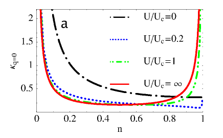
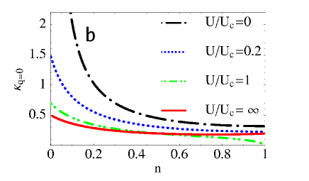
Figure 2: (Color online) 1d-Charge compressibility as a function of $n$ and for different values of $U/U_{c}$ calculated with the Bethe ansatz - exact 1d solution (a) and with the TDGA (b). Here $U_{c}=32t/\pi$ is the Coulomb repulsion at which the Brinkman-Rice transition takes place for $n=1$ in the GA. In the exact solution the metal insulator transition occurs at $U=0$ therefore $U_{c}=32t/\pi$ is used only as an energy unit.

In Fig. 2 we compare the TDGA charge compressibility with the exact 1d solution of the Hubbard model. LW68 ; Shi72 ; Sch90 The renormalization of $v_{F}$ and the effective interaction pushes the qualitative agreement with exact results to larger values of $U$ than the traditional HF+RPA approach. Strong differences arise close to $n=1$. As soon as the interaction is switched on the exact compressibility diverges. This can be understood in the strong coupling limit where the charge degrees of freedom can be mapped to a spinless Fermion modeloga90 and the compressibility is related to the spinless density of states which has a 1d van Hove divergence. In contrast the GA yields a compressibility which tends to zero at the BR point. We remark that the GA compressibility has a jump discontinuity for $n=1$ and $U>U_{c}$. In fact, its left and right limits are finite, while its value computed in $n=1$ is zero. At half-filling an antiferromagnetic (AF) broken symmetry TDGA computation instead of the present paramagnetic one yields much more accurate results. sei01

In the dilute limit the exact compressibility diverges again whereas the TDGA result yields a finite value. This disagreement is not surprising since the RPA in general is well known to fail at low densities. In this case a particle-particle approach, recently implemented on top of the GA, sei07b would be more appropriate.

Despite the (expected) failure of the paramagnetic TDGA at low and half filling at intermediate fillings the behavior of the compressibility as a function of $U$ is qualitative and to some extent quantitatively reproduced. One should keep in mind again that we are using a Fermi liquid approach whereas the real ground state is a Luttinger liquid.

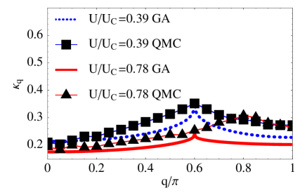
Figure 3: (Color online) 1d-Charge susceptibility ($n=0.6$) as a function of $q/\pi$: comparison between TDGA and QMC results. HS84

In Fig. 3 we compare the TDGA charge susceptibility with QMC results from Hirsch and Scalapino. HS83 ; HS84 Since their data are for $n=0.6$ we expect the TDGA to give reasonable results. Although our formalism is at $T=0$ and the QMC study at $T\neq 0$, the comparison is meaningful because their results are at $T=0.0690$, quite low if compared to the electronic energy scales. The QMC susceptibilities generally agree with ours within ten-twenty percent deviations, and with larger deviations at high $q$ for $U\sim U_{c}$. For large $U$, in fact, the QMC data exhibit the transfer of the peak from $q=2k_{F}$ to $q=4k_{F}$, signature of the spin-charge separation of the 1d-Luttinger liquid, clearly absent in our 1d FL. The QMC curves present a finite $T$ effect that smoothes the peak.

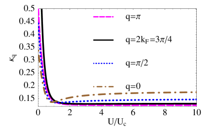
Figure 4: (Color online) 1d-Charge susceptibility as a function of $U/U_{c}$ for $n=0.75$.

The above results indicate that our FL scheme works quantitatively rather well away from half-filling (where an AF TDGA computation would do a better job) and provides reasonable momentum dependencies (but for the subtle Luttinger $4k_{F}$ peak shift for large $U$).

In Fig. 4, we show the charge susceptibility $\kappa_{q}$ as a function of $U/U_{c}$. These results should be taken with a pinch of salt due to the explained drawbacks, however they illustrate well the general behavior of the TDGA that are found in higher dimension where the approach performs better. diciolo08 For small deviations of the density from half-filling the compressibility has a minimum close to $U=U_{c}$ which is due to the corresponding maximum in the $(11)$ element of the interaction kernel (cf. Fig. 1). For large $q$ this minimum becomes too shallow to be clearly seen in Fig. 4. At small momenta the charge susceptibility is close to the compressibility. As the momentum approaches $q=2k_{F}=n\pi$ the charge susceptibility diverges for small $U$. However, this divergence is strongly suppressed upon increasing $U$. At small doping $\kappa_{q}$ is finite but still shows a shallow minimum close to $U=U_{c}$. This behaviour is due to the proximity of the Mott phase which is more clear in higher dimensions. diciolo08 The essential point is that the maximum charge response changes from the wave-vector $q=2k_{F}$ to $q=0$ upon increasing $U$. Therefore correlations suppress the nesting induced transition to a CDW state in favor of phase separation as is discussed in more detailed and higher dimensional systems in Ref. diciolo08, .

It is important to notice that the failures of the TDGA found at high filling in our comparison with the exact results can be traced back to specific features of the 1d physics (like, e.g., the spin-charge separation, the equivalence to spinless fermions at $U=\infty$). Therefore these failures should not be attributed to the TDGA per se, but to the underlying assumption of a FL ground state. This is why our results not only provide qualitative informations on the 1D case, but also shed light on the physics of the FL state occurring at higher dimensions.

III.2 Holstein Coupling

The (static) phonon self-energy for the Holstein coupling $\Sigma^{hol}_{q}\equiv\Sigma_{q}^{hol}(\omega=0)=g_{hol}^{2}[\chi_{q}]_{11}(\omega=0)$ corresponds to the local charge correlation so that the discussion of the previous section directly applies also here. Fig. 5a shows $\Sigma_{q}^{hol}$ for the half-filled system where it is given by

$$\Sigma_{q}^{hol}=g_{hol}^{2}\frac{[\chi^{0}_{q}]_{11}}{1-A_{q}[\chi^{0}_{q}]_{11}}$$

As is clear from the previous section the primary purpose of these results is to illustrate the generic behavior expected in higher dimensions rather than to comprise the physics of 1D systems.

Due to the divergency of $[\chi^{0}_{q}]_{11}$ at $q=2k_{F}=\pi$ the corresponding singularity in $\Sigma_{q}^{hol}$ gets suppressed upon increasing $U$. This suppression persists for all momenta which can also be seen from the vertex $\Gamma_{q}$ (Fig. 5b, cf. Eq. (30) which quantifies the phonon frequency shift for the correlated system as compared to the non-interacting case:

$$\Gamma_{q}=\frac{1}{1-A_{q}[\chi^{0}_{q}]_{11}}.$$ (48)

In the limit $q\to 0$ where $(-\chi^{0}_{q})_{11}$ equals the density of states $N(E_{F})$ the reduction of $\Gamma_{q=0}$ is therefore determined by the effective interaction $A_{q}$ which diverges for $U$ approaching the Brinkmann-Rice transition (and thus $\Gamma_{q}\to 0$). On the other hand, at $q=\pi$ the local non-interacting charge correlations $(\chi^{0}_{q=\pi})_{11}$ display a divergence due to nesting and are thus responsible for the vanishing of $\Gamma_{q\to\pi}$ in this limit.

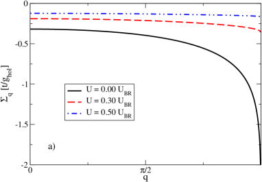
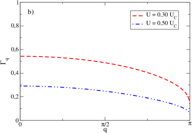
Figure 5: (Color online) a) Self-energy $\Sigma_{q}$ in units of $t/g_{hol}$ and b) ratio between correlated and uncorrelated self-energies $\Gamma_{q}$ for the half-filled Holstein-Hubbard model as a function of momentum $q$.

At finite doping (Fig. 6a) the singularity of $\Sigma_{q}^{hol}$ at $U=0$ occurs at $q=2k_{F}<\pi$ and similar to the half-filled system becomes suppressed upon increasing $U$. As discussed in the previous section (cf. Fig. 4), for large onsite interaction $U$ the charge susceptibility (and thus $\Sigma_{q}^{hol}$) acquires a maximum at small momenta so that the dominant phonon renormalization is shifted from $q=2k_{F}$ to $q=0$. On the other hand (Fig. 6b) the reduction of $\Gamma_{q}$ is still most pronounced at the Fermi momenta $q=2k_{F}$ where the bare Lindhard susceptibility $(\chi^{0}_{q})_{11}$ logarithmically diverges whereas $\Sigma_{q=2k_{F}}(U>0)$ stays finite and thus $\Gamma_{q=2k_{F}}=0$. Of course this is peculiar to the one-dimensional system where one has perfect nesting for each carrier density.

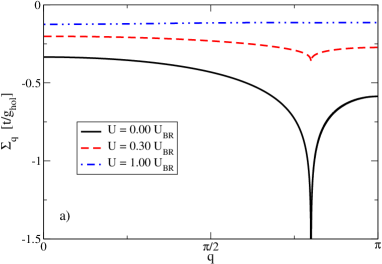
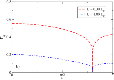
Figure 6: (Color online) a) Self-energy $\Sigma_{q}$ in units of $t/g_{hol}$ and b) ratio between correlated and uncorrelated self-energies $\Gamma_{q}$ for the Holstein-Hubbard model (particle density $n=0.8$) as a function of momentum $q$.

We now analyze in more detail the mode which becomes soft when the dominating instability shifts from $q=2k_{F}$ to $q=0$ for large $U$ and close to half-filling. The dressed phonon propagator

$$D_{q}(\omega)=\frac{D^{0}_{q}(\omega)}{1-g_{hol}^{2}[\chi_{q}]_{11}(\omega)D^{0}_{q}(\omega)}$$ (49)

couples the Holstein phonon $\Omega_{0}$ with the energy of the particle-hole excitations $\sim v_{\rho}q$ when we use the long wavelength limit for the charge susceptibility given in Eq. (46). Then $D_{q}(\omega)$ acquires new poles at

$$\omega^{2}_{+} = \Omega_{0}^{2}+\frac{4g_{hol}^{2}v_{F}}{\pi\Omega_{0}}q^{2}$$ (50)

$$\omega^{2}_{-} = (v_{\rho}q)^{2}-\frac{4g_{hol}^{2}v_{F}}{\pi\Omega_{0}}q^{2}$$ (51)

corresponding to a hardening of the Holstein phonon and a softening of the effective (’zero sound’) particle-hole velocity. Thus the instability at $q=0$ does not follow from a zero in the phonon-type mode but due to the fact that the particle-hole excitation acquire a negative velocity. Since the poles of the dressed charge propagator are identical to those of $D_{q}(\omega)$ this also corresponds to a phase separation instability so that the present approach generalizes the analysis of Ref. Gri94, for $U\to\infty$ Hubbard models to finite onsite interactions.

III.3 SSH coupling

For the transitive electron-phonon coupling we have seen in Sec. II.5 that correlations already induce a renormalization of the phonon dispersion Eq. (41)

$$\Omega_{q}=\sqrt{(\Omega_{q}^{0})^{2}-(\Delta\Omega_{q})^{2}}$$ (52)

due to the elimination of the double occupancy fluctuations (cf. Eqs. (35,36)). Here $\Omega_{q}^{0}=2\omega_{0}\sin(q/2)$ denotes the acoustic branch for $U=0$ and the correlation induced contribution $\sim-(\Delta\Omega_{q})^{2}$ is always negative (since $U_{q}>0$ in Eq. (41)). The corresponding softening of $\Omega_{q}$ is shown in Fig. 7.

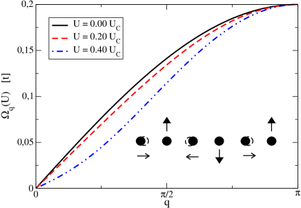
Figure 7: (Color online) Acoustic phonon dispersion in the SSH model for three different $U$ values at half-filling ($\tilde{g}=0.01$, $\omega_{0}=0.1$). Shown is only the influence of the double occupancy fluctuations on $\Omega_{q}$. The inset displays atomic displacements with wave-vector $q=\pi/2$ (horizontal arrows) and the associated modulation of the double occupancy (vertical arrows) with the same periodicity.

The renormalization vanishes for both $q\to 0$ and $q\to\pi$, and is largest for intermediate momenta $q\sim\pi/2$. This can be understood from Eq. (36) where the first term links the displacements to the double occupancy fluctuations $\delta D_{q}\sim\sin(q)/U_{q}Q_{q}$. Remember that $U_{q}$ is the interaction energy of double occupance fluctuations (cf. Eq. (7) which has a significant momentum dependence only close to half-filling and large $U$. Therefore the spatial relation between $Q_{q}$ and $\delta D_{q}$ is mainly determined by $\sin(q)$ and thus largest at $q\approx\pi/2$. The inset to Fig. 7 depicts the corresponding lattice modulation (horizontal arrows) which, due to the inreased (decreased) hybridization, favors a modulation of the density and double occupancies with the same periodicity (vertical arrows).

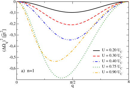
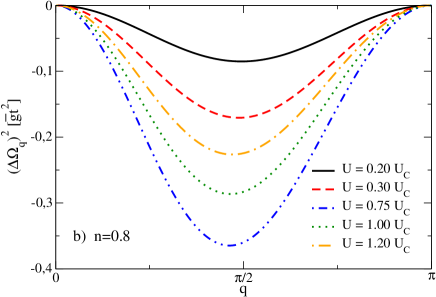
Figure 8: (Color online) Correlation induced correction to the phonon dispersion (in units of $\tilde{g}t^{2}$) from the elimination of double occupancy fluctuations. Charge densities are $n=1$ (panel a) and $n=0.8$ (panel b)

The correction $(\Delta\Omega_{q})^{2}$ to the phonon dispersion induced by the double occupancy fluctuations is separately displayed in Fig. 8. For the half-filled system (top panel) the maximum of $(\Delta\Omega_{q})^{2}$ shifts to smaller $q$-values upon increasing $U$ due to the more significant momentum dependence of $U_{q}$ as mentioned above. This is less pronounced for the doped system (lower panel) where the maximum in the correlation induced correction stays close to $q=\pi/2$. Note also that $(\Delta\Omega_{q})^{2}$ has a maximum as a function of $U$. This is due to the fact that the SSH electron-phonon interaction Eq. (9) is renormalized by the $z$-factors which decrease with increasing $U$ so that the transitive fluctuations become suppressed. In this regard $(\Delta\Omega_{q})^{2}$ results from a subtle interplay of kinetic and correlation effects.

We now turn to the influcence of electronic density fluctuations on the phonon dispersion which is measured in terms of the phonon self-energy $\Sigma_{q}$ Eq. (42).

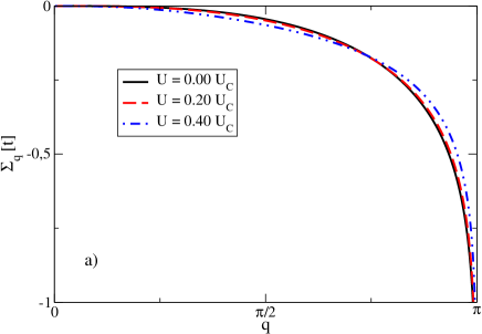
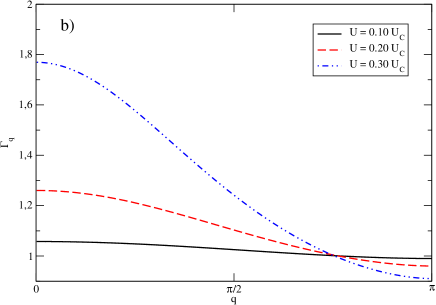
Figure 9: (Color online) a) Phonon self-energy $\Sigma_{q}$ for the half-filled Hubbard-SSH model and different values of $U/U_{c}$. b) Ratio $\Gamma_{q}=\Sigma_{q}(U)/\Sigma_{q}(U=0)$ for the same system. Parameters: $\tilde{g}=0.01$, $\omega_{0}=0.1$.

Fig. 9a displays $\Sigma_{q}$ for the half-filled system. In this limit the local density fluctuations (originating from the Hubbard interaction) are decoupled from the transitive ones. Therefore the latter are not screened and the divergence at $q=\pi$ in case of the SSH coupling is not removed upon increasing $U$ in contrast to the Holstein-Hubbard model. As a consequence, the phonon excitations always (i.e. for infinitesimally small electron-phonon coupling) become instable for $q=\pi$ corresponding to the homogeneous dimerized state. Correlations lead to a suppression (enhancement) of $\Sigma_{q}$ for large (small) momenta as can be more clearly seen from Fig. 9b which shows the ratio $\Gamma_{q}=\Sigma_{q}(U)/\Sigma_{q}(U=0)$. In the limit $q=\pi$ one can show that the ratio is given by $\Gamma_{q=\pi}=z_{0}^{2}$, i.e. it is completely determined by the hopping renormalization factors of the GA. This is consistent with the fact, that for the half-filled dimerized system correlations suppress the dimerization order parameter Hir83 ; baer85 due to the reduction of the effective electron-phonon coupling.

In the limit $q\to 0$ the self-energy vanishes, however, the slope of $\Sigma_{q\to 0}$ strongly depends on the correlations and leads to the observed increase of $\Gamma_{q\to 0}$ with increasing $U$ (Fig. 9b). The main reason for this enhancement comes from the fact that the SSH coupling is a coupling to transitive electronic correlations which at half-filling and small momenta are decoupled from the local ones. In the limit $q\to 0$ and half-filling Eq. (42) becomes

$$\Sigma_{q}^{SSH} \approx g_{q}^{2}|W^{2}_{q}|^{2}(\chi_{q}^{0})_{22}$$ (53)

$$W_{q}^{2} \approx iq\left[z_{0}^{2}+2\frac{U^{2}}{U_{c}^{2}}\right]=iq\left[1+\frac{U^{2}}{U_{c}^{2}}\right]$$ (54)

and one finds that $\Sigma_{q}^{SSH}$ is not screened by the strong local charge fluctuations. On the contrary, since $(\chi_{q}^{0})_{22}\sim 1/z_{0}^{2}$ it becomes enhanced due to the increase of the quasiparticle mass with $U$. However, for the bare SSH coupling $|W^{2}_{q}|^{2}=q^{2}z_{0}^{4}$ this effect would be overcompensated resulting in $\Sigma_{q}\sim z_{0}^{2}$. It is due to the TDGA induced vertex corrections Eq. (54) that the increase of $(\chi_{q}^{0})_{22}$ is even amplified by the concomitant increase of $|W^{2}_{q}|^{2}$ with $U$. Finally, another (though much weaker) factor which leads to the enhancement of $\Sigma_{q\to 0}^{SSH}$ with $U$ comes from the dependence of the coupling constant $g_{q}$ Eq. (43) on the phonon frequencies $g_{q}\sim 1/\sqrt{\Omega_{q}}$ which become softened due to the elimination of the double occupancy fluctuations (cf. Eq. (41)).

The enhancement of the vertex $\Gamma_{q}$ at small momentum is a new effect very much in contrast with the result in the Holstein casediciolo08 where one always finds $\Gamma_{q}<1$, i.e. a reduction of self-energy corrections with $U$.

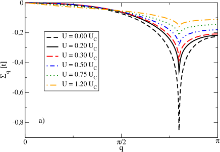
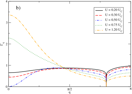
Figure 10: (Color online) a) Phonon self-energy $\Sigma_{q}$ for the doped ($n=0.8$) Hubbard-SSH model and different values of $U/U_{C}$. b) Ratio $\Gamma_{q}=\Sigma_{q}(U)/\Sigma_{q}(U=0)$ for the same system. Parameters: $\tilde{g}=0.01$, $\omega_{0}=0.1$.

Fig. 10 displays the behavior of $\Sigma_{q}$ and $\Gamma_{q}$ for the doped SSH model. Similar to the case of half-filling, $\Sigma_{q}$ is reduced upon increasing $U$ for large momenta. However, the behavior for small $q$ becomes more subtle as can be seen from Fig. 10b. As a function of $U$ the self-energy $\Sigma_{q\to 0}$ passes through a minimum and for large $U$ exceeds again the uncorrelated value (i.e. $\Gamma_{q\to 0}>1$) similar to the half-filled case. This behavior results from a subtle interplay between local and transitive charge fluctuations which are now coupled. For small $U$ the screening induced by the local charge fluctuations leads to a suppression of $(\chi_{q})_{22}$ and also $\Sigma_{q}$. Only at larger $U$ the vertex corrections for $|W^{2}_{q}|$ can overcome this decrease and effectively enhance again the self-energy at small momenta.

The coupling of the local charge density fluctuations also contributes to the suppression of the $q=2k_{F}$ divergence in the self-energy. As in case of the Holstein coupling one therefore finds that $\Gamma_{q=2k_{F}}=0$ since $\Sigma_{q=2k_{F}}(U=0)$ logarithmically diverges whereas $\Sigma_{q=2k_{F}}(U>0)$ stays finite.

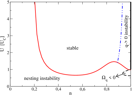
Figure 11: (Color online) Phase diagram for the SSH model with parameters $\tilde{g}=0.02$, $\omega_{0}=0.2$. The solid line indicates the transition to a nesting induced $q=2k_{F}$ instability whereas the dashed-dotted line is the $q=0$ instability line. The region enclosed by the dashed line corresponds to the parameter space where $\Omega_{q}<0$ and the bar at $n=1$ indicates the localized regime for $U>U_{c}$.

Within the Holstein-Hubbard model we have seen that away from half-filling the maximum self-energy shifts from the nesting vector $q=2k_{F}$ to $q=0$ when the correlations become sufficiently strong. As a consequence, a large electron-phonon coupling will induce a CDW instability for small, but a phase separation instability for large $U$, also of course depending on the carrier density. Is there a similar scenario for the transitive coupling in the SSH model? We determine the instabilities from the zero frequency poles of the phonon propagator

$$D_{q}(\omega=0)=\frac{D^{0}_{q}(\omega=0)}{1-\Sigma_{q}D^{0}_{q}(\omega=0)}$$ (55)

which yields the condition

$$\Omega_{q}=-2\Sigma_{q}$$ (56)

and $\Omega_{q}$ is the effective phonon dispersion given in Eq. (41). The solid line in Fig. 11 marks the lattice instability at $q=2k_{F}$, i.e. where the system undergoes a transition towards a combined CDW and bond-order state. This instability is suppressed for large $U$ due to the suppression of the $2k_{F}$ peak in $\Sigma_{q}$ as shown in Fig. 10.

The maximum at $n=0.85$ in the instability line is due the following. At $n=1$ the self-energy can be written as $\Sigma_{q}(U)=z_{0}^{2}\Sigma_{q}(U=0)$ so that upon approaching half-filling the self-energy is determined by both the diverging $\Sigma_{q}(U=0)$ and the Gutzwiller renormalization factor $z_{0}^{2}$ which at $n=1$ tends to zero for $U>U_{c}$ (in Fig. 11 the solid bar at $n=1$ indicates this regime where the charge carriers are localized). As a consequence $|\Sigma_{q}(U)|$ develops a maximum as a function of concentration and fixed $U$ which is reflected in the maximum of the instability line.

Another instability occurs when the system is stable against nesting (i.e. $|\Sigma_{q=2k_{F}}|<\Omega_{q=2k_{F}}/2$) but the slope of $|\Sigma_{q\to 0}|$ becomes larger than the slope of $\Omega_{q\to 0}$. Then there exists another solution of the condition Eq. (56) The transition towards this instability occurs at $q=0$ when both slopes become equal. The corresponding line is shown in Fig. 11) by the dashed dotted curve. Similar to the Holstein-Hubbard model we thus find a $q=0$ instability for large $U$ which here is confined to a region close to half-filling. However, in contrast to the Holstein model, where the phase separation is due to an instability of the ’zero sound’ particle-hole collective mode $v_{\rho}q$ caused by the coupling to the optical phonon we have in the SSH model a coupling between two acoustic modes, i.e. $\Omega_{q}\approx v_{ph}q$ and $v_{\rho}q$. For the situation we have analyzed in Fig. 11 we find always $v_{ph}<v_{\rho}$ so that the mode which becomes unstable has dominantly phonon character. However, since $v_{\rho}$ in the Mott regime is renormalized to very small values one could also imagine a situation where $v_{ph}>v_{\rho}$ in analogy to the Holstein case.

Finally, we have seen that the TDGA applied to the SSH coupling yields an effective phonon dispersion Eq. (41) which yields correlation induced softening through the elimination of double occupancy fluctuations (cf. Fig. 8). For large coupling $\tilde{g}$ these frequencies can become negative even without the consideration of density fluctuations. The corresponding regime in Fig. 11 is enclosed by the dashed line. We find (at least for the present model) that this area is always in a parameter regime which corresponds to the nesting induced instability and therefore never gives rise to a ’real’ instability.

IV Conclusions

We have investigated the renormalization of phonon frequencies within the Hubbard-Holstein and Hubbard-SSH models based on the TDGA approach. Our considerations of the Holstein coupling for one-dimensional correlated systems supplements our investigations in higher dimensions diciolo08 and serves as a reference for our computations of the SSH coupling. In the latter case we have found that correlations influence on the phonon modes $\Omega_{q}$ via two mechanisms. First, the coupling to double occupancy fluctuations leads to a softening which has a maximum around $q=\pi/2$, depending on $U$ and doping. The second mechanism is the standard screening from density fluctuations. However, in this regard our TDGA approach goes beyond the standard RPA since it incorporates the interaction between phonons and both, transitive and induced local density fluctuations. This leads to an interesting dependence of the self-energy $\Sigma_{q}$ on the local repulsion $U$ since it becomes suppressed for large but enhanced for small momenta.

We have found that also the transitive coupling of the Hubbard-SSH model gives rise to an interesting phase diagram where correlations can suppress the $q=2k_{F}$ nesting instability but at the same time are responsible for the occurence of a $q=0$ instability in the vicinity of half-filling. Our calculations therefore indicate that the phase separation instability, previously only evidenced for Holstein-type couplings, seems to be a generic property of strongly correlated electrons coupled to phonons. This is interesting in the context of complex oxides which often show nanoscale phase separation. We have restricted to a short range only model, however the short range phase when supplemented with the long range Coulomb interaction is well known to lead to mesoscopic inhomogeneities. CDCG95 ; lor01I ; lor02 ; low94 ; Ort06 ; Ort07 ; ort08

How do our results apply for higher-dimensional systems, especially with regard to the anomalous softening of bond-stretching modes in perovskite materials? queeney99 ; pintch99 ; Reich96 ; uchiyama04 ; DAs02 ; graf08 Consider e.g. the half-breathing mode in cuprates which involves the movement of two planar oxygen ions towards the central Cu ion. The induced change of the ionic potential on Cu leads to a Holstein-type coupling whereas the associated modulation of the Cu-O hopping integral gives rise to a coupling of the SSH type. Concerning the latter interaction it is interesting that the double occupancy induced renormalization in the 2-D three-band model would lead to a maximum frequency shift at the zone boundary (in contrast to that at $q=\pi/2$ in the 1D SHH model). This kind of interaction therefore induces a downwards dispersion of the half-breathing mode which in the lowest approximation just vibrates at constant frequency. Obviously, in order to account for the doping dependence of the softening one has additionally to consider the effect from the density fluctuations entering the phonon self-energy. In this regard it would be interesting to investigate wether our approach can improve related Hartree-Fock (HF) calculations within the three-band model roesch04 which give an incorrect (i.e. too small) doping dependence of the softening. In fact, since the correlation functions in the TDGA incorporate the correlation induced reduction of the kinetic energy its dependence on the charge carrier concentration is expected to be much more pronounced than in the HF approach. It should be noted that calculations of the density response for the $tJ$-model also indicate a strong renormalization of bond-stretching phonons khali96 with a larger anomaly occuring for half-breathing as compared to full-breathing modes. zhang07

Our theory can be easily extended towards ground states which break translational symmetry. In this regard it would be interesting to evaluate the phonon renormalization from striped ground states since there is experimental evidence Rez06 ; Rez07 that these textures contribute to the anomalous phonon softening at intermediate $q$ values in high-temperature superconductors. Since codoped LSCO compounds, where static stripe order is unambigously established, show a rather strong renormalization it has been argued mukhin07 that the corresponding phonon dispersion exhibits a Kohn-type anomaly originating from the $q=2k_{F}=\pi/2$ scattering along the half-filled stripes. Since the GA (in contrast to HF) leads to half-filled stripes as stable mean-field solutions of the Hubbard model lor02b our approach allows for a test of this scenario from a realistic model.

An interesting issue concerns the question wether the correlation induced enhancement of the phonon self-energy for small wave-vectors in case of the SSH coupling also reflects a corresponding enhancement of the electron-phonon vertex and eventually superconducting correlations. In the present model superconductivity is mediated by the transitive lattice fluctuations which, as we have shown, are not screened in the same way as the local ones and in the long wavelength limit even can be underscreened. This scenario thus appears similar in spirit to previous works by Capone and coworkers cap2001 ; cap2004 where the enhancement of Cooper-pairing near the Mott transition of multiband Hubbard models was investigated. The interorbital fluctuations in these models are only little affected by the correlations (which however lead to a decrease of the quasiparticles bandwidth and a concomitant increase of the density of states near the Fermi level) so that they can effectively enhance superconductivity. An analogous mechanism may also work in the correlated SSH model. However, this issue is much more involved since the investigation of pair-pair scattering requires a GA energy functional which is charge-rotationally invariant sei08 also for the transitive electron-phonon coupling Eq. (9). As a consequence the coupling between pair and lattice fluctuations will in general be different from ${\bf W_{q}}^{el-ph}$ given in Eqs. (II.5,II.5) and will considered elsewhere.

Appendix

In the TDGA expansion Eq.14 we have introduced the following abbreviations for the $z$-factors and its derivatives:

$$z_{i\sigma}\equiv z_{0},\ \ \frac{\partial z_{i\sigma}}{\partial\rho_{ii\sigma}}\equiv z^{{}^{\prime}},$$

$$\frac{\partial z_{i\sigma}}{\partial\rho_{ii-\sigma}}\equiv z^{{}^{\prime}}_{+-},\ \frac{\partial z_{i\sigma}}{\partial D_{i}}\equiv z^{{}^{\prime}}_{D}$$

$$\frac{\partial^{2}z_{i\sigma}}{\partial\rho^{2}_{ii\sigma}}\equiv z^{{}^{\prime\prime}}_{++},\ \frac{\partial^{2}z_{i\sigma}}{\partial\rho_{ii\sigma}\partial\rho_{ii-\sigma}}\equiv z^{{}^{\prime\prime}}_{+-},\ \frac{\partial^{2}z_{i\sigma}}{\partial\rho^{2}_{ii-\sigma}}\equiv z^{{}^{\prime\prime}}_{--}$$

$$\frac{\partial^{2}z_{i\sigma}}{\partial D^{2}_{i}}\equiv z^{{}^{\prime\prime}}_{D},\ \frac{\partial^{2}z_{i\sigma}}{\partial\rho_{ii\sigma}\partial D_{i}}\equiv z^{{}^{\prime\prime}}_{+D},\ \frac{\partial^{2}z_{i\sigma}}{\partial\rho_{ii-\sigma}\partial D_{i}}\equiv z^{{}^{\prime\prime}}_{-D}$$

For the half-filled paramagnetic state we have $z^{{}^{\prime}}=z^{{}^{\prime}}_{+-}$ and $z^{{}^{\prime\prime}}_{+D}=z^{{}^{\prime\prime}}_{-D}$.

References

- (1) S. Maekawa, T. Tohyama, S. E. Barnes, S. Ishihara, W. Koshibae, and G. Khaliullin, Physics of Transition Metal Oxides, Springer (2004).
- (2) R. J. McQueeney, Y. Petrov, T. Egami, M. Yethiraj, G. Shirane, and Y. Endoh, Phys. Rev. Lett. 82, 628 (1999).
- (3) L. Pintschovius and M. Braden, Phys. Rev. B 60, R15039 (1999).
- (4) W. Reichardt, J. Low Temp. Phys. 105, 807 (1996).
- (5) D. Reznik, L. Pintschovius, M. Ito, S. Iikubo, M. Sato, H. Goka, M. Fujita, K. Yamada, G. D. Gu, and J. M. Tranquada, Nature 440, 1170 (2006).
- (6) D. Reznik, T. Fukuda, D. Lamago, A. Q. R. Baron, S. Tsutsui, M. Fujita, and K. Yamada, J. Phys. Chem. Solids 69, 3103 (2008).
- (7) H. Uchiyama, A. Q. R. Baron, S. Tsutsui, Y. Tanaka, W.-Z. Hu, A. Yamamoto, S. Tajima, and Y. Endoh, Phys. Rev. Lett. 92, 197005 (2004).
- (8) M. d’Astuto, P. K. Mang, P. Giura, A. Shukla, P. Ghigna, A. Mirone, M. Braden, M. Greven, M. Krisch, and F. Sette, Phys. Rev. Lett. 88, 167002-1 (2002).
- (9) J. Graf, M. d’Astuto, C. Jozwiak, D. R. Garcia, N. L. Saini, M. Krisch, K. Ikeuchi, A. Q. R. Baron, H. Eisaki, and A. Lanzara, Phys. Rev. Lett. 100, 227002 (2008).
- (10) M. Braden, W. Reichardt, S. Shiryaev, and S. N. Barilo, Physica C 378-381, 89 (2002).
- (11) M. Braden, W. Reichardt, Y. Sidis, Z. Mao, and Y. Maeno, Phys. Rev. B 76, 014505 (2007).
- (12) J. M. Tranquada, K. Nakajima, M. Braden, L. Pintschovius, and R. J. McQueeney, Phys. Rev. Lett. 88, 075505 (2002).
- (13) W. Reichardt and M. Braden, Physica B 263-264, 416 (1999).
- (14) T. Holstein, Ann. Phys. (NY) 8, 325 (1959).
- (15) W. P. Su, J. R. Schrieffer, and A. J. Heeger, Phys. Rev. 22, 2099 (1980).
- (16) W. Kohn, Phys. Rev. Lett. 2, 393 (1959).
- (17) M. Grilli and C. Castellani, Phys. Rev. B 50, 16880 (1994).
- (18) C. Castellani, C. Di Castro, and M. Grilli, Phys. Rev. Lett. 75, 4650 (1995).
- (19) J. E. Hirsch and D. J. Scalapino, Phys. Rev. Lett. 50, 1168 (1983).
- (20) J. E. Hirsch, Phys. Rev. Lett. 51, 296 (1983).
- (21) J. E. Hirsch and D. J. Scalapino, Phys. Rev. B 29, 5554 (1984).
- (22) J. E. Hirsch, Phys. Rev. B 31 6022 (1985).
- (23) E. Berger, P. Valáek, and W. von der Linden, Phys. Rev. B 52, 4806 (1995).
- (24) B. Srinivasan and S. Ramesesha, Phys. Rev. 57, 8927 (1998).
- (25) Z. B. Huang, W. Hanke, E. Arrigoni, and D. J. Scalapino, Phys. Rev. B 68, 220507(R) (2003).
- (26) A. Dobry, A. Greco, J. Lorenzana, and J. Riera, Phys. Rev. B 49, 505 (1994).
- (27) A. Dobry, A. Greco, J. Lorenzana, J. Riera, and H. T. Diep, EPL (Europhysics Letters) 27, 617 (1994).
- (28) J. Lorenzana and A. Dobry, Phys. Rev. B 50, 16094 (1994).
- (29) See e.g. M. Capone, M. Grilli, and W. Stephan, Eur. Phys. J. B11, 551 (1999) and references therein.
- (30) J. K. Freericks and M. Jarrell, Phys. Rev. Lett. 75, 2570 (1995).
- (31) M. Capone, G. Sangiovanni, C. Castellani, C. Di Castro, and M. Grilli, Phys. Rev. Lett. 92, 106401-1 (2004).
- (32) W. Koller, D. Meyer, Y. no, and A. C. Hewson, Europhys. Lett. 66, 559 (2004).
- (33) W. Koller, D. Meyer, and A. C. Hewson, Phys. Rev. B 70, 155103 (2004).
- (34) G. S. Jeon, T. H. Park, J. H. Han, H. C. Lee, and H. Y. Choi, Phys. Rev. B 70, 125114 (2004).
- (35) G. Sangiovanni, M. Capone, C. Castellani, and M. Grilli, Phys. Rev. Lett. 94, 026401 (2005).
- (36) G. Sangiovanni, M. Capone, and C. Castellani, Phys. Rev. B 73, 165123 (2006).
- (37) D. Baeriswyl and K. Maki, Phys. Rev. B 31, 6633 (1985).
- (38) Ju H. Kim and Zlatko Tešanović, Phys. Rev. Lett. 71, 4218 (1993).
- (39) J. Keller, C. E. Leal, and F. Forsthofer, Physica B 206 & 207, 739 (1995).
- (40) M. L. Kuli and R. Zeyher, Phys. Rev. B 49, 4395 (1994); R. Zeyher and M. L. Kuli, Phys. Rev. B 53, 2850 (1996).
- (41) B. J. Alder, K. J. Runge, and R. T. Scalettar, Phys. Rev. Lett. 79, 3022 (1997).
- (42) S. Caprara, M. Avignon, and O. Navarro, Phys. Rev. B 61, 15667 (2000).
- (43) E. Koch and R. Zeyher, Phys. Rev. B 70, 094510 (2004). See also Refs. 18-20 therein.
- (44) E. Cappelluti, B. Cerruti, and L. Pietronero, Phys. Rev. B 69, 161101(R) (2004).
- (45) R. Citro and M. Marinaro, Eur. Phys. J. B 20, 343 (2001).
- (46) R. Citro, S. Cojocaru, and M. Marinaro, Phys. Rev. B 72, 115108 (2005).
- (47) D. Vollhardt, Rev. Mod. Phys. 56, (1984).
- (48) G. Seibold and J. Lorenzana, Phys. Rev. Lett. 86, 2605 (2001).
- (49) G. Seibold, F. Becca, and J. Lorenzana, Phys. Rev. B 67, 085108 (2003).
- (50) G. Seibold, F. Becca, P. Rubin, and J. Lorenzana, Phys. Rev. B 69, 155113 (2004).
- (51) G. Seibold, F. Becca, and J. Lorenzana, Phys. Rev. Lett. 100, 016405 (2008).
- (52) J. Lorenzana and G. Seibold, Phys. Rev. Lett. 89, 136401 (2002).
- (53) J. Lorenzana and G. Seibold, Phys. Rev. Lett. 90, 066404 (2003).
- (54) G. Seibold and J. Lorenzana, Phys. Rev. Lett. 94, 107006 (2005).
- (55) G. Kotliar and A. E. Ruckenstein, Phys. Rev. Lett. 57, 1362 (1986).
- (56) F. Gebhard, Phys. Rev. B 41, 9452 (1990).
- (57) G. D. Mahan, Many-Particle Physics, Plenum Press New York and London (1990).
- (58) J. Voit, Rep. Prog. Phys. 58, 977 (1995).
- (59) E. H. Lieb and F. Y. Wu, Phys. Rev. Lett. 20, 1445 (1968).
- (60) H. Shiba, Phys. Rev. B 6, 930 (1972).
- (61) H. J. Schulz, Phys. Rev. Lett. 64, 2831 (1990).
- (62) M. Ogata and H. Shiba, Physical Review B 41, 2326+ (1990).
- (63) A. Di Ciolo, J. Lorenzana, M. Grilli, and G. Seibold, Phys. Rev. B 79, 085101 (2009).
- (64) O. Rösch and O. Gunnarsson, Phys. Rev. B 70, 224518 (2004).
- (65) S. I. Mukhin, A. Mesaros, J. Zaanen, and F. V. Kusmartsev, Phys. Rev. B 76, 174521 (2007).
- (66) J. Lorenzana, C. Castellani, and C. Di Castro, Phys. Rev. B 64, 235127 (2001).
- (67) J. Lorenzana, C. Castellani, and C. Di Castro, Europhys. Lett. 57, 704 (2002).
- (68) U. Löw, V. J. Emery, K. Fabricius, and S. A. Kivelson, Phys. Rev. Lett. 72, 1918 (1994).
- (69) C. Ortix, J. Lorenzana, and C. Di Castro, Phys. Rev. B 73, 245117 (2006).
- (70) C. Ortix, J. Lorenzana, M. Beccaria, and C. Di Castro, Phys. Rev. B 75, 195107 (2007).
- (71) C. Ortix, J. Lorenzana, and C. Di Castro, Phys. Rev. Lett. 100, 246402 (2008).
- (72) G. Khaliullin and P. Horsch, Phys. Rev. B 54, R9600 (1996); P. Horsch, G. Khaliullin, and V. Oudovenko, Physica C 341-348, 117, (2000).
- (73) P. Zhang, S. G. Louie, and M. L. Cohen, Phys. Rev. Lett. 98, 067005 (2007).
- (74) M. Capone, M. Fabrizio, and E. Tosatti, Phys. Rev. Lett. 86, 5361 (2001).
- (75) M. Capone, M. Fabrizio, C. Castellani, and E. Tosatti, Phys. Rev. Lett. 93, 047001 (2004).
- (76) G. Seibold, F. Becca, and J. Lorenzana, Phys. Rev. B 78, 045114 (2008).