N to $\Delta$ transition form factors with $N_{F}=2+1$ domain wall fermions

Abstract:

The electromagnetic, axial and pseudoscalar nucleon to $\Delta$ form factors are calculated using dynamical domain wall fermions at a lattice spacing of $a=0.114$ fm on a lattice of spatial size $2.74$ fm and pion mass of $331$ MeV. Pion pole dominance and the Goldberger-Treiman relations are examined.

1 Introduction

Form factors measured in electromagnetic and weak processes are fundamental probes of hadron structure. Calculations of such observables using lattice QCD and, in particular, the nucleon form factors [1, 2, 3] has intensified during the last couple of years due to improvements which allow full lattice QCD calculations with controlled lattice systematics [4]. The focus of the current work is the study of the electro-magnetic (EM) and weak N to $\Delta$ transition form factors (FFs). Experiments on the N to $\Delta$ EM transition have yielded accurate results on the EM transition form factor for low momentum transfer [5] that point to deformation of the N/$\Delta$ system. The axial N to $\Delta$ transition FFs are experimentally not well known but there are ongoing experiments using electroproduction of the $\Delta$ resonance to measure the parity violating asymmetry in N to $\Delta$. Lattice QCD enables calculation of these fundamental quantities from first principle. Our previous calculation of these form factors utilized quenched and dynamical Wilson as well as a hybrid scheme with domain wall (DWF) valence quarks on an improved staggered sea [6, 7, 8]. A study of the N to $\Delta$ transition using chiral dynamical quarks in a unitary approach is presented in this work where, in addition, we employ the coherent sink method [2] in order to achieve the better statistical accuracy on the determination of the form factors.

2 Lattice Techniques

We use $N_{F}=2+1$ dynamical domain wall fermions generated by the RBC and UKQCD collaborations [9]. The lattice spacing $a^{-1}=1.73(3)$ GeV is fixed using the $\Omega^{-}$ mass. The length of the fifth dimension is taken sufficiently large to suppress chiral symmetry breaking. Fixing $L_{5}/a=16$ gives an additive residual mass $\sim 10$% of the light quark mass used in this work. We consider configurations on a lattice of size $24^{3}\times 64$ corresponding to pion mass of $0.331(1)$ GeV. We use the standard interpolating operators to create nucleon and $\Delta$ states and employ gauge invariant gaussian smearing of the quark fields with APE-smeared gauge fields optimized for best suppression of excited states for the nucleon [3]. Suppressing excited state contributions in the three-point function is particularly crucial since for this study a source-sink separation of 0.9 fm is used. We show in Fig. 2 that extending the source-sink separation to 1.14 fm the plateau values for the dominant dipole form factor $G_{M1}$, which are the most accurate, are consistent with a time-separation of 0.9 fm, but with a two-fold increase in statistical errors.

The three-point functions that are needed are given by

$$\langle G_{\sigma}^{\Delta J_{\mu}N}(t_{2},t_{1};{\bf p}^{\;\prime},{\bf p};\Gamma_{\tau})\rangle=\sum_{{\bf x}_{2},\;{\bf x}_{1}}e^{-i{\bf p}^{\prime}\cdot{\bf x}_{2}}e^{+i{\bf q}\cdot{\bf x}_{1}}\;\Gamma_{\tau}^{\beta\alpha}\langle\Omega|T\left[\chi_{\Delta}^{\sigma\alpha}({\bf x}_{2},t_{2})J_{\mu}({\bf x}_{1},t_{1})\bar{\chi}_{N}^{\beta}({\bf 0},0)\right]|\Omega\rangle$$ (1)

where $J_{\mu}(x)$ is a local current, ${\bf q}={\bf p}^{\prime}-{\bf p}$ is the momentum transfer, $\sigma$ is the Lorentz vector index for the $\Delta$ and $\Gamma_{\tau}$ projection matrices in Dirac space [7]. The large Euclidean time limit of the ratio

$$R^{J}_{\sigma}(t_{2},t_{1};{\bf p}^{\;\prime},{\bf p}\;;\Gamma_{\tau};\mu)=\frac{\langle G^{\Delta J_{\mu}N}_{\sigma}(t_{2},t_{1};{\bf p}^{\;\prime},{\bf p};\Gamma)\rangle\;}{\langle G^{\Delta\Delta}_{ii}(t_{2},{\bf p}^{\;\prime};\Gamma_{4})\rangle\;}\biggr{[}\frac{\langle G^{\Delta\Delta}_{ii}(t_{2},{\bf p}^{\;\prime};\Gamma_{4})\rangle}{\langle G^{NN}(t_{2},{\bf p};\Gamma_{4})\rangle}\>\frac{\langle G^{NN}(t_{2}-t_{1},{\bf p};\Gamma_{4})\rangle\;\langle G^{\Delta\Delta}_{ii}(t_{1},{\bf p}^{\;\prime};\Gamma_{4})\rangle}{\langle G^{\Delta\Delta}_{ii}(t_{2}-t_{1},{\bf p}^{\;\prime};\Gamma_{4})\rangle\;\langle G^{NN}(t_{1},{\bf p};\Gamma_{4})\rangle}\biggr{]}^{1/2}$$ (2)

yields a time-independent function $\Pi_{\sigma}({\bf p}^{\;\prime},{\bf p}\;;\Gamma_{\tau};\mu)\;$ (plateau region). In addition, all field renormalization constants cancel and therefore $\Pi_{\sigma}$ is a combination of the Lorentz invariant form factors and known kinematical factors. We use sequential inversions through the sink to evaluate the three-point function of Eq. (1). In this method the quantum numbers of the hadron are fixed, which means that a particular value of $\sigma$ and $\Gamma_{\tau}$ must be chosen. This freedom is exploited in the construction of sources for the sequential propagator with the goal to produce optimal linear combinations of $\Pi_{\sigma}$ involving a maximal set of momentum vectors, thereby obtaining a maximum number of statistically independent measurements [6]. It turns out that three such sinks suffice for achieving this goal and enable us to extract the momentum dependence of the electromagnetic, axial and pseudoscalar N to $\Delta$ FFs accurately. A new ingredient of the current work is the use of the coherent sink technique [2] in order to reduce the statistical noise. This consists of creating four sets of forward propagators for each configuration by placing sources at:
$(\vec{0},0),\quad(\vec{L}/2,16),\quad(\vec{0},32)\quad{\rm and}\quad(\vec{L}/2,48).$
From each source $(\vec{x}_{i},T_{i})$, a zero-momentum projected $\Delta$ source is constructed at $T_{0}$ away, i.e. at $(\vec{x}_{i},T_{i}+T_{o})$ and a single coherent backward propagator is calculated in the simultaneous presence of all four sources. The cross terms that arise vanish by gauge invariance when averaged over the ensemble. The forward propagators are already computed by the LHPC Collaboration [2] and therefore we effectively obtain four measurements at the cost of one. This assumes large enough time-separation between the four sources to suppress contamination among them. An open question is whether there exists correlation among these four measurements. In Fig. 2 we show the dependence of the jackknife error on $G_{M1}$ for different coherent sink bin sizes, which verifies that cross-correlations between the different sinks are absent.

The full set of data obtained at a given $Q^{2}$ value is analyzed simultaneously by a global $\chi^{2}$ minimization using the singular value decomposition of an overconstrained linear system [6]. All the results presented here are obtained by analyzing $200$ configurations or a total of $200\times 4=800$ measurements of the ratio given in Eq. (2).

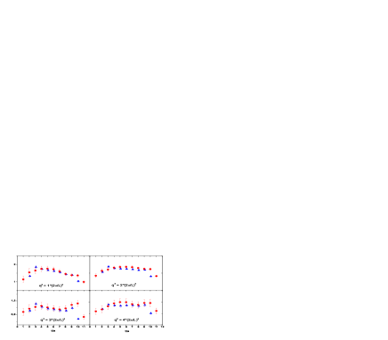
Figure 1: The ratio $S_{1}$ of Eq. (3.2) versus $t/a$ for a source-sink separation 0.91 fm shifted by a time slice (blue triangles) and 1.14 fm (red circles) for the smaller non-zero $\vec{q}^{2}$.

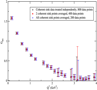
Figure 2: Dependence of the jackknife error for $G_{M1}(Q^{2})$ on the coherent sink bin sizes.

3 Electromagnetic N to $\Delta$ Transition form factors

The electromagnetic transition matrix element is decomposed in terms of three Sachs (FFs)

$$\langle\Delta(p^{\prime},s^{\prime})|j_{\mu}|N(p,s)\rangle=i\,\sqrt{\frac{2}{3}}\;\biggl{(}\frac{m_{\Delta}\;m_{N}}{E_{\Delta}({\bf p}^{\prime})\;E_{N}({\bf p})}\biggr{)}^{1/2}\bar{u}_{\sigma}(p^{\prime},s^{\prime}){\cal{O}}_{\sigma\mu}u(p,s)$$ (3)

with

$${\cal O}_{\sigma\mu}=G_{M1}(q^{2})K_{\sigma\mu}^{M1}+G_{E2}(q^{2})K_{\sigma\mu}^{E2}+G_{C2}(q^{2})K_{\sigma\mu}^{C2}$$

where $K_{\sigma\mu}^{M1},K_{\sigma\mu}^{E2}$ and $K_{\sigma\mu}^{C2}$ are known kinematical factors [7]. In this work we present results for the dominant magnetic dipole form factor $G_{M1}(q^{2})$. Following Ref. [7] we construct the optimized three-point function $S_{1}$ from which $G_{M1}(Q^{2})$ is directly determined

$$S_{1}({\bf q};\mu)=\sum_{\sigma=1}^{3}\Pi_{\sigma}({\bf 0},-{\bf q}\;;\Gamma_{4};\mu)=iA\biggl{\{}(p_{2}-p_{3})\delta_{1,\mu}+(p_{3}-p_{1})\delta_{2,\mu}+(p_{1}-p_{2})\delta_{3,\mu}\biggr{\}}G_{M1}(Q^{2})\quad.$$ (4)

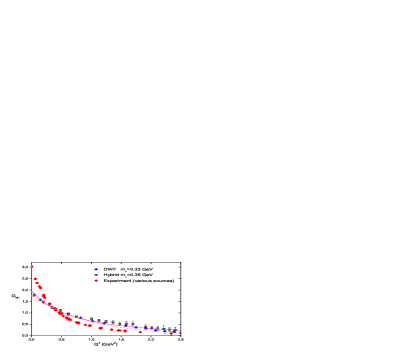
Figure 3: $G_{M1}(Q^{2})$ using DWF fermions and using the hybrid action. The diamonds show experimental results. The solid (dashed) line is a fit to dipole (exponential) form for the DWF data.

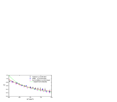
Figure 4: $C_{5}^{A}$ for DWF, the hybrid action and quenched Wilson fermions ( $m_{\pi}$ = 410 MeV) [6]. The green line is a dipole fit to experimental data [10]. The solid (dotted) line is a fit to dipole (exponential) form of the DWF data.

In Fig. 4 we show the results of this work on $G_{M1}(Q^{2})$ using DWF. These are compared with previous results obtained with a hybrid action that uses Asqtad improved staggered fermions generated by the MILC collaboration and domain wall valence quarks [7]. The pion mass in the DWF calculation is 331 MeV and in the hybrid action 350 MeV. These values are close enough to allow a direct comparison. Indeed the results are in very good agreement. Fits to a dipole form, $g_{0}/(1+Q^{2}/m_{0}^{2})^{2}$, as well as to an exponential form $\tilde{g_{0}}\;exp(-Q^{2}/\tilde{m_{0}}^{2})$ described equally well the lattice results. A compilation of the experimentally available data (for more details see Ref. [7]) is also shown in Fig. 4 showing a clear disagreement between lattice results and experiment. This is reflected in the value of the dipole mass of $m_{0}=0.78$ GeV obtained by performing a dipole form fit to the experimental data as compared to $m_{0}=1.164(20)$ GeV for the lattice results. A possible explanation for the faster falloff of the experimental data maybe the lack of significant chiral quark effects –or equally the lack of strong pion cloud– from the still heavy pion mass ensembles that are utilized. Similar behavior is also observed for the nucleon electromagnetic form factors [1], that may again point to the importance of chiral quark effects. The N to $\Delta$ case is particularly clean since there is no ambiguity regarding disconnected contributions and thus the flatter dependence observed in the N to $\Delta$ EM FFs must be of different origin. The large disagreement observed here, however, would require large pion cloud effects to set in as we lower the pion mass. Such large pion effects have been shown to arise in chiral expansions [11] and it is thus interesting to perform the calculation for $m_{\pi}<250$ MeV where they are expected to set in. We are currently analyzing results to extract the subdominant FFs, $G_{E2}$ and $G_{C2}$ using the same DWF configurations.

4 Electroweak N to $\Delta$ Transition form factors and Goldberger-Treiman relations

We consider nucleon to $\Delta$ matrix elements of the axial and pseudoscalar currents defined by

$$A_{\mu}^{a}(x)=\bar{\psi}(x)\gamma_{\mu}\gamma_{5}\frac{\tau^{a}}{2}\psi(x)\hskip 28.45274pt,\hskip 28.45274ptP^{a}(x)=\bar{\psi}(x)\gamma_{5}\frac{\tau^{a}}{2}\psi(x)$$ (5)

where $\tau^{a}$ are the three Pauli-matrices acting in flavor space and $\psi$ the isospin doublet quark field. The invariant proton to $\Delta^{+}$ weak matrix element is expressed in terms of four transition form factors in the Adler representation as

$$<\Delta(p^{\prime},s^{\prime})|A^{3}_{\mu}|N(p,s)> = i\sqrt{\frac{2}{3}}\left(\frac{m_{\Delta}m_{N}}{E_{\Delta}({\bf p}^{\prime})E_{N}({\bf p})}\right)^{1/2}\bar{u}_{\Delta^{+}}^{\lambda}(p^{\prime},s^{\prime})$$ (6)

$$\biggl{[}\left(\frac{C^{A}_{3}(q^{2})}{m_{N}}\gamma^{\nu}+\frac{C^{A}_{4}(q^{2})}{m^{2}_{N}}p{{}^{\prime\nu}}\right)\left(g_{\lambda\mu}g_{\rho\nu}-g_{\lambda\rho}g_{\mu\nu}\right)q^{\rho}+C^{A}_{5}(q^{2})g_{\lambda\mu}+\frac{C^{A}_{6}(q^{2})}{m^{2}_{N}}q_{\lambda}q_{\mu}\biggr{]}u_{P}(p,s).$$

The form factors $C^{A}_{3}(q^{2})$ and $C^{A}_{4}(q^{2})$ belong to the transverse part of the axial current and are both suppressed [8] relative to the dominant form factors $C^{A}_{5}(q^{2})$ and $C^{A}_{6}(q^{2})$. The latter two are the equivalent to the nucleon axial FFs $G_{A}(Q^{2})$ and $G_{p}(Q^{2})$ respectively [6].

The pseudoscalar transition form factor $G_{\pi N\Delta}(q^{2})$, is defined via

$$2m_{q}<\Delta(p^{\prime},s^{\prime})|P^{3}|N(p,s)>=i\sqrt{\frac{2}{3}}\left(\frac{m_{\Delta}m_{N}}{E_{\Delta}({\bf p}^{\prime})E_{N}({\bf p})}\right)^{1/2}\frac{f_{\pi}m_{\pi}^{2}\>G_{\pi N\Delta}(q^{2})}{m_{\pi}^{2}-q^{2}}\bar{u}_{\Delta^{+}}^{\nu}(p^{\prime},s^{\prime})\frac{q_{\nu}}{2m_{N}}u_{P}(p,s)\quad.$$ (7)

Taking matrix elements of the axial Ward-Takahashi identity $\partial^{\mu}A_{\mu}^{a}=2m_{q}P^{a}$ leads to the non-diagonal Goldberger-Treiman (GT) relation

$$C_{5}^{A}(q^{2})+\frac{q^{2}}{m_{N}^{2}}C_{6}^{A}(q^{2})=\frac{1}{2m_{N}}\frac{G_{\pi N\Delta}(q^{2})f_{\pi}m_{\pi}^{2}}{m_{\pi}^{2}-q^{2}}\quad.$$ (8)

The PCAC relation on the hadronic level $\partial^{\mu}A_{\mu}^{a}=f_{\pi}m_{\pi}^{2}\pi^{a},$ relates the pseudoscalar current to the pion field operator and therefore provides the connection to the phenomenological $\pi N\Delta$ strong coupling $g_{\pi N\Delta}=G_{\pi N\Delta}(0)$ that appears in Eq. (8). Assuming pion pole dominance we can relate the form factor $C_{6}^{A}$ to $G_{\pi N\Delta}$ via:

$$\frac{1}{m_{N}}C_{6}^{A}(q^{2}) \sim \frac{1}{2}\frac{G_{\pi N\Delta}(q^{2})f_{\pi}}{m_{\pi}^{2}-q^{2}}$$ (9)

Substituting in Eq. (8) we obtain the simplified Goldberger-Treiman relation

$$G_{\pi N\Delta}(q^{2})\>f_{\pi} = 2m_{N}C_{5}^{A}(q^{2})$$ (10)

in complete analogy to the well known GT relation which holds in the nucleon sector. Pion pole dominance therefore fixes completely the ratio $C_{6}^{A}(q^{2})/C_{5}^{A}(q^{2})$ as a pure monopole term

$$\frac{C_{6}^{A}(q^{2})}{C_{5}^{A}(q^{2})}=\frac{m_{N}^{2}}{m_{\pi}^{2}-q^{2}}\quad.$$ (11)

The goal here is to calculate $C_{5}^{A}(q^{2})$, $C_{6}^{A}(Q^{2})$ and $G_{\pi N\Delta}(Q^{2})$ and check the GT relations using dynamical DWF. The relevant three-point functions required for the calculation of these FFs are obtained at a minimal extra cost using the sequential propagators produced from the optimized nucleon to $\Delta$ source $S_{1}$ and in addition $S_{2}$ which is also used for the electromagnetic transition study of the subdominant FFs. The detailed expressions are given in Ref. [6].

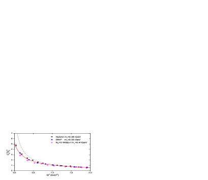
Figure 5: The ratio $C_{6}^{A}/C_{5}^{A}$ versus $Q^{2}$. The dotted line refers to the DWF results and is the pion pole dominance prediction of Eq. (4.5). The solid line is a fit to a monopole form.

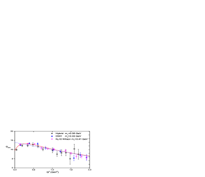
Figure 6: $Q^{2}$-dependence of the pseudoscalar transition form factor $G_{\pi N\Delta}$. The solid line is a fit to pion pole dominance form of Eq. (4.9). The dashed line is a linear fit. The strong coupling constant $g_{\pi N\Delta}$ is the value at $Q^{2}=0$.

In Fig. 4 we compare our results for $C_{5}^{A}$ using DWF to those obtained previously using the hybrid action and quenched Wilson fermions at similar pion masses [6, 8]. The $Q^{2}$ dependence is well described by a dipole Ansatz yielding $C_{5}^{A}(0)=0.970(30)$ and a dipole mass $m_{A}=1.588(67)$ GeV. This is to be compared with the value $m_{A}=1.28\pm 0.10$ GeV extracted by a dipole fit to the available experimental data [10]. As in the case of $G_{M1}(Q^{2})$, we observe a flatter slope for the lattice data, reflected in the larger value of the axial mass $m_{A}$ extracted for the lattice results.

In Fig. 6 we show the ratio $C_{6}^{A}/C_{5}^{A}$. The dotted line shows the pion pole dominance prediction of Eq. (11) where for $m_{N}$ and $m_{\pi}$ we use the lattice values calculated for DWF. The predicted curve does not describe the data at low $Q^{2}$ i.e. in the regime where strong pion cloud effects are expected. Fitting to a monopole form $c_{0}/(Q^{2}/m^{2}+1)$ describes satisfactorily the ratio yielding a heavier mass parameter $m$ than the lattice value of the pion mass. This behavior has been observed also for the other actions [6].

The pseudoscalar form factor $G_{\pi N\Delta}(q^{2})$ is determined optimally from the source $S_{1}$ with a pseudoscalar current operator insertion:

$$S^{P}_{1}({\bf q}\;;\;\gamma_{5})=\sum_{\sigma=1}^{3}\Pi_{\sigma}^{P}({\bf 0},-{\bf q}\;;\Gamma_{4};\gamma_{5})=\sqrt{\frac{2}{3}}\sqrt{\frac{E_{N}+m_{N}}{E_{N}}}\left[\frac{q_{1}+q_{2}+q_{3}}{6m_{N}}\frac{f_{\pi}m_{\pi}^{2}}{2m_{q}(m_{\pi}^{2}+Q^{2})}\right]\;G_{\pi N\Delta}(Q^{2})$$ (12)

We use the value $f_{\pi}=0.1052(7)$ GeV for the pseudoscalar pion decay constant determined in Ref. [9]. The quark mass $m_{q}$ is calculated through the Axial Ward Identity by constructing a suitable ratio of local-smeared and smeared-smeared two-point functions of the axial and pseudoscalar currents [6]. This requires only knowledge of the axial current renormalization $Z_{A}$, which is determined to be $Z_{A}=0.7197(9)$ (Yamazaki et al in [1]), where also $Z_{V}=Z_{A}$ holds up to a small $O(a^{2})$ error for a chiral action [9].

In Fig. 6 we compare results on $G_{\pi N\Delta}(q^{2})$ using dynamical DWF to those obtained with the hybrid action and in the quenched theory [6]. The solid line is a one-parameter fit to the form

$$G_{\pi N\Delta}(Q^{2})=K\>\frac{Q^{2}/m_{\pi}^{2}+1}{(Q^{2}/m_{A}^{2}+1)^{2}(Q^{2}/m^{2}+1)}$$ (13)

expected if the validity of Eq. (11) is assumed. The fit-parameter $K$ provides an estimate of the strong coupling $g_{\pi N\Delta}=G_{\pi N\Delta}(0)=9.6(2)$. A straight line fit of the form $G_{\pi N\Delta}(Q^{2})\sim\biggl{(}1-\Delta\frac{Q^{2}}{m_{\pi}^{2}}\biggr{)}$ as shown by the dashed line, would lead to an estimate $g_{\pi N\Delta}=13.9(6)$. Thus a reliable evaluation of $g_{\pi N\Delta}$ requires further understanding of the behavior at low $Q^{2}$ and in particular of the decrease observed in the hybrid action at $Q^{2}$ close to zero.

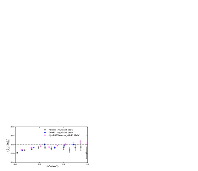
Figure 7: The ratio $f_{\pi}G_{\pi N\Delta}(Q^{2})/m_{N}C_{5}^{A}(Q^{2})$ as a function of $Q^{2}$ relating to the GT validity.

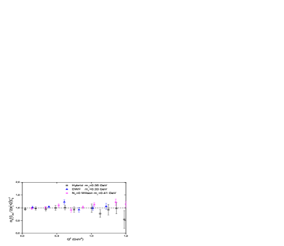
Figure 8: The ratio $m_{N}f_{\pi}G_{\pi N\Delta}(Q^{2})/2(m_{\pi}^{2}+Q^{2})C_{6}^{A}(Q^{2})$ that relates to the validity of Eq. (4.5).

In Fig. 8 we show the ratio $f_{\pi}G_{\pi N\Delta}(Q^{2})/m_{N}C_{5}^{A}(Q^{2})$, which should be unity if the non-diagonal GT relation of Eq. (10) is satisfied. Deviations from this relation are evident in the low $Q^{2}$ regime and they are present for all actions to the same degree which is surprising since one might have expected a better behaviour for DWF. At higher momentum transfers ($Q^{2}>0.5$ GeV²) the relation is satisfied for all actions. On the other hand, the relation given in Eq. (11) that assumes pion pole dominance to relate $C_{6}^{A}$ to $C_{5}^{A}$ is satisfied excellently by the lattice data for all three actions. This agreement is shown in Fig. 8 where the ratio $m_{N}f_{\pi}G_{\pi N\Delta}(Q^{2})/2(m_{\pi}^{2}+Q^{2})C_{6}^{A}(Q^{2})$ is everywhere consistent with unity.

5 Summary and Conclusions

The nucleon to $\Delta$ electromagnetic, axial and pseudoscalar transition form factors are calculated using $N_{f}=2+1$ dynamical domain wall fermions for pion mass of 0.33 GeV. The dominant form factors $G_{M1}$ and $C_{5}^{A}$ show slower falloff with $Q^{2}$ as compared to experiment. A possible explanation maybe that the pion cloud is still not fully developed, at pion mass of 0.33 GeV. We examined the Goldberger-Treiman relations and found that they are satisfied for $Q^{2}>0.5$ GeV² as was previously observed for Wilson fermions and when using a hybrid action. Pion pole dominance relating the axial form factor $C_{6}^{A}$ and the pseudoscalar form factor $G_{\pi N\Delta}$ is satisfied for all values of $Q^{2}$ irrespective of the lattice action used. Extraction of the strong coupling constant $g_{\pi N\Delta}$ requires special care since we need a better understanding of the low $Q^{2}$ behavior of the pseudoscalar matrix element. A calculation on a finer lattice using domain wall fermions is underway to check for any cut-off effects as well as obtain results on the subdominant and phenomenologically interesting electromagnetic quadrupole form factors.

References

- [1] C. Alexandrou et al. [ETMC], arXiv: 0811.0724; C. Alexandrou et al. PoS LAT2009 145 (2009); T. Yamazaki et al., Phys. Rev. D 79 (2009) 114505.
- [2] S. N. Syritsyn et al. (LHPC) arXiv:0907.4194.
- [3] C. Alexandrou, G. Koutsou, J. W. Negele and A. Tsapalis, Phys. Rev. D 74 034508 (2006).
- [4] C. Alexandrou, arXiv:0906.4137 [hep-lat].
- [5] C. Mertz et al. (OOPS), Phys. Rev. Lett. 86, 2963 (2001); K. Joo et al. (CLAS), Phys. Rev. Lett. 88, 122001 (2002); N. F. Sparveris et al., Phys. Rev. Lett. 94, 022003 (2005); S. Stave et al. (OOPS), Eur. Phys. J. A30, 471 (2006), nucl-ex/0604013; N. F. Sparveris et al., Phys. Lett. B651, 102 (2007).
- [6] C. Alexandrou et al., Phys. Rev. D 76 (2007) 094511 ; Erratum to appear.
- [7] C. Alexandrou et al., Phys. Rev. D 77 (2008) 085012 ; C. Alexandrou et al., Phys. Rev. Lett. 94, (2005) 021601.
- [8] C. Alexandrou et al., Phys. Rev. Lett. 98, 052003 (2007);
- [9] C. Allton et al. [RBC-UKQCD Collaboration], Phys. Rev. D 78 (2008) 114509.
- [10] T. Kitagaki et al., Phys. Rev. D 42 (1990) 1331.
- [11] V. Pascalutsa and M. Vanderhaeghen, Phys. Rev. D 73 (2006) 034003.