WUB/09-15

A new model for confinement

Nikos Irges and Francesco Knechtli

Department of Physics, Bergische Universität Wuppertal

Gaussstr. 20, D-42119 Wuppertal, Germany

e-mail: irges, knechtli@physik.uni-wuppertal.de

 

Abstract

We propose a new approach towards the understanding of confinement. Starting from an anisotropic five dimensional pure gauge theory, we approach a second order phase transition where the system reduces dimensionally. Dimensional reduction is realized via localization of the gauge and scalar degrees of freedom on four dimensional branes. The gauge coupling deriving from the brane Wilson loop observable runs like an asymptotically free coupling at short distance, while it exhibits clear signs of string formation at long distance. The regularization used is the lattice. We take the continuum limit by keeping the ratio of the lattice spacing in the brane over the lattice spacing along the extra dimension constant and smaller than one.

 

1 Introduction

Four dimensional $SU(N)$ gauge theories have a unique phase in which interactions are confined [?]. The only known fixed point in their phase diagram which is at vanishing gauge coupling, $g^{2}=0$, is an ultraviolet (UV) fixed point where weak coupling perturbation theory is a good description. According to perturbation theory the interactions in this regime are dominantly of Coulomb type, with the charge obeying the renormalization group (RG) flow appropriate to an asymptotically free coupling[?]. Perturbation theory is however oblivious to the long distance effects of confinement. In order to see those, one must increase the coupling to larger values where the only probe we know of are lattice [?] Monte Carlo (MC) simulations. As the MC simulations reveal, globally the static potential seems to consist of two distinct regimes. At short distance it is indeed of a Coulomb form but at long distance it develops a linearly growing behavior. More precisely, at short distance the coupling $\alpha=g^{2}/4\pi$ defined as (for $SU(2)$)

$$\alpha_{q\bar{q}}(1/r)=-\frac{4}{3}c(r)\,,$$ (1.1)

with $c(r)=(1/2)r^{3}F^{\prime}(r)$ and $F$ the static force, decreases according to the perturbative RG flow and around a certain scale $r_{s}$, defined as the scale where perturbation theory breaks down, $c(r)$ plateaus around the value $-0.3$ [?]. The physically motivated explanation of this behavior comes from an effective string description according to which confinement results in the formation of a string like flux tube. The positive slope of the linear term in the static potential is then interpreted as the tension $\sigma$ of this string. The massless degrees of freedom that describe the fluctuation of the tube are Goldstone modes with an effective action that can be written in the form of a derivative expansion constrained by Poincaré (and perhaps also diffeomorphism) invariance. The kinetic term in this class of ”world-sheet” actions, when integrated out, yields a universal term, the Lüscher term [?], with value $-(d-2)\pi/(24r)$ in $d$-dimensions. This is the term that the MC sees as a plateau in $c(r)$ at large distance. Similar properties are believed to hold for any generalization of the pure gauge theory where the string is stable [?]. In summary, the description of the static potential from short to long distance entails two different analytic methods, namely weak coupling perturbation theory and an effective string description, each of which is blind to the physical effects that the other sees. The two approaches are bridged by the MC which, in principle, can probe the whole static potential from weak to strong coupling. In practice however [?], at short distance, simulations tend to give a much less precise description compared to the usual continuum field theory Feynman diagrams due to the enhanced lattice artifacts and the same applies to any analytic perturbative lattice computation. It is fair to say that a global analytic understanding of the static potential of confined 4d gauge theories is missing.

In [?] we proposed a regularization of four dimensional gauge theories which could allow for such a unified description. The idea is to start form an $SU(N)$ pure gauge theory in 5d and via a systematic expansion around an anisotropic mean-field background [?] try to reach an ultraviolet fixed point (or points) in the interior of the phase diagram where a second order phase transition takes place. The anisotropic background has the value $\overline{v}_{05}$ along the extra dimension and $\overline{v}_{0}$ along the other four directions (see Appendix A). In the confined phase it vanishes while in the deconfined phase it is non-zero along all directions. There is a (unstable according to the leading order mean-field method) phase where $\overline{v}_{0}\neq 0$ and $\overline{v}_{05}=0$, the layered phase. Only on the isotropic lattice the background is isotropic. A line of second order phase transitions was found on the boundary between the deconfined phase and the layered phase. From the side of the deconfined phase, near the phase transition, surprisingly, the system reduces dimensionally. Even though not the same, the physics in this phase is similar in spirit to the layered phase of [?]. We have called in [?] this phase the ”d-compact phase”. The low energy degrees of freedom of the dimensionally reduced system are those of the four dimensional Georgi–Glashow model which is in the class of theories described in the first paragraph. The technical tool used to carry out the expansion is the lattice regularization. This allows for a well defined description and control of the quantum theory but there is a price. Because the final results for the observables are expressed in terms of finite lattice sums it is not easy to take the continuum limit analytically. We emphasize though that this is merely a technical obstruction. The method being fully analytic should, in principle, allow one to carry out all limits without resorting to numerical methods. This will be attempted at a later stage. Here we perform a numerical analysis of the analytic results of [?], with our main focus on the static potential. We will take carefully the continuum limit and we will try to argue that the static potential oriented along the four dimensional hyperplanes, computed in this scheme, reflects both the asymptotically free and the confining aspects of the coupling.

The mean-field expansion comes with certain caveats. The mean-field background is gauge dependent. Within the class of Lorentz gauges we found our physical observables independent of the gauge fixing parameter $\xi$ to leading order [?]. There is no guarantee that the expansion converges. It is known however that the corrections come multiplied by powers of $1/d$ and therefore convergence is expected to become better as the number of dimensions $d$ increases. The mean-field sometimes fakes phase transitions. Even though the known such cases are generally less sophisticated compared to our construction, it is still conceivable that there is an intricate way in which the mean-field does generate a fake picture. This is where the MC investigation of the phase diagram of these theories will be crucial [?]. The reason we proceed with presenting the results of the mean-field ignoring this possibility is that even though the MC may not see an UV fixed point where the system reduces dimensionally, the approach seems to have an independent value. It can serve as a new analytic laboratory of confining gauge theories from short to long distance.

2 The model and its Lines of Constant Physics

The model considered in [?] is an anisotropic $SU(2)$ lattice gauge theory in 5 dimensions defined in a mean-field background. Gauge theories in five dimensions are defined on an anisotropic, infinite, hypercubic lattice via two independent dimensionless parameters. One is $\beta$, the lattice coupling and the other is $\gamma$, the anisotropy parameter. One way to define them is through the dimensionful parameters of the lattice. We consider first finite hypercubic lattices with the same number of lattice points along the four dimensions $L=l/a_{4}$ and along the fifth dimension $L=2\pi R/a_{5}$ and eventually take the $L\to\infty$ limit. $l$ and $R$ are the physical sizes and as appropriate to anisotropic lattices we take different lattice spacings along the four and fifth dimensions. The coupling of a five dimensional gauge theory is denoted by $g_{5}$ and it has dimension of $\sqrt{\rm length}$. The anisotropy parameter can be defined at 0$th$ order as $\gamma=a_{4}/a_{5}=l/(2\pi R)$ and the $SU(2)$ coupling as $\beta=4a_{4}/g_{5}^{2}$. In these variables, the perturbative regime is located at $\beta=\infty$. The above mentioned d-compact phase appears instead for $\beta\sim O(1)$ and $\gamma<1$, obviously far from perturbation theory. The line of second order phase transition extends in a range that corresponds to approximately $\gamma<0.62$. Physically, this is a situation where the extra dimension is larger than the spatial directions and gauge interactions are localized on four dimensional hyperplanes.

The action used to compute observables was the Wilson plaquette action

$$S_{W}=\frac{\beta}{4}\Bigl{[}\frac{1}{\gamma}\sum_{\rm 4d-p}\Bigl{(}1-{\rm tr}\{U_{p}\}\Bigr{)}+{\gamma}\sum_{\rm 5d-p}\Bigl{(}1-{\rm tr}\{U_{p}\}\Bigr{)}\Bigr{]},$$ (2.2)

where the first term contains the effect of all plaquettes $U_{p}$ along the four dimensional slices of the five dimensional space and the second term contains the effect of plaquettes having two of their sides along the extra dimension. In the mean-field, for $SU(2)$, the fluctuating degrees of freedom are complex valued quantities $V(n,M)$ located at the lattice site $n$ and pointing in the direction $M$. The schematic expression for the correction to the expectation value of a physical, gauge invariant observable ${\cal O}$ to second order in the mean-field expansion has the form

$$<{\cal O}> = {\cal O}[\overline{V}]+\frac{1}{2}\left(\frac{\delta^{2}{\cal O}}{\delta V^{2}}\right)_{ik}\left(K^{-1}\right)_{ik}$$

$$+ \frac{1}{24}\sum_{i,k,l,m}\left(\frac{\delta^{4}{\cal O}}{\delta V^{4}}\right)_{iklm}\Bigl{(}(K^{-1})_{ik}(K^{-1})_{lm}+(K^{-1})_{il}(K^{-1})_{km}+(K^{-1})_{im}(K^{-1})_{kl}\Bigr{)}$$

where $K$ is the appropriate lattice propagator and the sums over $i,k,l,m$ are sums over links. Derivatives and contractions are taken in the mean-field background. All such quantities are gauge independent. Polyakov loops with scalar and vector transformation properties represent corresponding classes of states in the Hilbert space and from the exponential decay of their Euclidean time correlators their mass spectra can be extracted. The expectation value of Wilson loops can be used to extract the static potential. The anisotropic lattice admits two inequivalent classes of Wilson loops. One class consists of the loops oriented along the time direction and one of the spatial directions. The other class consists of loops along the time and the extra dimension, the latter defined as the direction along which the background is different from the background along the other four directions. We call the static potentials derived from these two classes as $V_{4}$ and $V_{5}$ respectively and define as $F_{j}(r-a_{j}/2)=\{V_{j}(r)-V_{j}(r-a_{j})\}/a_{j}$, $j=4,5$ the corresponding forces.

The dimensionless vector mass (see Eq. (A.47)) is found to have a dependence only on the lattice size[?]

$$a_{4}m_{W}=c_{L}/L\,,$$ (2.4)

where $c_{L}$ is a constant with numerical value $12.61$. Therefore the system can not be in the Higgs phase in a mean-field background. Hence, if dimensionally reduced, it must be in a confined phase. The scalar mass $a_{4}m_{H}$ (see Eq. (A.44)) can be used to measure a critical exponent of $\nu=1/2$ as the second order phase transition is approached. The potential $V_{5}(r)$ (see Eq. (A)) determines the interaction of static quarks along the extra dimension. The static potential $V_{4}(r)$ (see Eq. (A.41)) is the quantity that dictates the behavior of the dimensionally reduced coupling and it is well defined for any value of the distance $r$. For more details on these computations we refer the reader to [?].

It is convenient to trade the bare lattice coupling $\beta$ for the dimensionless physical ratio $\rho=a_{4}m_{W}/a_{4}m_{H}$ and parametrize the model by the two dimensionless physical ratios $\rho$ and $\gamma$. The lattice spacing can be then chosen to be measured by $a_{4}m_{H}$. An issue arises when one realizes that on an infinite lattice both the numerator and the denominator of $\rho$ approach zero in the limit $a_{4}\to 0$. This means that the continuum limit must be reached in a way that regularizes $\rho$. The method to achieve this is to approach the phase transition at fixed $\gamma$ and at every step, adjust $L$ and $\beta$ so that $\rho$ remains constant. When taken in this way, the infinite lattice and continuum limits coincide:

$$(L\longrightarrow\infty,\;\;\beta\longrightarrow\beta_{c})|_{\gamma,\rho={\rm const}}\;\;\Longleftrightarrow\;\;{\rm continuum\;limit}$$ (2.5)

A crucial fact that allows one to apply this method without obstacles is the fact that $a_{4}m_{W}$ depends only on $L$ and that $a_{4}m_{H}$ depends only on $\beta$ and $\gamma$. We call from now on such continuum limit trajectories on the phase diagram approaching the phase transition Lines of Constant Physics (LCPs). The whole discussion above can be generalized to any $SU(N)$ gauge group. Here we concentrate only on $SU(2)$.

3 The continuum limit

Following [?] we define a physical scale through the condition

$$r_{\rm s}^{2}F_{4}(r_{\rm s})=s=0.2\,.$$ (3.6)

$s=0.2$ is chosen so that $r_{s}/a_{4}$ lies in the transition region from the short distance behavior of the force to the long distance one.

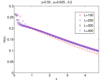
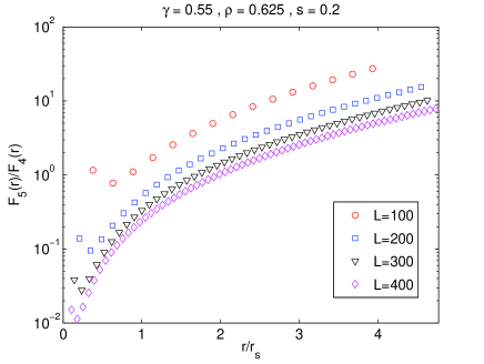
Figure 1: Left Plot: the function $H(x)$ in Eq. (3.8) along the LCP A. Right plot: the ratio of the extra dimensional to four dimensional force $F_{5}(r)/F_{4}(r)$ along the LCP A.

We will first consider the LCP trajectory defined as

$${\rm LCP\;A}:\;\;\;\gamma=0.55\;\;{\rm and}\;\;\rho=0.625\,,$$ (3.7)

then consider other values of $\rho$ for the same $\gamma$ and finally we will analyze other LCPs labelled by values in the range $0.62>\gamma>0$ (i.e. move down along the line of second order phase transitions).

In the left plot of Fig. 1 we show the dimensionless function

$$H(x)=\left.F_{4}(r)r^{2}\right|_{r=xr_{s}}$$ (3.8)

for various lattice spacings corresponding to $L$ values in the range $100,\ldots,400$. The function shows good scaling. The shape of $H(x)$ is different than in a pure $SU(2)$ gauge theory, see [?], in particular it decreases as $x$ increases. We will see below that this is due to the presence of a positive $1/r^{2}$ contribution at short disctance and a large negative logarithmic contribution at large distance in the static potential $V_{4}$.

In the right plot of Fig. 1 we show the ratio $F_{5}(r)/F_{4}(r)$ on a logarithmic scale as a function of $r/r_{s}$ for different lattices along the LCP A. When we take the continuum limit the ratio decreases steadily which implies that the force $F_{5}$ is not physical. This is an evidence for localization: since $F_{4}$ has a finite continuum limit (see left plot in Fig. 1), $F_{5}$ tends to zero, implying that the five dimensional space decomposes into a set of non-interacting Euclidean four-branes along the fifth dimension. On each of these branes the localized light degrees of freedom are therefore expected to be those of the four dimensional Georgi–Glashow model. Since the mean-field background does not break the gauge symmetry spontaneously, these degrees of freedom must be in the confined phase. In the following, we will take the continuum limit of the static potential $V_{4}$ and try to argue that our picture of dimensional reduction is consistent.

To extract physical information from the static potential Eq. (A.41) we start from an ansatz of the form

$$V(r)=\mu+\sum_{p}\frac{c_{p}}{r^{p}}\,,$$ (3.9)

with $p\geq-1$ ($p=0$ corresponds to a logarithmic term and $c_{-1}\equiv\sigma$), solve locally for the coefficients $c_{p}$ and plot them as a function of $r$ (in practice we will rescale all dimensionful quantities by appropriate powers of $r_{s}$ to make them dimensionless). The limit $L\to\infty$ will be taken by computing the coefficients for increasing values of $L$ and extrapolating to the infinite lattice.

3.1 Short distance

For $r/r_{s}<1$ we choose the ansatz

$$V(r)=\mu+\frac{c_{1}}{r}+\frac{c_{2}}{r^{2}}\,,$$ (3.10)

the role of the $1/r^{2}$ term being the check of an imperfect dimensional reduction.

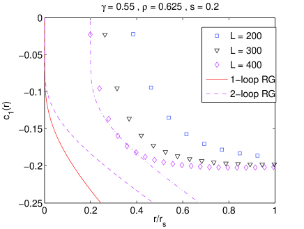
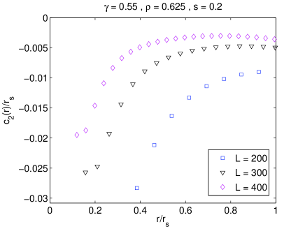
Figure 2: The short distance coefficients $c_{p}$ for the LCP A.

In Fig. 2 we compute $c_{1}$ and $c_{2}$ (see Appendix B) and compare the coefficient $c_{1}$ to the 1-loop and 2-loop RG evolution formula

$$\Lambda_{q\bar{q}}\,r=\left(b_{0}g^{2}\right)^{-b_{1}/(2b_{0}^{2})}e^{-1/(2b_{0}g^{2})}\,,$$ (3.11)

where $g^{2}=-(16\pi/3)\,c_{1}$ and $g^{2}=g^{2}(1/r)$. For the Georgi–Glashow model $b_{0}=7/(4\pi)^{2}$ and $b_{1}=(115/3)/(4\pi)^{4}$. The 1-loop formula is obtained for $b_{1}=0$. Unlike for QCD there is no available experimental or lattice MC prediction for a scale, so we will choose it according to convenience to $\Lambda_{q\bar{q}}\,r_{s}=0.277$. Also, due to the high degree of the discrete derivatives involved in the determination of $c_{1}(r)$, the latter can be defined only for $r/a_{4}>2$ which makes the comparison with the RG formula valid near $r=0$ hard. Nevertheless, it is clear from the left of Fig. 2 that even though the continuum limit has not been reached, as $L$ increases there is a stable convergence to the theoretical curve. The continuous line on the left is the 1-loop curve and the dashed one on the right is the 2-loop curve. To illustrate our point we have shifted the 2-loop curve by a constant, shown as a dashed dotted line. In addition, according to the right of Fig. 2, as $L\to\infty$, the $1/r^{2}$ piece gradually disappears.

3.2 Long distance

For $r/r_{s}>1$ we choose the ansatz

$$V(r)=\mu+\sigma r+c_{0}\log(r)+\frac{c_{1}}{r}+\frac{c_{2}}{r^{2}}$$ (3.12)

and compute the coefficients using the discretized formulae in Appendix B. The plots show plateaus forming for all four coefficients at the same range of distances

$$r/r_{s}\in[2.15\,,\,2.80],$$ (3.13)

a sign that the ansatz is close to the actual form. Moreover we have checked that the plateaus form essentially independently from the way we discretize the derivatives of $V(r)$. We take as the plateau value of a coefficient the average of the quantity over the range indicated in Eq. (3.13). Reading off the value of a coefficient (or of a mass) from a plateau introduces errors, which we add on its plot. In Fig. 3 we compute the continuum limit of the $c_{p}$ for the LCP A using a linear fit in $a_{4}^{2}$, which is the expected form of leading cut-off effects in the static potential [?].

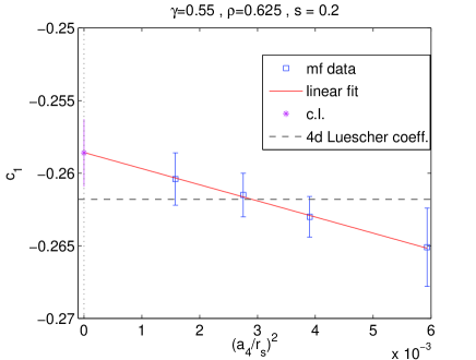
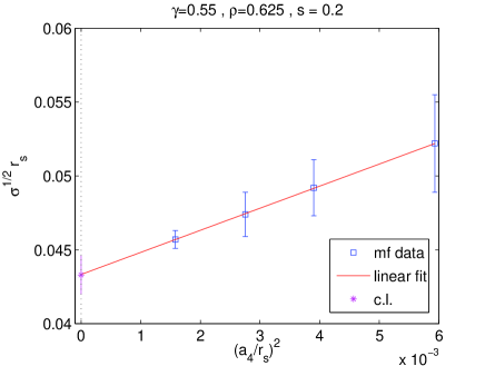
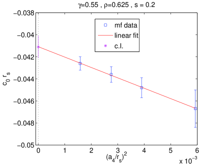
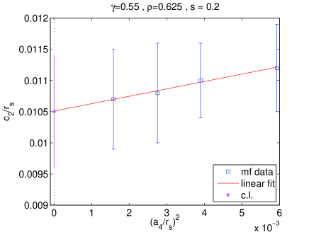
Figure 3: The continuum limits of the long distance coefficients $c_{p}$ for the LCP A.

The continuum limit value of the string tension is

$$\sqrt{\sigma}\,r_{s}=0.0433(13)$$ (3.14)

and using the scale $\Lambda_{q\bar{q}}$ estimated in Section 3.1 we obtain roughly $\Lambda_{q\bar{q}}/\sqrt{\sigma}\simeq 6.4$. Even though not from the same theory, the pure four dimensional $SU(2)$ gauge theory value [?,?] (which is the only quantitatively reliable case we know) $\Lambda_{q{\bar{q}}}^{({\rm YM})}/\sqrt{\sigma}\simeq 0.68(10)$ tells us that the string tension is probably rather small in our model. A physical understanding of this fact can be obtained by reading off the continuum limit value

$$\sqrt{\sigma}\,l=0.69$$ (3.15)

from Fig. 3 and Fig. 4: the box seems to be barely sufficiently large to sustain a stable string. In order to increase this number, one would need to increase $l$, which as we will argue in the following, requires decreasing $\rho$ and increasing $L$. On the other hand, the continuum limit value of the coefficient $c_{1}$ is

$$c_{1}=-0.2586(23)\,,$$ (3.16)

in excellent agreement with the universal value of the $d=4$ Lüscher coefficient $-\pi/12$, as it should. The somewhat surprising term that seems to be though necessary for a correct interpretation of our formulae is the $\log(r)$ term. In fact, if left out, a consistent picture can be hardly obtained. Regarding the $1/r^{2}$ term that we seem to be also seeing, as well as other possible higher negative powers of $r$ we would not like to make any committing statements until a more complete understanding of the structure of the lattice formula Eq. (A.41) both from the field theory and the effective string point of view is obtained.

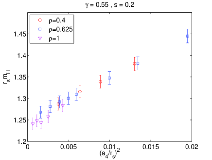
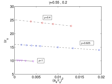
Figure 4: The continuum limits of $r_{s}m_{H}$ and $l/r_{s}$. The errors of $m_{H}$ originate from the ones of $m_{W}$ and come from the uncertainty in the effective mass at $L=100$. $m_{W}$ is scaled proportional to $1/L$. On the right linear fits in $a_{4}^{2}$ show the continuum limit.

The next issue concerns the universality of the continuum limit. It is easier to formulate the question in physical terms. In Fig. 4 we compute the continuum limits of $r_{s}m_{H}$ (left) and of $l/r_{s}$ (right) for three RG trajectories at $\gamma=0.55$ with different $\rho$ values of $0.4$, $0.625$ and $1$. Evidently, $r_{s}m_{H}$ has (within errors) a $\rho$ independent continuum limt, around $1.25$. $\rho$ on the other hand, when $L$ is varied, controls the physical size of the lattice, i.e. the size of the box: as $\rho$ increases, the box shrinks. When $L$ is kept constant, it controls the lattice spacing: as $\rho$ increases, the lattice spacing decreases. It is interesting to notice that since $\rho\,(l/r_{s})$ has a universal continuum limit which is around $10$, and because (by definition) $\rho\,(l/r_{s})\,(r_{s}m_{H})=c_{L}$, the continuum limit value of $c_{L}$ is, within its error, the same as its finite $L$ value $12.61$. Finally the critical law of approach to the phase transition along an LCP can be expressed as [?]

$$\beta=\beta_{c}\,\frac{1}{1-k\,\left(\frac{\displaystyle c_{L}}{\displaystyle\rho\,L}\right)^{2}}\,,$$ (3.17)

with $k$ some constant, confirming that it is indeed the quantity $\rho\,L$ which controls the limit.

To approach the continuum limit at a given value of $\gamma$ (at a sufficiently large $L$) it is convenient to first tune $\rho$ to an optimal value and then take $L$ as large as possible, the latter being the more time consuming step. The larger $\gamma$ is, that is the more isotropic the box becomes, the smaller box is appropriate to sustain a string (in a large box a small anisotropy is nearly unnoticeable), which means that a larger $\rho$ will be needed. But the box can not be arbitrarily small. The string being a long distance effect, will be unstable in a too small box. Thus, we expect to have an upper limit on $\rho$

$$\rho<\rho_{\rm inst}\qquad\mbox{(at given $L$)}\,,$$ (3.18)

beyond which some sign of instability should appear. Indeed, beyond a certain $\rho$ the string tension turns negative, a typical sign of instability. On the other hand when $\gamma$ is small, the physical volume of the four dimensional branes shrinks compared to the extra dimension and therefore a large box, i.e. a small $\rho$ is necessary to sustain a string. But the box can not be arbitrarily large either. A lower bound

$$\rho>\rho_{\rm dr}\qquad\mbox{(at given $L$)}$$ (3.19)

on the possible values of $\rho$ exists, beyond which the critical law Eq. (3.17) is not valid anymore and dimensional reduction is lost. The coefficients $\sigma$, $c_{0}$, $c_{1}$ plateau at zero with only $c_{2}$ remaining non-trivial, as appropriate to a five dimensional static potential. Also the ratio $F_{5}/F_{4}$ approaches a constant, which is 1 for the isotropic case.

The above discussion implies essentially that only a box whose physical size and anisotropy are within a certain allowed (correlated) range can describe a continuum four dimensional theory with a stable string. It turns out that in our case this range for the anisotropy parameter is around

$$0.6>\gamma>0.5\,,$$ (3.20)

a rather narrow window. Our prime example, LCP A (for which $\gamma=0.55$), falls in the middle of this range. As either of the two bounds in Eq. (3.20) is approached the system seems to require very quickly huge lattices in order that the continuum limit is reached. For $\gamma=0.55$ the physical size of the lattice can be approximately in the range $2>\rho>0.5$. Outside this range we observe either a negative string tension or five dimensional physics. Again, soon deviating from the LCP A value ($\rho=0.625$), the continuum limit seems to demand larger lattices than we can afford at the moment.

The remaining question is how to construct such a box that fits the “universe”. The answer is in Fig. 4 and Eq. (3.17): we start with values $\rho_{1}$ and $L_{1}$ that describe four dimensional physics (for LCP A this is realized at $\rho_{1}=0.625$ and $L_{1}=400$) and decrease $\rho_{2}<\rho_{1}$ adjusting the lattice size so that $L_{2}\geq(\rho_{1}/\rho_{2})L_{1}$. Like this $\beta$ in Eq. (3.17) does not increase and the bound Eq. (3.19) is not violated. In particular these operations should make it possible to eventually reach $\sqrt{\sigma}\,l>1$. Finally, it is interesting to observe that in this limit the scalar mass becomes much larger than the vector mass.

4 Conclusions

A five dimensional pure gauge theory on an anisotropic lattice can be described by fluctuations around a mean-field background. The phase diagram has a line of ultraviolet fixed points where the system can reduce to a collection of non-interacting Euclidean four-branes and the continuum limit can be taken. The static potential together with the masses of the lightest fields can be used to describe the system away from perturbation theory. The four dimensional gauge coupling derived from the static potential at short distance runs like an asymptotically free coupling while at long distance it becomes the Lüscher coefficient of a confining string. The four dimensional theory recovered in the continuum limit is not a pure $SU(2)$ gauge theory. The potential shows confinement but also has a large logarithmic contribution and the vector particle is lighter than the scalar. This theory should correspond to a region in the parameter space of the Georgi–Glashow model.

Even though we have computed all the observables analytically, we did the continuum limit analysis numerically. Clearly, the success with which the model passed several severe tests calls for further study, where the lattice propagator is inverted analytically and the finite lattice sums are performed explicitly. Then the continuum limit itself could be studied analytically.

The static potential is computed using a MATLAB code. Using an AMD Phenom II 3.2 GHz processor, the computational cost is 35 core-hours on a $L=200$ lattice and about $34$ core-days on a $L=400$ lattice.

Acknowledgments. We thank R. Sommer for correspondence. N. I. acknowledges the support of the Alexander von Humboldt Foundation via a Fellowship for Experienced Researcher.

Appendix A Appendix

In this Appendix we summarize the expressions for the observables computed analytically in [?] and analyzed numerically here in the main text.

The propagator in momentum space is defined as

$${\tilde{K}}=-{{\tilde{K}}^{(hh)-1}}+{\tilde{K}}^{(vv)}$$ (A.21)

with

$${\tilde{K}}^{(hh)}=-\delta_{p^{\prime}p^{\prime\prime}}\delta_{\alpha^{\prime}\alpha^{\prime\prime}}\frac{I_{2}({\overline{h}}_{0})}{{\overline{h}}_{0}I_{1}({\overline{h}}_{0})}\left[1-\epsilon\cdot\frac{{\overline{h}}_{0}}{I_{2}({\overline{h}}_{0})}\left(\frac{I_{2}^{2}({\overline{h}}_{0})}{I_{1}({\overline{h}}_{0})}-I_{3}({\overline{h}}_{0})\right)\right]\cdot{\rm diag}(1,1,1,1,0)$$

$$-\delta_{p^{\prime}p^{\prime\prime}}\delta_{\alpha^{\prime}\alpha^{\prime\prime}}\frac{I_{2}({\overline{h}}_{05})}{{\overline{h}}_{05}I_{1}({\overline{h}}_{05})}\left[1-\epsilon\cdot\frac{{\overline{h}}_{05}}{I_{2}({\overline{h}}_{05})}\left(\frac{I_{2}^{2}({\overline{h}}_{05})}{I_{1}({\overline{h}}_{05})}-I_{3}({\overline{h}}_{05})\right)\right]\cdot{\rm diag}(0,0,0,0,1)$$ (A.22)

where $\epsilon=1$ for $\alpha^{\prime}=0$ and $\epsilon=0$ for $\alpha^{\prime}\neq 0$,

$${\tilde{K}}^{(vv)}_{\alpha^{\prime}\neq 0}=\delta_{p^{\prime}p^{\prime\prime}}\delta_{\alpha^{\prime}\alpha^{\prime\prime}}(-2\frac{\beta}{\gamma}{\overline{v}}_{0}^{2})\cdot$$

$$\left(\begin{array}[]{cc}\sum^{\prime}c_{M^{\prime}}-\frac{1}{\xi}s^{2}_{0/2}\hskip 28.45274pt2s_{0/2}s_{1/2}\hskip 28.45274pt2s_{0/2}s_{2/2}\hskip 28.45274pt2s_{0/2}s_{3/2}\hskip 28.45274pt2s_{0/2}s_{5/2}\gamma^{2}\frac{\overline{v}_{05}}{{\overline{v}}_{0}}\\ 2s_{1/2}s_{0/2}\hskip 28.45274pt\sum^{\prime}c_{M^{\prime}}-\frac{1}{\xi}s^{2}_{1/2}\hskip 28.45274pt2s_{1/2}s_{2/2}\hskip 28.45274pt2s_{1/2}s_{3/2}\hskip 28.45274pt2s_{1/2}s_{5/2}\gamma^{2}\frac{\overline{v}_{05}}{{\overline{v}}_{0}}\\ 2s_{2/2}s_{0/2}\hskip 28.45274pt2s_{2/2}s_{1/2}\hskip 28.45274pt\sum^{\prime}c_{M^{\prime}}-\frac{1}{\xi}s^{2}_{2/2}\hskip 28.45274pt2s_{2/2}s_{3/2}\hskip 28.45274pt2s_{2/2}s_{5/2}\gamma^{2}\frac{\overline{v}_{05}}{{\overline{v}}_{0}}\\ 2s_{3/2}s_{0/2}\hskip 28.45274pt2s_{3/2}s_{1/2}\hskip 28.45274pt2s_{3/2}s_{2/2}\hskip 28.45274pt\sum^{\prime}c_{M^{\prime}}-\frac{1}{\xi}s^{2}_{3/2}\hskip 28.45274pt2s_{3/2}s_{5/2}\gamma^{2}\frac{\overline{v}_{05}}{{\overline{v}}_{0}}\\ 2s_{5/2}s_{0/2}\gamma^{2}\frac{\overline{v}_{05}}{{\overline{v}}_{0}}\hskip 14.22636pt2s_{5/2}s_{1/2}\gamma^{2}\frac{\overline{v}_{05}}{{\overline{v}}_{0}}\hskip 14.22636pt2s_{5/2}s_{2/2}\gamma^{2}\frac{\overline{v}_{05}}{{\overline{v}}_{0}}\hskip 14.22636pt2s_{5/2}s_{3/2}\gamma^{2}\frac{\overline{v}_{05}}{{\overline{v}}_{0}}\hskip 14.22636pt\gamma^{2}\left(\sum^{\prime}c_{M^{\prime}}-\frac{1}{\xi}s^{2}_{5/2}\right)\\ \end{array}\right)$$ (A.28)

(A.29)

and

$${\tilde{K}}^{(vv)}_{\alpha^{\prime}=0}=\delta_{p^{\prime}p^{\prime\prime}}\delta_{\alpha^{\prime}\alpha^{\prime\prime}}(-2\frac{\beta}{\gamma}{\overline{v}}_{0}^{2})\cdot$$

$$\left(\begin{array}[]{cc}\sum^{\prime}c_{M^{\prime}}\hskip 28.45274pt2c_{0/2}c_{1/2}\hskip 28.45274pt2c_{0/2}c_{2/2}\hskip 28.45274pt2c_{0/2}c_{3/2}\hskip 28.45274pt2c_{0/2}c_{5/2}\gamma^{2}\frac{\overline{v}_{05}}{{\overline{v}}_{0}}\\ 2c_{1/2}c_{0/2}\hskip 28.45274pt\sum^{\prime}c_{M^{\prime}}\hskip 28.45274pt2c_{1/2}c_{2/2}\hskip 28.45274pt2c_{1/2}c_{3/2}\hskip 28.45274pt2c_{1/2}c_{5/2}\gamma^{2}\frac{\overline{v}_{05}}{{\overline{v}}_{0}}\\ 2c_{2/2}c_{0/2}\hskip 28.45274pt2c_{2/2}c_{1/2}\hskip 28.45274pt\sum^{\prime}c_{M^{\prime}}\hskip 28.45274pt2c_{2/2}c_{3/2}\hskip 28.45274pt2c_{2/2}c_{5/2}\gamma^{2}\frac{\overline{v}_{05}}{{\overline{v}}_{0}}\\ 2c_{3/2}c_{0/2}\hskip 28.45274pt2c_{3/2}c_{1/2}\hskip 28.45274pt2c_{3/2}c_{2/2}\hskip 28.45274pt\sum^{\prime}c_{M^{\prime}}\hskip 28.45274pt2c_{3/2}c_{5/2}\gamma^{2}\frac{\overline{v}_{05}}{{\overline{v}}_{0}}\\ 2c_{5/2}c_{0/2}\gamma^{2}\frac{\overline{v}_{05}}{{\overline{v}}_{0}}\hskip 14.22636pt2c_{5/2}c_{1/2}\gamma^{2}\frac{\overline{v}_{05}}{{\overline{v}}_{0}}\hskip 14.22636pt2c_{5/2}c_{2/2}\gamma^{2}\frac{\overline{v}_{05}}{{\overline{v}}_{0}}\hskip 14.22636pt2c_{5/2}c_{3/2}\gamma^{2}\frac{\overline{v}_{05}}{{\overline{v}}_{0}}\hskip 14.22636pt\gamma^{2}\sum^{\prime}c_{M^{\prime}}\\ \end{array}\right)$$ (A.35)

The above propagator is written in the Lorentz gauge with parameter $\xi$. Also, we have used the following notations and conventions: The propagator is an object with the following index structure:

$${\tilde{K}}(p^{\prime},M^{\prime},\alpha^{\prime};p^{\prime\prime},M^{\prime\prime},\alpha^{\prime\prime})$$ (A.37)

with $p$ the discrete momentum

$$p_{M}=\frac{2\pi}{L}k_{M}\,,\quad k_{M}=0,1,\ldots,{L}-1,$$ (A.38)

$M=0,1,2,3,5$ a Euclidean index and $\alpha=0,1,2,3$ an index taking value in the Lie group $SU(2)$. The Euclidean structure is built in the matrix form. We use the notation $s_{M}=\sin{(p^{\prime}_{M})}$, $c_{M}=\cos{(p^{\prime}_{M})}$, $s_{M/2}=\sin{(p^{\prime}_{M}/2)}$, $c_{M/2}=\cos{(p^{\prime}_{M}/2)}$. The only special case not explicitly shown in the matrices is that in the diagonal elements, $c_{5}=\gamma^{2}\frac{{\overline{v}}_{05}^{2}}{{\overline{v}}_{0}^{2}}\cos{(p_{5}^{\prime})}$. On the diagonals $\sum^{\prime}$ implies summation over all Euclidean indices leaving out the one that corresponds to the row/column index of the term. The functions $I_{1,2,3}$ are the usual Bessel functions of the type $I$. The background values $\overline{v}_{0}$ and $\overline{v}_{05}$ along the four dimensional branes and extra dimension respectively, are determined by the extrimization of

$$\frac{S_{\rm eff}[{\overline{V}},{\overline{H}}]}{L^{5}}=-\frac{\beta}{\gamma}\frac{(d-1)(d-2)}{2}\overline{v}_{0}^{4}-\beta\gamma(d-1)\overline{v}_{0}^{2}\overline{v}_{05}^{2}+(d-1)u({\overline{h}}_{0})+u({\overline{h}}_{05})+(d-1){\overline{h}}_{0}\overline{v}_{0}+{\overline{h}}_{05}\overline{v}_{05}$$ (A.39)

which yields the conditions (primes denote derivatives with respect to the argument)

$$\overline{v}_{0}=-u({\overline{h}}_{0})^{\prime}\,,\hskip 28.45274pt{\overline{h}}_{0}=\frac{6\beta}{\gamma}\overline{v}_{0}^{3}+2\beta\gamma\overline{v}_{0}\overline{v}_{05}^{2}\,,$$

$$\overline{v}_{05}=-u({\overline{h}}_{05})^{\prime}\,,\hskip 28.45274pt{\overline{h}}_{05}=8\beta\gamma\overline{v}_{0}^{2}\overline{v}_{05}\,,$$ (A.40)

for $d=5$. In the above we have introduced the function $u(x)=-\ln\left(\frac{2}{x}I_{1}(x)\right)$. On an anisotropic lattice there are two inequivalent Wilson loops of spatial length $r$. One along the four dimensional hyperplanes for which the static potential is given by

$$V_{4}(r) = -2\log(\overline{v}_{0})-\frac{1}{2\overline{v}_{0}^{2}}\frac{1}{L^{4}}\times\left\{\sum_{p_{M\neq 0}^{\prime},p_{0}^{\prime}=0}\left[\frac{1}{3}\sum_{k}(2\cos(p_{k}^{\prime}r)+2)\right]C^{-1}_{00}(p^{\prime},0)\right.$$ (A.41)

$$\left.+3\sum_{p_{M\neq 0}^{\prime},p_{0}^{\prime}=0}\left[\frac{1}{3}\sum_{k}(2\cos(p_{k}^{\prime}r)-2)\right]\frac{1}{C_{00}(p^{\prime},1)}\right\}\,.$$

The one along the extra dimension is given by

$$V_{5}(r) = -2\log(\overline{v}_{0})$$

$$- \frac{1}{2\overline{v}_{0}^{2}}\frac{1}{L^{4}}\sum_{p_{M\neq 0}^{\prime},p_{0}^{\prime}=0}\left\{\left[2\cos(p_{5}^{\prime}r)+2\right]C^{-1}_{00}(p^{\prime},0)+3\left[2\cos(p_{5}^{\prime}r)-2\right]\frac{1}{C_{00}(p^{\prime},1)}\right\}\,.$$

The matrix $C$ in Eq. (A.41) and Eq. (A) is defined from

$$\tilde{K}(p^{\prime},M^{\prime},\alpha^{\prime};p^{\prime\prime},M^{\prime\prime},\alpha^{\prime\prime})=\delta_{p^{\prime}p^{\prime\prime}}\delta_{\alpha^{\prime}\alpha^{\prime\prime}}C_{M^{\prime}M^{\prime\prime}}(p^{\prime},\alpha^{\prime}).$$ (A.43)

The scalar mass is derived from the correlator

$$C_{H}(t)=\frac{1}{L^{5}}(P_{0}^{(0)})^{2}\sum_{p_{0}^{\prime}}\cos{(p_{0}^{\prime}t)}\sum_{p_{5}^{\prime}}|{\tilde{\Delta}}^{(L)}(p_{5}^{\prime})|^{2}{\tilde{K}}^{-1}\Bigl{(}(p_{0}^{\prime},{\vec{0}},p_{5}^{\prime}),5,0;(p_{0}^{\prime},{\vec{0}},p_{5}^{\prime}),5,0\Bigr{)}\,,$$ (A.44)

where $P_{0}^{(0)}$ is the associated Polyakov loop evaluated on the background (being an overall constant, its value is irrelevant for the mass) and

$${\tilde{\Delta}}^{(L)}(p)=\sum_{m=0}^{L-1}\frac{e^{ip(m+1/2)}}{\overline{v}_{05}}\,.$$ (A.45)

For the $W$ gauge boson mass we define the contractions

$${\overline{K}}^{-1}((p_{0}^{\prime},{\vec{p}}^{\prime}),5,\alpha)=\sum_{p_{5}^{\prime},p_{5}^{\prime\prime}}{\tilde{\Delta}}^{(L)}(p_{5}^{\prime}){\tilde{\Delta}}^{(L)}(-p_{5}^{\prime\prime})K^{-1}(p^{\prime\prime},5,\alpha;p^{\prime},5,\alpha)\\$$

and

$${\overline{\overline{K}}}^{-1}(t,{\vec{p}}^{\prime},\alpha)=\sum_{p_{0}^{\prime}}e^{ip_{0}^{\prime}t}{\overline{K}}^{-1}((p_{0}^{\prime},{\vec{p}}^{\prime}),5,\alpha).$$ (A.46)

in terms of which the vector correlator reads

$$C_{V}(t)=\frac{768}{L^{10}}(P_{0}^{(0)})^{4}(\overline{v}_{0}(0))^{4}\sum_{{\vec{p}}^{\prime}}\sum_{k}\sin^{2}(p_{k}^{\prime})\left({\overline{\overline{K}}}^{-1}(t,{\vec{p}}^{\prime},1)\right)^{2}\,.$$ (A.47)

The lightest state’s masses are read off to second order from the exponential decay of the correlators according to

$$m\simeq\lim_{t\to\infty}\ln\frac{C^{(1)}(t)+C^{(2)}(t)}{C^{(1)}(t-1)+C^{(2)}(t-1)}\,.$$ (A.48)

The scalar mass is non-trivial at first order while the vector mass is non-trivial at second order.

Appendix B Appendix

Here we write the discretization formulae for the computation of the local coefficients of Eq. (3.10) and Eq. (3.12) to fit the potential along the four dimensional hyperplanes. We introduce the dimensionless potential $a_{4}V(r)=\overline{V}(x)$, define $x=r/a_{4}$ and the dimensionless coefficients $\overline{\sigma}=a_{4}^{2}\sigma$, $\overline{c_{2}}=c_{2}/a_{4}$ and $\overline{c_{0}}=a_{4}c_{0}$. $c_{1}$ is already dimensionless.

We use derivatives of the potential improved to O$(a_{4}^{2})$:

$$\overline{V}^{\prime}(x) = \{\overline{V}(x+1)-\overline{V}(x-1)\}/2\,,$$ (B.49)

$$\overline{V}^{\prime\prime}(x) = \overline{V}(x+1)+\overline{V}(x-1)-2\overline{V}(x)\,,$$ (B.50)

$$\overline{V}^{\prime\prime\prime}(x) = \{\overline{V}(x+2)-\overline{V}(x-2)-2[\overline{V}(x+1)-\overline{V}(x-1)]\}/2\,,$$ (B.51)

$$\overline{V}^{\prime\prime\prime\prime}(x) = \{\overline{V}(x+2)+\overline{V}(x-2)-4[\overline{V}(x+1)+\overline{V}(x-1)]+6\overline{V}(x)\}\,.$$ (B.52)

In terms of these derivatives the coefficients in Eq. (3.10) are estimated to be

$$c_{1}(x) = 2x^{3}\overline{V}^{\prime\prime}(x)+1/2x^{4}\overline{V}^{\prime\prime\prime}(x)\,,$$

$$\overline{c_{2}}(x) = -1/2x^{4}\overline{V}^{\prime\prime}(x)-1/6x^{5}\overline{V}^{\prime\prime\prime}(x)\,,$$ (B.53)

and those of Eq. (3.12)

$$\overline{\sigma}(x) = \overline{V}^{\prime}(x)+3x\overline{V}^{\prime\prime}(x)+3/2x^{2}\overline{V}^{\prime\prime\prime}(x)+1/6x^{3}\overline{V}^{\prime\prime\prime\prime}(x)\,,$$ (B.54)

$${\overline{c_{0}}}(x) = -6x^{2}\overline{V}^{\prime\prime}(x)-4x^{3}\overline{V}^{\prime\prime\prime}(x)-1/2x^{4}\overline{V}^{\prime\prime\prime\prime}(x)\,,$$ (B.55)

$$c_{1}(x) = -4x^{3}\overline{V}^{\prime\prime}(x)-7/2x^{4}\overline{V}^{\prime\prime\prime}(x)-1/2x^{5}\overline{V}^{\prime\prime\prime\prime}(x)\,,$$ (B.56)

$$\overline{c_{2}}(x) = 1/2x^{4}\overline{V}^{\prime\prime}(x)+1/2x^{5}\overline{V}^{\prime\prime\prime}(x)+1/12x^{6}\overline{V}^{\prime\prime\prime\prime}(x)\,.$$ (B.57)

References

-
[1]
H. B. Nielsen and P. Olesen,
Nucl. Phys. B 61 (1973) 45,
A. M. Polyakov, Nucl. Phys. B 120 (1977) 429,
G. ’t Hooft, Prog. Theor. Phys. Suppl. 167, (2007) 144, and references therein. -
[2]
H. D. Politzer, Phys. Rev. Lett. 30 (1973) 1346,
D. J. Gross and F. Wilczek, Phys. Rev. Lett. 30 (1973) 1343,
G. ’t Hooft, Nucl. Phys. B 61 (1973) 455, Nucl. Phys. B 62 (1973) 444. - [3] K. G. Wilson, Phys. Rev. D 10 (1974) 2445.
- [4] M. Lüscher and P. Weisz, JHEP 0207 (2002) 049.
-
[5]
M. Lüscher, K. Symanzik and P. Weisz,
Nucl. Phys. B 173, 365 (1980).
M. Lüscher, Nucl. Phys. B 180, 317 (1981). - [6] J. Kuti, PoS LAT2005 (2006) 001 and references therein.
- [7] S. Necco and R. Sommer, Nucl. Phys. B 622 (2002) 328.
- [8] N. Irges and F. Knechtli, Nucl. Phys. B 822 (2009) 1.
- [9] J-M. Drouffe and J-B. Zuber, Physics Reports 102 (1983) 1.
- [10] Y. K. Fu and H. B. Nielsen, Nucl. Phys. B 236 (1984) 167.
-
[11]
M. Creutz,
Phys. Rev. Lett. 43 (1979) 553.
S. Ejiri, J. Kubo and M. Murata, Phys. Rev. D62 (2000) 105025.
B. B. Beard, R. C. Brower, S. Chandrasekharan, D. Chen, A. Tsapalis and U. J. Wiese, Nucl. Phys. Proc. Suppl. 63 (1998) 775.
P. Dimopoulos, K. Farakos and G. Koutsoumbas, Phys. Rev. D65 (2002) 074505.
N. Irges and F. Knechtli, Nucl. Phys. B775 (2007) 283. - [12] R. Sommer, Nucl. Phys. B 411 (1994) 839.
- [13] M. Lüscher, R. Sommer, U. Wolff and P. Weisz, Nucl. Phys. B 389 (1993) 247.