Continuum Equilibria and Global Optimization
for Routing in Dense Static Ad Hoc Networks

Abstract We consider massively dense ad hoc networks and study their continuum limits as the node density increases and as the graph providing the available routes becomes a continuous area with location and congestion dependent costs. We study both the global optimal solution as well as the non-cooperative routing problem among a large population of users where each user seeks a path from its origin to its destination so as to minimize its individual cost. Finally, we seek for a (continuum version of the) Wardrop equilibrium. We first show how to derive meaningful cost models as a function of the scaling properties of the capacity of the network and of the density of nodes. We present various solution methodologies for the problem: (1) the viscosity solution of the Hamilton-Jacobi-Bellman equation, for the global optimization problem, (2) a method based on Green’s Theorem for the least cost problem of an individual, and (3) a solution of the Wardrop equilibrium problem using a transformation into an equivalent global optimization problem.

Keywords: Routing, Wireless Ad Hoc Networks, Wireless Sensor Networks, Equilibrium.

1 Introduction

Research on ad hoc networks involves the design of protocols at various network layers (MAC, transport, etc.), the investigation of physical limits of transfer rates, the optimal design of end-to-end routing, efficient energy management, connectivity and coverage issues, performance analysis of delays, loss rates, etc. The study of these issues has required the use of both engineering methodologies as well as information theoretical ones, control theoretical tools, queueing theory, and others. One of the most challenging problems in the performance analysis and in the control of ad hoc networks has been routing in massively dense ad hoc networks. On one hand, when applying existing tools for optimal routing, the complexity makes the solution intractable as the number of nodes becomes very large. On the other hand, it has been observed that as an ad hoc network becomes “more dense” (in a sense that will be defined precisely later), the optimal routes seem to converge to some limit curves. This is illustrated in Fig. 1. We call this regime, the limiting “macroscopic” regime. We shall show that the solution to the macroscopic behavior (i.e., the limit of the optimal routes as the system becomes more and more dense) is sometimes much easier to solve than the original “microscopic model”.

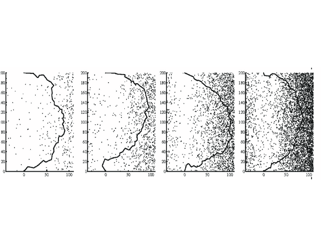
Figure 1: Minimum cost routes in increasingly large networks.

The term “massively dense” ad hoc networks is used to indicate not only that the number of nodes is large, but also that the network is highly connected. By the term “dense” we further understand that for every point in the plane there is a node close to it with high probability; by “close” we mean that its distance is much smaller than the transmission range. In this paper and in previous works (cited in the next paragraphs) one actually studies the limiting properties of massively dense ad hoc networks, as the density of nodes tends to infinity.

The empirical discovery of the macroscopic limits motivated a large number of researchers to investigate continuum-type limits of the routing problem. A very basic problem in doing so has been to identify the most appropriate scientific context for modelling and solving this continuum limit routing problem. Our major contribution is to identify completely the main paradigms (from optimal control as well as from road traffic engineering) for the modelling and the solution of this problem. We illustrate the use of these methodologies by considering new types of models that arise in the case of nodes with directional antennas.

Physics-inspired paradigms: The physics-inspired paradigms used for the study of large ad hoc networks go way beyond those related to statistical-mechanics in which macroscopic properties are derived from microscopic structure. Starting from the pioneering work by Jacquet (see [18]) in that area, a number of research groups have worked on massively dense ad hoc networks using tools from geometrical optics [18]. Popa et al. in [22] studied optical paths and actually showed that the optimal solution to a minmax problem of load balancing can be achieved by using an appropriately chosen optical profile. The forwarding load appears to correspond to the scalar sum of traffic flows of different classes. This means that the optimal solution (with respect to this objective) can be achieved by single path routes, a result obtained also in [15]. Similar problems have been also studied in [8], as well as in works doing load balancing by analogies to Electrostatics (see e.g. [13, 19, 20, 27, 28], and the survey [29] and references therein). We shall describe these in the next sections.

The physical paradigms allow the authors to minimize various metrics related to the routing problem. In contrast, Hyytia and Virtamo proposed in [16] an approach based on load balancing arguing that if shortest path (or cost minimization) arguments were used, then some parts of the network would carry more traffic than others and may use more energy than others. This would result in a shorter lifetime of the network since some parts would be out of energy earlier than others.

Road-traffic paradigms: The development of the original theory of routing in massively dense networks among the community of ad hoc networks has emerged in a complete independent way of the existing theory of routing in massively dense networks which had been developed within the community of road traffic engineers. Indeed, this approach had already been introduced in 1952 by Wardrop [31] and by Beckmann [4] and is still an active research area among that community, see [6, 7, 14, 17, 33] and references therein.

Our contribution and the paper’s structure: We combine in this paper various approaches from the area of road traffic engineering as well as from optimal control theory in order to formulate models for routing in massively dense networks. We further propose a simple novel approach to that problem using a classical device of 2-D, singular optimal control [21], based on Green’s formula to obtain a simple characterization of least cost paths of individual packets. We end the paper by a numerical example for computing an equilibrium.

The paper starts with a background on the research on massively dense ad hoc networks. In doing so, it is not limited to a specific structure of the cost. However, when introducing our approach based on road traffic tools, we choose to restrict ourselves to static networks (say sensor networks) having a special cost structure characterized by communications through horizontally and vertically oriented directional antennas. The use of directional antennas, by pointing information in a specific direction, allows one to save energy which may result in a longer life time of the network. The nodes are assumed to be placed deterministically. For an application of our approach to omnidirectional antennas, see [1]. We solve various types of optimization problems: We consider (i) the global optimization problem in which the objective of routing decisions is to minimize a global cost, (ii) the individual optimization problem whose solution is the Wardrop equilibrium. It corresponds to the situation where the number of users is very large, and each user tries to minimize its own cost (in a non-cooperative way). This is a “population game” or a “non-atomic-game” framework. It is called “non-atomic” since a single player sends a negligible amount of traffic (with respect to the total amount of traffic) and as a consequence, its impact on the performance of other users is negligible.

The structure of this paper is as follows: We begin by presenting models for costs relevant to optimization models in routing or to node assignment. We then formulate the global optimization problem and the individual optimization one with a focus on the directional antennas scenario. We provide several approaches obtaining both a qualitative characterization as well as quantitative solutions to the problems.

2 An overview of dense ad hoc networks

We suppose that the network is modeled in the two dimensional plane $X_{1}\times X_{2}$. The continuous information density function $\rho(\mathbf{x})$, measured in $\textrm{bps}/\textrm{m}^{2}$, at locations $\mathbf{x}$ where $\rho(\mathbf{x})>0$ corresponds to a distributed data origin such that the rate with which information is created in an infinitesimal area of size $dA_{\varepsilon}$ centered at $\mathbf{x}$ is $\rho(\mathbf{x})\,dA_{\varepsilon}$. Similarly, at locations $\mathbf{x}$ where $\rho(\mathbf{x})<0$ there is a distributed data sink such that the rate with which information is absorbed by an infinitesimal area of size $dA_{\varepsilon}$, centered at point $\mathbf{x}$, is equal to $-\rho(\mathbf{x})\,dA_{\varepsilon}$.

The total rate at which the destination nodes receive the data must be the same as the total rate at which the data is created at the origin nodes, i.e.,

$$\int\limits_{X_{1}\times X_{2}}\rho(\mathbf{x})\,dS=0.$$

In optimizing a routing protocol in ad hoc networks, or in optimizing the placement of nodes, one of the starting points is the determination of the cost function that captures the cost of transporting a packet through the network. To determine it, we need a detailed specification of the network which includes the following:

• A model for the placement of nodes in the network.

• A forwarding rule that nodes will use to select the next hop of a packet.

• A model for the cost incurred in one hop, i.e., for transmitting a packet to an intermediate node.

Below we present several ways of choosing cost functions.

We define the flow of information $\mathbf{T}(\mathbf{x})$ (see Fig. 2) to be a vector whose components are the horizontal and vertical flows at point $\mathbf{x}$. Throughout we assume that each point carries a single flow (although the methodology can be extended to the multiflow case). The restriction to a single flow is justified when there is either a single destination, or when there is a set of destination points and the routing protocol has the freedom to decide to which of the set the packets will be routed. Under this type of conditions, one may assume a single flow at each point without loss of optimality (see e.g. [15]).

\psfrag{T}{$\mathbf{T}(\mathbf{x})$}\psfrag{T1}{$T_{1}(\mathbf{x})$}\psfrag{T2}{$T_{2}(\mathbf{x})$}\psfrag{X1}{$X_{1}$}\psfrag{X2}{$X_{2}$}\psfrag{e}{$d\ell$}\includegraphics[height=144.54pt,width=158.99377pt]{Nuevas-Figuras/arrow-flow.eps}

Figure 2: Flow of information $\mathbf{T}(\mathbf{x})$ through incremental line segment $d\ell$, decomposed in its horizontal component $T_{1}(\mathbf{x})$ (in the direction $X_{1}$) and its vertical component $T_{2}(\mathbf{x})$ (in the direction $X_{2}$).

2.1 Costs derived from capacity scaling

Many models have been proposed in the literature that show how the transport capacity scales with the number of nodes $n$ or with the density of nodes $\lambda$ within a certain region. A typical cost (see e.g. [27]) considered at a neighborhood of a location $\mathbf{x}$ is the density of nodes required there to carry a given flow of information $\mathbf{T}(\mathbf{x})$. We will work within a general framework and then investigate deeply some particular cases with different possible protocols. Assume that we use a protocol that provides a transport capacity of the order of $f(\lambda)$ at some region in which the density of nodes is $\lambda$ (we will provide examples of the function $f$ ahead). This means that in order to support a flow of information $\lvert\mathbf{T}(\mathbf{x})\rvert$ passing through a neighborhood of the location $\mathbf{x}$, we will need to place deterministically the nodes according to the formula $f^{-1}(\lvert\mathbf{T}(\mathbf{x})\rvert)$. Then if we assume that a flow of information $\mathbf{T}(\mathbf{x})$ is assigned through a neighborhood of the location the cost will be taken as

$$c(\mathbf{x},\mathbf{T}(\mathbf{x}))=f^{-1}(\lvert\mathbf{T}(\mathbf{x})\rvert)$$ (1)

where $\lvert\cdot\rvert$ represents the norm of a vector.

Most work in this area has considered the $\ell^{2}$-norm, i.e., for $\mathbf{x}=(x_{1},x_{2})$, we define $\lvert\mathbf{x}\rvert=\sqrt{x_{1}^{2}+x_{2}^{2}}$. We shall consider later also the $\ell^{1}$-norm, i.e., $\lvert\mathbf{x}\rvert=\lvert x_{1}\rvert+\lvert x_{2}\rvert$.

Examples for $f$:

• Using a network theoretic approach based on multi-hop communication, Gupta and Kumar proved in [12] that the throughput of the system that can be transported by the network when the nodes are optimally located is $\Omega(\sqrt{\lambda})$, and when the nodes are randomly located this throughput becomes $\Omega(\frac{\sqrt{\lambda}}{\sqrt{\log\lambda}})$. Using percolation theory, the authors of [10] have shown that in the randomly located set the same $\Omega(\sqrt{\lambda})$ can be achieved.

• Baccelli, Blaszczyszyn and Mühlethaler introduce in [2] an access scheme, MSR (Multi-hop Spatial Reuse Aloha), reaching the Gupta and Kumar bound $\Theta(\sqrt{\lambda})$ which does not require prior knowledge of the node density.

We conclude that for the model of Gupta and Kumar with either the optimal location or the random location approaches, as well as for the MSR protocol with a Poisson distribution of nodes, we obtain a quadratic cost of the form

$$c(\mathbf{T}(\mathbf{x}))=k\lvert\mathbf{T}(\mathbf{x})\rvert^{2}=k(T_{1}({\bf x})^{2}+T_{2}({\bf x})^{2}).$$ (2)

This follows from the fact that in the previous examples $f(x)$ behaves like $\sqrt{x}$, so the inverse of the function $f$ must be quadratic. Then from (1) we conclude that the cost function must be quadratic on $\lvert\mathbf{T}(x)\rvert$.

2.2 Congestion independent routing

A metric often used in the Internet for determining routing costs is the number of hops from origins to destinations, which routing protocols try to minimize. The number of hops is proportional to the expected delay along the path in the context of ad hoc networks, in case the queueing delay is negligible with respect to the transmission delay over each hop. This criterion is insensitive to interference or congestion. We assume that it depends only on the transmission range. We describe various cost criteria that can be formulated with this approach.

• If the range is constant then the cost density $c(\mathbf{x})$ is constant so that the cost of a path is its length in meters. The routing then follows a shortest path selection.

• Let us assume that the range $R(\lambda;\mathbf{x})$ is small, and it depends on local radio conditions at position $\mathbf{x}$ (for example, if it is influenced by weather conditions) but not on interference. The latter is justified when dedicated orthogonal channels (e.g. in time or frequency) can be allocated to traffic flows that would otherwise interfere with each other. Then determining the optimal routing becomes a path cost minimization problem. We further assume, as in [12], that the range is scaled to go to $0$ as the total density $\lambda$ of nodes grows to infinity. More precisely, let us consider a scaling of the range such that the following limit exists:

  $$r(\mathbf{x}):=\lim_{\lambda\to\infty}\frac{R(\lambda;\mathbf{x})}{\lambda}$$

  Then in the dense limit, the fraction of nodes that participate in forwarding packets along a path is $1/r(\mathbf{x})$ at position $\mathbf{x}$, and the path cost is the integral of this density along the path.

• The influence of varying radio conditions on the range can be eliminated using power control that can equalize the hop distance.

2.3 Costs related to energy consumption

In the absence of capacity constraints, the cost can represent energy consumption. In a general multi-hop ad hoc network, the hop distance can be optimized so as to minimize the energy consumption. Even within a single cell of 802.11 IEEE wireless LAN one can improve the energy consumption by using multiple hops, as it has been shown not to be efficient in terms of energy consumption to use a single hop [23].

Alternatively, the cost can take into account the scaling of the nodes (as we have done in Section 2.1) that is obtained when there are energy constraints. As an example, assuming random deployment of nodes, where each node has data to send to another randomly selected node, the capacity (in bits per Joule) has the form $f(\lambda)=\Omega\left((\lambda/\log\lambda)^{(q-1)/2}\right)$ where $q$ is the path-loss, see [24]. The cost is then obtained using (1).

3 Preliminaries

In the work of Toumpis et al. ([13, 26, 27, 28, 29, 30]), the authors addressed the problem of the optimal deployment of wireless sensor networks by a parallel with Electrostatics. We shall recall below the representation of the flow conservation constraint, which is well known in Electrostatics. This derivation appears both in physics-inspired papers ([13, 26, 27, 28, 29, 30]) as well as in the road traffic literature [6].

Consider a grid area network $D_{0}$ of arbitrary shape on the two-dimensional plane with axis $X_{1}$ and axis $X_{2}$, with smooth boundary. It is necessary that the rate with which information is created in the area must be equal to the rate with which information is leaving that area, i.e.,

$$\int\limits_{D_{0}}\rho(\mathbf{x})\,d\mathbf{x}=\oint\limits_{\partial D_{0}}[\mathbf{T}(\mathbf{x})\cdot\mathbf{n}(\mathbf{x})]\,d\ell.$$ (3)

The integral on the left is the surface integral of $\rho(\mathbf{x})$ over $D_{0}$. The integral on the right is the path integral of the inner product $\mathbf{T}\cdot\mathbf{n}$ over the curve $\partial D_{0}$. The vector $\mathbf{n}(\mathbf{x})$ is the unit normal vector to $\partial D_{0}$ at the boundary point $\mathbf{x}\in\partial D_{0}$ and pointing outwards. The function $\mathbf{T}(\mathbf{x})\cdot\mathbf{n}(\mathbf{x})$, measured in $\textrm{bps}/\textrm{m}$, is equal to the rate with which information is leaving the domain $D_{0}$ per unit length of boundary at the boundary point $\mathbf{x}$.

As this holds for any (smooth) domain $D_{0}$, it follows that necessarily

$$\nabla\cdot\mathbf{T}(\mathbf{x}):=\frac{\partial{T}_{1}(\mathbf{x})}{\partial x_{1}}+\frac{\partial{T}_{2}(\mathbf{x})}{\partial x_{2}}=\rho(\mathbf{x}),$$ (4)

where “$\nabla\cdot$” is the divergence operator. Notice that equations (3) and (4) are the integral and differential versions of Gauss’s law, respectively.

Extension to multi-class traffic The work on massively dense ad hoc networks considers a single class of traffic. In the geometrical optics approach it corresponds to demand from a location $\mathbf{a}$ to a location $\mathbf{b}$. In the Electrostatic case it corresponds to a set of origins and a set of destinations where traffic from any origin point could go to any destination point. The analogy to positive and negative charges in Electrostatics may limit the perspectives of multi-class problems where traffic from distinct origin sets has to be routed to distinct destination sets.

The model based on geometrical optics can directly be extended to include multiple classes as there are no elements in the model that suggest coupling between classes. This is due in particular to the fact that the cost density has been assumed to depend only on the density of the nodes and not on the density of the flows.

In contrast, the cost in the model based on Electrostatics is assumed to depend both on the location as well as on the local flow density. It thus models more complex interactions that would occur if we considered the case of $\nu$ traffic classes. Extending the relation (4) to the multi-class case, we have traffic conservation at each point in space for each traffic class as expressed in the following:

$$\mathbf{\nabla}\cdot\mathbf{T}^{j}(\mathbf{x})=\rho^{j}(\mathbf{x}),\qquad\forall\mathbf{x}\in D.$$ (5)

The function $\mathbf{T}^{j}$ is the flow distribution of class $j$ and $\rho^{j}$ corresponds to the distribution of the external origin and/or destinations.

Let $\mathbf{T}(\mathbf{x})$ be the total flow vector at point $\mathbf{x}\in D$. It is a vector of dimension $\nu$, and each one of the $\nu$-entries is a two dimensionnal flow. A generic multi-class optimization problem would then be: minimize $Z$ over the flow distributions $\{\mathbf{T}^{j}\}$

$$Z=\int_{D}c(\mathbf{x},\mathbf{T}(\mathbf{x}))\,d\mathbf{x}\quad\mbox{subject to}\quad\mathbf{\nabla}\cdot\mathbf{T}^{j}(\mathbf{x})=\rho^{j}(\mathbf{x}),\ j=1,...,\nu\qquad\forall\mathbf{x}\in D.$$ (6)

4 Directional Antennas and Global Optimization

So far we have adopted a general framework under which the flow is conserved. To proceed, we need more specific assumptions on the cost function. The one we shall introduce here can be called an $\ell^{1}$-norm model, in which the cost to go from a point to another is the sum of the horizontal and vertical cost components. This is justified in case traffic flows only horizontally or vertically (so that even a continuous diagonal curve is understood as a limit of many horizontal and vertical displacements). In road traffic, this corresponds to a Manhattan-like network, see [6]. In the context of sensor networks this would correspond to directional antennas (either horizontal or vertical). An alternative approach based on road traffic tools that is adapted to omni-directional antennas can be found in [1, 25] and we call it the $L2$-norm (meaning that the cost at any point depends on the absolute value of the traffic there and not on its direction). An extensive discussions on methods for numerical solutions of our problem as well as the problem in [1] can be found in [25] and in references there in, as well as in [6].

4.1 The model

Nodes are placed (deterministically) in a large number. For energy efficiency, it is assumed that each node is equipped with one or with two directional antennas, allowing transmission at each hop to be directed either from North to South or from West to East. The model we use extends that of [6] to the multi-class framework. We thus consider $\nu$ classes of flows $T_{1}^{j}\geq 0,\ T_{2}^{j}\geq 0$, $j=1,...,\nu$. To be compatible with Dafermos [6], we use her definitions of orientation according to which the directions North to South and West to East are taken positive. In the dense limit, a curved path can be viewed as a limit of a path with many such hops as the hop distance tends to zero.

Some assumptions on the cost:

• Individual cost: We allow the cost for a horizontal transmission (West-to-East, or equivalently, in the direction of the axis $x_{1}$) to be different than the cost for a vertical transmission (North-to-South, or equivalently, in the direction of the axis $x_{2}$). It is assumed that a packet traveling in the direction of the axis $x_{1}$ incurs a transportation cost $g_{1}$, and equivalently, traveling in the direction of the axis $x_{2}$ incurs a transportation cost $g_{2}$. Notice that the transportation costs $g_{1}$ and $g_{2}$ depend on the location $\mathbf{x}$ and the traffic flow $\mathbf{T}(\mathbf{x})$ that is flowing through that location, i.e., $g_{1}=g_{1}(\mathbf{x},\mathbf{T}(\mathbf{x}))$ and $g_{2}=g_{2}(\mathbf{x},\mathbf{T}(\mathbf{x}))$.

• We consider a vector transportation cost $\mathbf{g}:=(g_{1},g_{2})$. Notice that as each of its components, such vector transportation cost depends also upon the location $\mathbf{x}$ and the traffic flow $\mathbf{T}(\mathbf{x})$ flowing through that location, i.e., $\mathbf{g}=\mathbf{g}(\mathbf{x},\mathbf{T}(\mathbf{x}))$.

• The local transportation cost $g$ for the global optimization problem is given by the inner product between the vector transportation cost and the flow of information, i.e.,

  $$g(\mathbf{x},\mathbf{T}(\mathbf{x}))=\mathbf{g}(\mathbf{x},\mathbf{T}(\mathbf{x}))\cdot\mathbf{T}(\mathbf{x})=g_{1}T_{1}+g_{2}T_{2},$$

  and it corresponds to the sum of the transportation costs multiplied by the quantity of flow in each direction.

• The global transportation cost is the integral of the local transportation cost over the domain, i.e., $\int_{D}g(\mathbf{x},\mathbf{T}(\mathbf{x}))\,d\mathbf{x}$.

• The local cost $g(\mathbf{x},\mathbf{T}(\mathbf{x}))$ is assumed to be non-negative, monotone increasing in each component of $\mathbf{T}$ ($T_{1}$ and $T_{2}$ in our $2$-dimensional case).

The boundary conditions will be determined by the options that travelers have in selecting their origin and/or destinations. Examples of the boundary conditions are:

• Assignment problem: users of the network have predetermined origin and destinations and are free to choose their travel paths.

• Combined distribution and assignment problem: users of the network have predetermined origins and are free to choose their destinations (within a certain destination region) as well as their paths.

• Combined generation, distributions and assignment problem: users are free to choose their origins, their destinations, as well as their travel paths.

The problem formulation is again to minimize $Z$ as defined in (6). The natural choice of functional spaces to make that problem precise, and to take advantage of the available theory developped in the PDE (Partial Differential Equations) community, is to work in the Sobolev space $H^{1}$. We define $L^{2}(D)$ as the space of functions that are square-integrable, i.e., $L^{2}(D)=\{f\text{ such that }\int_{D}\lvert f(\mathbf{x})\rvert^{2}\,d\mathbf{x}<+\infty\}$. We define $H^{1}(D)$ as the space of functions that are square integrable, and with weak gradient square-integrable. Take $f$ to be a scalar function, define its weak gradient as a vector function $g$ such that, for any smooth vector function $\phi$ with compact support in $D$, $\int_{D}f\ \nabla\cdot\phi=-\int_{D}<g,\phi>$. Then, we seek $T^{j}_{i}$ in $H^{1}(D)$, such that $\rho$ is in $L^{2}(D)$.

4.2 Karush-Kuhn-Tucker conditions

The Karush-Kuhn-Tucker conditions (also known as KKT conditions) which we introduce below are necessary conditions for a solution in nonlinear programming to be optimal. It is a generalization of the method of Lagrange multipliers. We recall that the method of Lagrange multipliers provides a strategy for finding the minimum of a function subject to constraints and it is based on introducing new variables called Lagrange multipliers and study a function called Lagrange function. If a traffic flow $\mathbf{T}$ is optimal for our global optimization problem then there exist Lagrange multipliers that satisfy some complementarity conditions such that the corresponding Lagrangian is maximized by $\mathbf{T}$.

In the problem considered here the traffic flow in each direction $T_{i}$ is a functional (a map from the vector space to the scalar space). Then we will consider variational inequalities, i.e., inequalities involving a functional which have to be solved for all the values of the vector space.

A key application of these KKT conditions will be introduced in Section 6. We study there the individual (non-cooperative) optimization problem for each packet sent through the network and show that the solution must satisfy some variational inequalities. We then show that these inequalities can be interpreted as the Karush-Kuhn-Tucker conditions that we introduce in this chapter, applied to some transformed cost (called “potential” and introduced by Beckmann [5]). This will allow us to propose a method for solving the individual (non-cooperative) optimization problem.

We begin by recalling Green’s Theorem which has proved to be useful for many physical phenomena. We will make extensive use of this theorem in this section as well as in Section 6.

Theorem 4.1 (Green’s Theorem)

Let $D$ be a region of the space, and let $\partial D$ be its piecewise-smooth boundary. Consider the scalar function $u$ and a continuously differentiable vector function $\mathbf{v}$, then

$$\int_{D}u\nabla\cdot\mathbf{v}dx=\int_{\partial D}u<\mathbf{v},\mathbf{n}>d\ell-\int_{D}<\mathbf{v},\nabla u>dx.$$

By making use of this theorem and the Karush-Kuhn-Tucker conditions we are able to prove a result that provides a characterization of the optimal solution for some special cases as we will see in the following.

Theorem 4.2

Define the Lagrangian as

$$L^{\zeta}(\mathbf{T}):=\int_{D}\ell^{\zeta}(\mathbf{x},\mathbf{T})\,d\mathbf{x}\quad\text{with}\quad\ell^{\zeta}(\mathbf{x},\mathbf{T}):=g(\mathbf{x},\mathbf{T})-\sum_{j=1}^{\nu}\zeta^{j}(\mathbf{x})\Big{[}\mathbf{\nabla}\!\cdot\!\mathbf{T}^{j}(\mathbf{x})-\rho^{j}(\mathbf{x})\Big{]}$$

where $\zeta^{j}(\mathbf{x})\in L^{2}(D)$ are called Lagrange multipliers.

For a vector field $\mathbf{T}(\cdot)$ with positive components satisfying (5), a necessary and sufficient condition for minimizing the cost (6) is that the Lagrangian be minimized over all vector fields with positive components, or equivalently, that equations

$$\frac{\partial g(\mathbf{x},\mathbf{T})}{\partial T_{i}^{j}}+\frac{\partial\zeta^{j}(\mathbf{x})}{\partial x_{i}} =0\quad\mbox{ if }\quad T_{i}^{j}(\mathbf{x})>0,$$ (7a)

$$\frac{\partial g(\mathbf{x},\mathbf{T})}{\partial T_{i}^{j}}+\frac{\partial\zeta^{j}(\mathbf{x})}{\partial x_{i}} \geq 0\quad\mbox{ if }\quad T_{i}^{j}(\mathbf{x})=0.$$ (7b)

be satisfied.

Proof.- The criterion is convex, and the constraint (5) affine. Therefore the Karush-Kuhn-Tucker theorem holds, stating that the Lagrangian is minimum at the optimum. A variation $\delta\mathbf{T}(\cdot)$ will be admissible if $\mathbf{T}(\mathbf{x})+\delta\mathbf{T}(\mathbf{x})\geq 0$ for all $\mathbf{x}$, hence in particular, for all $\mathbf{x}$ such that $T_{i}^{j}(\mathbf{x})=0$ and $\delta T_{i}^{j}(\mathbf{x})\geq 0$.

As we are working with functionals, we need a generalisation of the concept of directional derivative used in differential calculus. The Gâteaux differential $DF(u,d)$ of functional $F$ at $u$ in the direction $d$ is defined as

$$DF(u,d)=\lim_{t\to 0}\frac{F(u+td)-F(u)}{t}=\frac{d}{dt}F(u+td)\Big{|}_{t=0}.$$

if the limit exists. If the limit exists for all $d$, one says that $F$ is Gâteaux differentiable at $u$.

Let $\mathrm{D}L^{\zeta}$ denote the Gâteaux derivative of functional $L^{\zeta}$ with respect to $\mathbf{T}(\cdot)$. First order condition for local minimum reads

$$\text{For all }\delta\mathbf{T}\>\mbox{admissible}\>,\mathrm{D}L^{\zeta}\cdot\delta\mathbf{T}\geq 0\,,$$

therefore here

$$\int_{D}\sum_{j}\langle\nabla_{\mathbf{T}^{j}}g(\mathbf{x},\mathbf{T}(\mathbf{x})),\delta\mathbf{T}^{j}(\mathbf{x})\rangle\,d\mathbf{x}-\int_{D}\sum_{j}\zeta^{j}(\mathbf{x})\nabla\!\cdot\!\delta\mathbf{T}^{j}(\mathbf{x})\,d\mathbf{x}\geq 0.$$

Integrating by parts using Green’s Theorem, this is equivalent to

$$\int_{D}\sum_{j}\left[\langle\nabla_{\mathbf{T}^{j}}g,\delta\mathbf{T}^{j}\rangle+\langle\nabla_{\mathbf{x}}\zeta^{j},\delta\mathbf{T}^{j}\rangle\right]d\mathbf{x}-\int_{\partial D}\sum_{j}\zeta^{j}\langle\delta\mathbf{T}^{j},\mathbf{n}\rangle\,d\ell\geq 0\,.$$

We may choose all the components $\delta\mathbf{T}^{k}=0$ except $\delta\mathbf{T}^{j}$, and choose $\delta\mathbf{T}^{j}$ in $(H^{1}_{0}(D))^{2}$, i.e., functions in $H^{1}(D)$ such that their boundary integral be zero. This is always feasible and admissible. Then the last term above vanishes, and it is a classical fact that the inequality implies (7a)-(7b) for $i=1,2$.

Placing this back in Euler’s inequality, and using a $\delta\mathbf{T}^{j}$ non zero on the boundary, it follows that necessarily $\zeta^{j}(\mathbf{x})=0$ at any $\mathbf{x}$ of the boundary $\partial D$ where $T(\mathbf{x})>0$. As we shall see this conditions provides the boundary condition to recover the Lagrange multipliers $\zeta^{j}$ from equation (5).

Equation (7a)-(7b) is already stated in [6] for the single class case. However, as Dafermos states explicitly, its rigorous derivation is not available there. $\blacksquare$

Consider the following special cases that we shall need later. We assume a single traffic class, but this could easily be extended to several. Let

$$g(\mathbf{x},\mathbf{T}(\mathbf{x}))=\sum_{i=1,2}g_{i}(\mathbf{x},\mathbf{T}(\mathbf{x}))T_{i}(\mathbf{x}).$$

1. Monomial cost per packet:

   $$g_{i}(\mathbf{x},\mathbf{T}(\mathbf{x}))=k_{i}(\mathbf{x})\Big{(}T_{i}(\mathbf{x})\Big{)}^{\beta}$$ (8)

   for some $\beta>1$. Then (7a)-(7b) simplify to

   $$(\beta+1)k_{i}(\mathbf{x})\left(T_{i}(\mathbf{x})\right)^{\beta}+\frac{\partial\zeta(\mathbf{x})}{\partial x_{i}} =0\quad\mbox{ if }T_{i}(\mathbf{x})>0,$$ (9a)

   $$(\beta+1)k_{i}(\mathbf{x})\left(T_{i}(\mathbf{x})\right)^{\beta}+\frac{\partial\zeta(\mathbf{x})}{\partial x_{i}} \geq 0\quad\mbox{ if }T_{i}(\mathbf{x})=0.$$ (9b)

   In that case, recovery of $\zeta$ to complete the process is difficult, at best. Things are simpler in the next case.

2. Affine cost per packet:

   $$g_{i}(\mathbf{x},\mathbf{T}(\mathbf{x}))=\frac{1}{2}k_{i}(\mathbf{x})T_{i}(\mathbf{x})+h_{i}(\mathbf{x}).$$ (10)

   Then (7a)-(7b) simplify to

   $$k_{i}(\mathbf{x})T_{i}(\mathbf{x})+h_{i}(\mathbf{x})+\frac{\partial\zeta(\mathbf{x})}{\partial x_{i}} =0\quad\mbox{ if }T_{i}(\mathbf{x})>0,$$

   $$k_{i}(\mathbf{x})T_{i}(\mathbf{x})+h_{i}(\mathbf{x})+\frac{\partial\zeta(\mathbf{x})}{\partial x_{i}} \geq 0\quad\mbox{ if }T_{i}(\mathbf{x})=0.$$

   Assume that the $k_{i}(\cdot)$ are everywhere positive and bounded away from 0. For simplicity, let $a_{i}=1/k_{i}$, and $b$ be the vector with coordinates $b_{i}=h_{i}/k_{i}$, all assumed to be square integrable. Assume that there exists a solution where $T(\mathbf{x})>0$ for all $\mathbf{x}$. Then

   $$T_{i}(\mathbf{x})=-\left(a_{i}(\mathbf{x})\frac{\partial\zeta(\mathbf{x})}{\partial x_{i}}+b_{i}(\mathbf{x})\right).$$

   As a consequence, from (5) and the above remark, we get that $\zeta(\cdot)$ is to be found as the solution in $H^{1}_{0}(D)$ of the elliptic equation (an equality in $H^{-1}(D)$)

   $$\sum_{i}\frac{\partial}{\partial x_{i}}\left(a_{i}(\mathbf{x})\frac{\partial\zeta(\mathbf{x})}{\partial x_{i}}\right)+\nabla\!\cdot\!b(\mathbf{x})+\rho(\mathbf{x})=0\,.$$

   This is a well behaved Dirichlet problem, known to have a unique solution in $H^{1}_{0}(D)$, furthermore easy to compute numerically.

5 User optimization and congestion independent costs

In this section, we extend the shortest path approach for optimization that has already appeared using geometrical optics tools [18]. We present a general optimization framework for handling shortest path problems and more generally, minimum cost paths.

We consider the model of Section 4. We assume that the local cost depends on the direction of the flow but not on its size. The cost is $c_{1}(\mathbf{x})$ for a flow that is locally horizontal and is $c_{2}(\mathbf{x})$ for a flow that is locally vertical. We assume in this section that $c_{1}$ and $c_{2}$ do not depend on $\mathbf{T}$. The cost incurred by a packet transmitted along a path $p$ is given by the line integral

$$\mathbf{c}_{p}=\int_{p}\mathbf{c}\cdot\,d\mathbf{x}.$$ (12)

Let $V^{j}(\mathbf{x})$ be the minimum cost to go from a point $\mathbf{x}$ to a set $B^{j}$, $j=1,...,\nu$. Then

$$V^{j}(\mathbf{x})=\min\left(c_{1}(\mathbf{x})\,dx_{1}+V^{j}(x_{1}+\,dx_{1},x_{2}),c_{2}(\mathbf{x})\,dx_{2}+V^{j}(x_{1},x_{2}+\,dx_{2})\right).$$ (13)

This can be written as the Hamilton Jacobi Bellman (HJB) equation:

$$0=\min\left(c_{1}(\mathbf{x})+\frac{\partial V^{j}(\mathbf{x})}{\partial x_{1}},c_{2}(\mathbf{x})+\frac{\partial V^{j}(\mathbf{x})}{\partial x_{2}}\right),\qquad\forall\mathbf{x}\in B^{j}\,,\>V^{j}(\mathbf{x})=0\,.$$ (14)

If $V^{j}$ is differentiable then, under suitable conditions, it is the unique solution of (14). In the case that $V^{j}$ is not everywhere differentiable then, under suitable conditions, it is the unique viscosity solution of (14) (see [3, 9]).

There are many numerical approaches for solving the Hamilton-Jacobi-Bellman (HJB) equation. One can discretize the HJB equation and obtain a discrete dynamic programming for which efficient solution methods exist. If one repeats this for various discretization steps, then we know that the solution of the discrete problem converges to the viscosity solution of the original problem (under suitable conditions) as the step size converges to zero [3].

5.1 Geometry of minimum cost paths

We consider now our directional antenna model in a given rectangular area $R$, defined by the simple closed curve $\Gamma_{1}\cup\Gamma_{2}\cup\Gamma_{3}\cup\Gamma_{4}$ (see Fig. 4). We study the case where transmissions can go from North to South or from West to East.

We obtain below optimal paths defined as paths that achieve the minimum packet transmission cost defined by (12). We shall study two problems:

• Point to point optimal path: we seek the minimum cost path between two points.

• Point to boundary optimal path: we seek the minimum cost path on a given region that starts at a given point and is allowed to end at any point on the boundaries.

Another formulation of Green’s Theorem stated previously as Theorem 4.1 give us a characterization of the optimal paths for those two problems.

Theorem 5.1 (Green’s Theorem: alternative version)

Let $D$ be a region of the space, and let $\partial D$ be its piecewise-smooth boundary. Suppose that $P$ and $Q$ are continuously differentiable functions in $D$. Then

$$\oint_{\partial D}Pdx+Qdy=\int_{D}\left(\frac{\partial Q}{\partial x}-\frac{\partial P}{\partial y}\right)dxdy.$$

Recall that the cost is composed of a horizontal and a vertical component (these are $c_{1}({\bf x})$ and $c_{2}({\bf x})$ respectively), which are constant (do not depend on the flow size).

Consider the function

$$U(\mathbf{x})=\frac{\partial c_{2}}{\partial x_{1}}(\mathbf{x})-\frac{\partial c_{1}}{\partial x_{2}}(\mathbf{x}).$$

It will turn out that the structure of the minimum cost path depends on the costs through the sign of the function $U$. Now, if the function $\mathbf{c}$ is continuously differentiable then $U$ is a continuous function. This motivates us to study cases in which $U$ has the same sign everywhere (see Fig. 4), or in which there are two regions in the rectangle $R$, one with $U>0$ and one with $U<0$, separated by a curve $\ell$ on which $U=0$ (e.g. Fig. 4).

Figure 3: The rectangle $R$ defined by the boundaries $\Gamma_{1}\cup\Gamma_{2}\cup\Gamma_{3}\cup\Gamma_{4}$. The case where $U>0$.

Figure 4: The case of two regions separated by a curve. Case 1.

We shall assume throughout that the function $\mathbf{c}$ is continuously differentiable, and that, if non-empty, the set of points inside the domain where the function $U$ is zero, i.e., $\ell=\{\mathbf{x}\,:\,U(\mathbf{x})=0\}$, is a smooth line. (This is true, e.g., if $\mathbf{c}$ is a smooth function and $\nabla U\neq 0$ on $\ell$.)

5.2 The function $U$ has the same sign over the whole region

Theorem 5.2

(Point to point optimal path) Suppose that an origin point $\mathbf{x}^{o}=(x_{1}^{o},x_{2}^{o})$ wants to send a packet to a destination point $\mathbf{x}^{d}=(x_{1}^{d},x_{2}^{d})$ and both points are in the interior of rectangle $R$.

1. If the function $U$ is positive almost everywhere in the interior rectangle $R_{od}$ defined by both points (see Fig. 5(a)), then the optimal path $\gamma_{\rm opt}$ is given by a horizontal straight line $\gamma_{H}$ and then a vertical straight line $\gamma_{V}$ (see Fig. 5(a)).

   More precisely, $\gamma_{\rm opt}=\gamma_{H}\cup\gamma_{V}$ where

   $$\gamma_{H}=\{(x_{1},x_{2})\text{ such that }x_{1}^{o}\leq x_{1}\leq x_{1}^{d},x_{2}=x_{2}^{o}\},$$

   $$\gamma_{V}=\{(x_{1},x_{2})\text{ such that }x_{1}=x_{1}^{d},x_{2}^{o}\leq x_{2}\leq x_{2}^{d}\}.$$

2. If the function $U$ is negative almost everywhere in the interior rectangle $R_{od}$ then there is an optimal path $\gamma_{\rm opt}$ given by a vertical straight line $\gamma_{V}$ and then a horizontal straight line $\gamma_{H}$ (see Fig. 5(b)).

   More precisely, $\gamma_{\rm opt}=\gamma_{V}\cup\gamma_{H}$ where

   $$\gamma_{V}=\{(x_{1},x_{2})\text{ such that }x_{1}=x_{1}^{o},x_{2}^{o}\leq x_{2}\leq x_{2}^{d}\},$$

   $$\gamma_{H}=\{(x_{1},x_{2})\text{ such that }x_{1}^{o}\leq x_{1}\leq x_{1}^{d},x_{2}=x_{2}^{d}\}.$$

3. In both cases, $\gamma^{\text{opt}}$ is unique almost surely (i.e., the area between $\gamma^{\text{opt}}$ and any other optimal path is zero).

Proof.- Consider an arbitrary path $\gamma_{C}$ joining $\mathbf{x}^{o}$ to $\mathbf{x}^{d}$, and assume that the Lebesgue measure of the area between $\gamma^{\text{opt}}$ and $\gamma_{C}$ is nonzero. We call $\gamma_{C}$ the comparison path (see Fig. 5(a) for the case $U>0$ and Fig. 5(b) for the case $U<0$).

(a) Case $U>0$.

(b) Case $U<0$.

Figure 5: Optimal paths when $U>0$ 5(a) and when $U<0$ 5(b) in the interior rectangle defined by the origin point and the destination point.

(i) Showing that the cost over path $\gamma_{\rm opt}$ is optimal is equivalent to showing that the integral of the cost over the closed path $\mathcal{P}$ is negative. Hereby $\mathcal{P}$ is given by following $\gamma^{\text{opt}}$ from the origin $\mathbf{x}^{o}$ to the destination $\mathbf{x}^{d}$, and then returning from the destination $\mathbf{x}^{d}$ to the origin $\mathbf{x}^{o}$ by moving along the comparison path $\gamma_{C}$ in the reverse direction. This closed path is written as $\mathcal{P}=\gamma_{\rm opt}\cup\gamma_{C}^{-}$ and $A$ denotes the bounded area described by $\mathcal{P}$. Using Green’s Theorem we obtain

$$\oint_{\mathcal{P}}\mathbf{c}\cdot\mathbf{dx}=-\int_{A}U(\mathbf{x})dS$$

which is strictly negative since $U>0$ almost everywhere on the interior rectangle $R_{od}$. Decomposing the left integral, this concludes the proof of (i), and establishes at the same time the corresponding statement on uniqueness in (iii).
(ii) is obtained similarly. $\blacksquare$

Theorem 5.3

(Point to boundary optimal path)
Consider the problem of finding an optimal path from a point $\mathbf{x}^{o}$ in the rectangle $R$ to the boundary $\Gamma_{1}\cup\Gamma_{2}$.

1. If the function $U$ is almost everywhere negative inside the rectangle $R$ and the cost on the boundary $\Gamma_{1}$ is non-negative and on boundary $\Gamma_{2}$ is non-positive, then the optimal path is the straight vertical line (See Fig. 7).

2. If the function $U(\mathbf{x})$ is almost everywhere positive inside the rectangle $R$ and the cost on the boundary $\Gamma_{1}$ is non-positive and on boundary $\Gamma_{2}$ is non-negative. Then the optimal path is the straight horizontal line (See Fig. 7).

Proof.-

(i) Denote by $\gamma_{\rm opt}$ the straight vertical path joining $\mathbf{x}^{o}$ to the boundary $\Gamma_{1}$. Consider another arbitrary valid path $\gamma_{C}$ joining $\mathbf{x}^{o}$ to any point ${\bf x}^{*}$ on the boundary $\Gamma_{1}\cup\Gamma_{2}$, and assume that the Lebesgue measure of the area between $\gamma_{\text{opt}}$ and $\gamma_{C}$ is nonzero. We call $\gamma_{C}$ the comparison path.

Assume first that ${\bf x}^{*}$ is on the boundary $\Gamma_{2}$. Denote ${\bf x}^{D}$ the South-East corner of the rectangle $R$, i.e., ${\bf x}^{D}:=\Gamma_{1}\cap\Gamma_{2}$. Then by Theorem 5.2(ii), the cost to go from $\mathbf{x}^{o}$ to $\mathbf{x}^{d}$ is smaller when using $\gamma_{\rm opt}$ and then continuing eastwards (along $\Gamma_{1}$) than when using the comparison path $\gamma_{C}$ and then southwards (along $\Gamma_{2}$). Due to our assumptions on the costs over the boundaries, this implies that the cost along the straight vertical path $\gamma_{\rm opt}$ is smaller than along the comparison path $\gamma_{C}$.

Next consider the case where $\mathbf{x}^{*}$ is on the boundary $\Gamma_{1}$. Denote by $\eta$ the section of the boundary $\Gamma_{1}$ that joins $\gamma_{\rm opt}\cap\Gamma_{1}$ with $\mathbf{x}^{*}$ (see Figure 7). Then again, by Theorem 5.2 (ii), the cost to go from $\mathbf{x}^{o}$ to $\mathbf{x}^{*}$ is smaller when using $\gamma_{\rm opt}$ and then continuing eastwards (along $\Gamma_{1}$) than when using the comparison path $\gamma_{C}$. Due to our assumptions that the cost on $\Gamma_{1}$ is non-negative, this implies that the cost along $\gamma_{V}$ is smaller than along $\gamma_{C}$.

Figure 6: Theorem 5.3 (i)

Figure 7: Theorem 5.3 (ii)

(ii) is obtained similarly. $\blacksquare$

5.3 The function $U$ changes sign within the region $R$

Consider the region on the space $\ell:=\left\{\mathbf{x}\in R\text{ such that }U(\mathbf{x})=0\right\}.$ Let us consider the case when $\ell$ is a valid path in the rectangular area, such that it starts at the North-West corner (the intersection of the boundaries $\Gamma_{3}\cap\Gamma_{4}$) and finishes at the South-East corner (the intersection of the boundaries $\Gamma_{1}\cap\Gamma_{2}$). Then the space is divided in two areas, and as the function $U$ is continuous we have the following cases:

1. $U(\mathbf{x})$ is negative in the upper area and positive in the lower area (see Fig. 4).

2. $U(\mathbf{x})$ is positive in the upper area and negative in the lower area.

The two other cases where the sign of $U$ is the same over $R$ are contained in what we solved in the previous subsection 5.2.

Case 1: The function $U(\mathbf{x})$ is negative in the upper area and positive in the lower area.

We shall show that in this case, $\ell$ is an attractor, in the sense that the optimal path reaches the line $\ell$ with the minimal possible distance and then continues along this line until it reaches the destination.

Proposition 5.1

Assume that the origin point $\mathbf{x}^{o}$ and the destination point $\mathbf{x}^{d}$ are both on $\ell$. Then the path $p_{\ell}$ that follows $\ell$ from the origin point $\mathbf{x}^{o}$ to the destination point $\mathbf{x}^{d}$ is optimal.

Proof.- Consider a comparison path $\gamma_{C}$ that coincides with $\ell$ only in the origin $\mathbf{x}^{o}$ and destination $\mathbf{x}^{d}$ points. First assume that the comparison path $\gamma_{C}$ is entirely in the upper (i.e., northern) part and call $A$ the area between $\gamma_{C}$ and $p_{\ell}$. Define $\mathcal{P}$ to be the closed path that follows $p_{\ell}$ from $\mathbf{x}^{o}$ to $\mathbf{x}^{d}$ and then returns along $\gamma_{C}$.

The integral $\int_{A}U(\mathbf{x})\,d\mathbf{x}$ is negative by assumption. By Green’s Theorem, it is equal to  $\oint_{\mathcal{P}}\mathbf{c}\cdot\,d\mathbf{x}$. This implies that the cost along $p_{\ell}$ is strictly smaller than along $\gamma_{C}$.

A similar argument holds for the case that $\gamma_{C}$ is below $p_{\ell}$.

A path between $\mathbf{x}^{o}$ and $\mathbf{x}^{d}$ may have several intersections with $\ell$. Between each pair of consecutive intersections of $\ell$, the subpath has a cost larger than that obtained by following $\ell$ between these points (this follows from the previous steps of the proof). We conclude that $p_{\ell}$ is indeed optimal. $\blacksquare$

Proposition 5.2

Let an origin point $\mathbf{x}^{o}$ send packets to a destination point ${\bf x}^{D}$.

1. Assume both points are in the upper region. Denote by $\gamma_{1}$ the two segments path given by Theorem 5.2 (ii). Then the optimal curve $\gamma_{\rm opt}$ is obtained as the maximum between $\ell$ and $\gamma_{1}$.

2. Let both points be in the lower region. Denote by $\gamma_{2}$ the two segments path given in Theorem 5.2 (i). Then the optimal curve $\gamma_{\rm opt}$ is obtained as the minimum between $\ell$ and $\gamma_{2}$.

Proof.-

(i) A straightforward adaptation of the proof of the previous proposition implies that the path in the statement of the proposition is optimal among all those restricted to the upper region. Consider now a path $\gamma_{C}$ that is not restricted to the upper region. Then $\ell\cap\gamma_{C}$ contains two distinct points such that $\gamma_{C}$ is strictly lower than $\ell$ between these points. Applying Proposition 5.1, we then see that the cost of $\gamma_{C}$ can be strictly improved by following $\ell$ between these points instead of following $\gamma_{C}$ there. This concludes (i).

(ii) Proved similarly. $\blacksquare$

Proposition 5.3

Let a point $\mathbf{x}^{o}$ send packets to a point $\mathbf{x}^{d}$.

1. Assume the origin is in the upper region and the destination in the lower one. Then the optimal path has three segments;

   1. It goes straight vertically from $\mathbf{x}^{o}$ to $\ell$,

   2. Continues as long as possible along $\ell$, i.e., until it reaches the first coordinate of the destination,

   3. At that point it goes straight vertically from $\ell$ to $\mathbf{x}^{d}$.

2. Assume the origin is in the lower region and the destination in the upper one. Then the optimal path has three segments;

   1. It goes straight horizontally from $\mathbf{x}^{o}$ to $\ell$,

   2. Continues as long as possible along $\ell$, i.e., until it reaches the second coordinate of the destination,

   3. At that point it goes straight horizontally from $\ell$ to $\mathbf{x}^{d}$.

Proof.- The proofs of (i) and of (ii) are the same. Consider an alternative route $\gamma_{C}$. Let $\tilde{\bf x}$ be some point in $\gamma_{C}\cap\ell$. The proof now follows by applying the previous proposition to obtain first the optimal path between the origin and $\tilde{\bf x}$ and second, the optimal path between $\tilde{\bf x}$ and the destination. $\blacksquare$

Case 2: The function $U$ is positive in the upper area and negative in the lower area.

This case turns out to be more complex than the previous one. The curve $M$ has some obvious repelling properties which we state next, but they are not as general as the attractor properties that we had in the previous case.

Proposition 5.4

Assume that both origin and destination are in the same region. Then the paths that were optimal in Theorem 5.2 are optimal here as well, if we restrict ourselves to paths that remain in the same region.

Proof.- Given that the origin and destination are in a region we may change the cost over the other region so that it has the same sign over all the region $R$. This does not influence the cost of path restricted to the region of the origin-destination pair. With this transformation we are in the scenario of Theorem 5.2 which we can then apply. $\blacksquare$

Discussion.- Note that the (sub)optimal policies obtained in Proposition 5.4 indeed look like being repelled from $\ell$; their two segments trajectory guarantees to go from the origin to the destination as far as possible from $\ell$.

We note that unlike the attracting structure that we obtained in Case 1, one cannot extend the repelling structure to the case where the paths are allowed to traverse from one region to another.

6 User optimization and congestion dependent cost

We now go beyond the approach of the previous section by allowing the cost to depend on congestion. Shortest path costs can be a system objective as we shall motivate below. But it can also be the result of decentralized decision making by many “infinitesimally small” players where a player may represent a single packet (or a single session) in a context where there is a huge population of packets (or of sessions). The result of such a decentralized decision making can be expected to satisfy the following properties which define the so called, user (or Wardrop) equilibrium:

“Under equilibrium conditions traffic arranges itself in congested networks such that all used routes between an OD pair (origin-destination pair) have equal and minimum costs while all unused routes have greater or equal costs” [31].

Motivation.- One popular objective in some routing protocols in ad hoc networks is to assign routes for packets in a way that each packet follows a minimal cost path (given the others’ paths choices) [11]. This has the advantage of equalizing origin-destination delays of packets that belong to the same class, which allows one to minimize the amount of packets that come out of sequence (this is desirable since in data transfers, out of order packets are misinterpreted to be lost which results not only in retransmissions but also in drop of systems throughput).

Related work.- Both the framework of global optimization as well as the one of minimum cost path have been studied extensively in the context of road traffic engineering. The use of a continuum network approach was already introduced on 1952 by Wardrop [31] and by Beckmann [4]. For more recent papers in this area, see e.g. [6, 7, 14, 17, 33] and references therein. We formulate it below and obtain some of its properties.

Congestion dependent cost.- We allow the individual transmission cost $c_{1}$ for a horizontal transmission (in the direction of the axis $x_{1}$) to be different than the individual transmission cost $c_{2}$ for a vertical transmission (in the direction of the axis $x_{2}$). We add to the individual transmission cost $c_{1}$ the dependence on the traffic flow $T_{1}$ (in the direction of the axis $x_{1}$) and to the individual transmission cost $c_{2}$ the dependence on the traffic flow $T_{2}$ (in the direction of the axis $x_{2}$), as we did in Section 4 to the transportation cost for the global optimization problem.

Let $V^{j}(\mathbf{x})$ be the minimum cost to go from a point $\mathbf{x}$ to $B^{j}$ at equilibrium. Equation (13) still holds but this time with $c_{i}$ that depends on $T_{1}^{j}$, $T_{2}^{j}$, and on the total flows $T_{1}$, $T_{2}$. Thus (14) becomes, for all $j\in\{1,\ldots,\nu\}$,

$$0=\min_{i=1,2}\Big{(}c_{i}(\mathbf{x},T_{i})+\frac{\partial V^{j}(\mathbf{x})}{\partial x_{i}}\Big{)}\,,\quad\forall\mathbf{x}\in B^{j}\,,V^{j}(\mathbf{x})=0\,.$$ (15)

Notice that this method can be viewed as a generalization of the optimization method known as dynamic programming, in particular, last equation would be a generalization of Bellman equation also known as dynamic programming equation.

We note that if $T_{i}^{j}(\mathbf{x})>0$ then by the definition of the equilibrium, $i$ attains the minimum at (15). Hence (15) implies the following relations for each traffic class $j$, and for $i=1,2$:

$$c_{i}(\mathbf{x},T_{i})+\frac{\partial V^{j}}{\partial x_{i}}=0\quad\textrm{if}\quad T_{i}^{j}>0,$$ (16a)

$$c_{i}(\mathbf{x},T_{i})+\frac{\partial V^{j}}{\partial x_{i}}\geq 0\quad\textrm{if}\quad T_{i}^{j}=0.$$ (16b)

This is a set of coupled PDE’s (Partial Differential Equations), actually difficult to analyse further.

Beckmann transformation
As Beckmann et al. did in [5] for discrete networks, we transform the minimum cost problem into an equivalent global minimization one. We shall restrict our analysis to the single class case. To that end, we note that equations (16a)-(16b) have exactly the same form as the Karush-Kuhn-Tucker conditions (7a)-(7b), except that $c_{i}(\mathbf{x},T_{i})$ in the former are replaced by ${\partial g(\mathbf{x},\mathbf{T})}/{\partial T_{i}(\mathbf{x})}$ in the latter. We therefore introduce a potential function $\psi$ defined by

$$\psi(\mathbf{x},\mathbf{T})=\sum_{i=1,2}\int_{0}^{T_{i}}\!c_{i}(\mathbf{x},s){\rm d}s$$

so that for both $i=1,2$:

$$c_{i}(\mathbf{x},T_{i})=\frac{\partial\psi(\mathbf{x},\mathbf{T})}{\partial T_{i}}\,.$$

Then the user equilibrium flow is the one obtained from the global optimization problem where we use $\psi(\mathbf{x},\mathbf{T})$ as local cost. We conclude the following.

Theorem 6.1

Let $x^{*}$ be a solution to the following global optimization problem.

$$\min_{T(\cdot)}\int_{D}\psi(\mathbf{x},\mathbf{T})\,d\mathbf{x}\qquad\mbox{subject to }\mathbf{\nabla}\cdot\mathbf{T}(\mathbf{x})=\rho(\mathbf{x}),\qquad\forall\mathbf{x}\in D.$$

Then it is the Wardrop equilibrium.

Remark 6.1

In the special case where costs are given as a power of the flow as defined in eq. (8), we observe that equations (16a)-(16b) coincide with equations (9a)-(9b) (up-to a multiplicative constant of the cost). We conclude that for such costs, the user equilibrium and the global optimization solution coincide.

7 Example

The following example is an adaptation of the road traffic problem solved by Dafermos in [6] to our ad hoc setting. We therefore use the notation of [6] for the orientation, as we did in Section 4. Thus the direction from North to South will be our positive $x_{1}$ axis, and from West to East will be the positive $x_{2}$ axis. The framework we study is the user optimization problem with congestion dependent cost. For each point on the West and/or North boundary we consider the point to boundary problem. We thus seek a Wardrop equilibrium where each user can choose its destination among a given set. A flow configuration is a Wardrop equilibrium if under this configuration, each origin chooses a destination and a path to that destination that minimize that user’s cost among all its possible choices.

Consider the rectangular area $R$ on the bounded domain $D$ defined by the simple closed curve $\partial R^{+}=\Gamma_{1}^{+}\cup\Gamma_{2}^{+}\cup\Gamma_{3}^{-}\cup\Gamma_{4}^{-}$ where

$$\begin{array}[]{ll}\Gamma_{1}=\left\{0\leq x_{1}\leq a,\quad x_{2}=0\right\},&\Gamma_{2}=\left\{x_{1}=a,\quad 0\leq x_{2}\leq b\right\},\\ \Gamma_{3}=\left\{0\leq x_{1}\leq a,\quad x_{2}=b\right\},&\Gamma_{4}=\left\{x_{1}=0,\quad 0\leq x_{2}\leq b\right\}.\end{array}$$

Assume throughout that $\rho=0$ for all ${\mathbf{x}}$ in the interior of $D$, and that the costs of the routes are linear, i.e.,

$$c_{1}=k_{1}T_{1}+h_{1}\quad\textrm{and}\quad c_{2}=k_{2}T_{2}+h_{2},$$ (17)

with $k_{1}>0$, $k_{2}>0$, $h_{1}$, and $h_{2}$ constant over $D$. Linear costs can be viewed as a Taylor approximation of an arbitrary cost in the light traffic regime.

We are precisely in the framework of Section 4 and Section 6 with affine costs per packet. As a matter of fact, the potential function associated with these costs is

$$\psi(\mathbf{T})=\sum_{i=_{1}}^{2}\int_{0}^{T_{i}}(k_{i}s+h_{i})\,ds=\sum_{i=1}^{2}(\frac{1}{2}k_{i}T_{i}+h_{i})T_{i}\,.$$

Now, we want to handle a condensation of origins or destinations along the boundary. While this is feasible with the framework of section 4, it is rather technical. We rather use a more direct path below.

Notice that in the interior of $D$, we have

$$\frac{\partial T_{1}}{\partial x_{1}}+\frac{\partial T_{2}}{\partial x_{2}}=0.$$

Take any closed path $\gamma$ surrounding a region $\omega$. Then by Green formula,

$$\oint_{\gamma}T_{1}d\mathcal{P}_{2}-T_{2}d\mathcal{P}_{1}=\int_{\omega}\frac{\partial T_{1}}{\partial x_{1}}+\frac{\partial T_{2}}{\partial x_{2}}=0$$

Therefore we can define

$$\phi({\bf x}):=\int_{{\bf x^{o}}}^{\bf x}T_{1}d\mathcal{P}_{2}-T_{2}d\mathcal{P}_{1}$$

the integral will not depend on the path between ${{\bf x^{o}}}$ and ${\bf x}$ and $\phi$ is thus well defined, and we have

$$\frac{\partial\phi({\bf x})}{\partial x_{2}}=T_{1}({\bf x})\qquad\frac{\partial\phi({\bf x})}{\partial x_{1}}=-T_{2}({\bf x})\,.$$ (18)

We now make the assumption that there is sufficient demand and that the congestion cost is not too high so that at equilibrium the traffic $T_{1}$ and $T_{2}$ are strictly positive over all $D$ [6]. It turns out that all paths to the destination are used. Thus, from Wardrop’s principle, the cost $\int\!\mathbf{c}\,dx$ is equalized between any two paths. And therefore,

$$\frac{\partial c_{1}}{\partial x_{2}}=\frac{\partial c_{2}}{\partial x_{1}}.$$

Using the equations in (17) then

$$k_{1}\frac{\partial T_{1}}{\partial x_{2}}=k_{2}\frac{\partial T_{2}}{\partial x_{1}},$$

and from equations in (18) we have

$$k_{1}\frac{\partial^{2}\phi}{\partial x_{2}^{2}}+k_{2}\frac{\partial^{2}\phi}{\partial x_{1}^{2}}=0.$$

Let $k_{i}=K_{i}^{2}$. Divide the above equation by $k_{1}k_{2}$. One obtains

$$\frac{1}{K_{1}^{2}}\frac{\partial^{2}\phi}{\partial x_{1}^{2}}+\frac{1}{K_{2}^{2}}\frac{\partial^{2}\phi}{\partial x_{2}^{2}}=0.$$

Following the classical way of analyzing the Laplace equation, (see[32]) we attempt a separation of variables according to

$$\phi(x_{1},x_{2})=F_{1}(K_{1}x_{1})F_{2}(K_{2}x_{2})\,.$$

We then get that

$$\frac{F_{1}^{\prime\prime}(K_{1}x_{1})}{F_{1}(K_{1}x_{1})}=-\frac{F_{2}^{\prime\prime}(K_{2}x_{2})}{F_{2}(K_{2}x_{2})}=s^{2}\,.$$

In that formula, since the first term is independent on $x_{2}$ and the second on $x_{1}$, then both must be constant. We call $s^{2}$ that constant, but we do not know its sign. Therefore, $s$ may be imaginary or real. All solutions of this system for a given $s$ are of the form

$$F_{1}(x)=A\cos(isx)+B\sin(isx)\,,\qquad F_{2}=C\cos(sx)+D\sin(sx)\,.$$

As a matter of fact, $\phi$ may be the sum of an arbitrary number of such multiplicative decompositions with different $s$. We therefore arrive at the general formula

$$\phi(x_{1},x_{2})=\!\int\![A(s)\cos(isK_{1}x_{1})+B(s)\sin(isK_{1}x_{1})][C(s)\cos(sK_{2}x_{2})+D(s)\sin(sK_{2}x_{2})]\,ds.$$

From this formula, we can write $T_{1}$ and $T_{2}$ as integrals also. The flow $T$ at the boundaries should be orthogonal to the boundary, and have the local origin density for inward modulus (it is outward at a sink). It remains to expand these boundary conditions in Fourier integrals to identify the functions $A$, $B$, $C$, and $D$, which is tedious but straightforward (it is advisable to represent the integrals of the boundary densities as Fourier integrals, since then the boundary conditions themselves will be of the form $s\!\int\!R(s)\,ds$, closely matching the formulas we obtain for the $T_{i}$’s).

8 Conclusions

Routing in ad hoc networks has received much attention in the massively dense limit. The main tools to describe the limits had been Electrostatics and geometric optics. We exploited another approach for the problem that has its roots in road traffic theory, and presented both quantitative as well as qualitative results for various optimization frameworks. The links to road traffic theory allow us to benefit of the results of more than fifty years of research in that area that not only provide mature theoretical tools but have also advanced in numerical solution methods.

The continuum topology that we used in this paper is to be viewed as an approximation for dense networks. However, we believe that it may arise in other applications as well. As an example, consider a standard routing problem, in which instead of having a fixed rate of packets arrivals, we only have a constraint on the total amount of arrivals of packets, and then one has to choose both the instantaneous routes as well as at what (time-dependent) rate to transmit the packets. This type of problem (also much studied in road traffic context) can be viewed as routing over a continuum topology where time replaces space.

References

- [1] E. Altman, P. Bernhard, and A. Silva, “The Mathematics of Routing in Massively Dense Ad Hoc Networks,” 7th International Conference on Ad Hoc Networks and Wireless, September 10 - 12, 2008, Sophia Antipolis, France.
- [2] F. Baccelli, B. Blaszczyszyn, and P. Muhlethaler, “An ALOHA protocool for multihop mobile wireless networks,” IEEE Transactions on Information Theory, Vol. 52, Issue. 2, 421- 436, February 2006.
- [3] M. Bardi and I. Capuzzo-Dolcetta, Optimal Control and Viscosity Solutions of Hamilton-Jacobi-Bellman Equations, Birkhauser, 1994.
- [4] M. Beckmann, “A continuum model of transportation,” Econometrica 20:643–660, 1952.
- [5] M. Beckmann, C.B. McGuire and C.B. Winsten, Studies in the Economics and Transportation, Yale Univ. Press, 1956.
- [6] S. C. Dafermos, “Continuum Modeling of Transportation Networks,” Transpn Res. Vol. 14B, pp. 295–301, 1980.
- [7] P. Daniele and A. Maugeri, “Variational Inequalities and discrete and continuum models of network equilibrium protocols,” Mathematical and Computer Modelling 35:689–708, 2002.
- [8] E. Durocher, E. Kranakis, D. Krizanc, and L. Narayanan, “Balancing Traffic Load Using One-Turn Rectilinear Routing”, TAMC 2008. Lecture Notes in Computer Science, Springer Berlin, Heidelberg, Vol. 4978/2008, Theory and Applications of Models of Computation, pp. 467–478, 2008.
- [9] W.H. Fleming and H.M. Soner, Controlled Markov Processes and Viscosity Solutions. Springer, Second Edition, 2006.
- [10] M. Franceschetti, O. Dousse, D. Tse, and P. Thiran, “Closing the gap in the capacity of random wireless networks,” In Proc. Inf. Theory Symp. (ISIT), Chicago, IL, July 2004.
- [11] P. Gupta and P. R. Kumar, “A system and traffic dependent adaptive routing algorithm for ad hoc networks,” Proceedings of the 36th IEEE Conference on Decision and Control, pp. 2375–2380, San Diego, December 1997.
- [12] P. Gupta and P. R. Kumar, “The Capacity of Wireless Networks,” IEEE Transactions on Information Theory, Vol. IT-46, No. 2, pp. 388–404, March 2000.
- [13] G. A. Gupta and S. Toumpis, “Optimal placement of nodes in large sensor networks under a general physical layer model,” IEEE Secon, Santa Clara, CA, September 2005.
- [14] H.W. Ho and S.C. Wong, “A Review of the Two-Dimensional Continuum Modeling Approach to Transportation Problems,” Journal of Transportation Systems Engineering and Information Technology, Vol. 6 No. 6 pp. 53–72, 2006.
- [15] E. Hyytia and J. Virtamo, “On the optimality of field-line routing in massively dense wireless multi-hop networks”, Perform. Eval. 66(3-5): 158-172 (2009)
- [16] E. Hyytia and J. Virtamo, “On load balancing in a dense wireless multihop network,” Proceeding of the 2nd EuroNGI conference on Next Generation Internet Design and Engineering, Valencia, Spain, April 2006.
- [17] G. Idone, “Variational inequalities and applications to a continuum model of transportation network with capacity constraints,” Journal of Global Optimization 28:45–53, 2004.
- [18] P. Jacquet, “Geometry of information propagation in massively dense ad hoc networks.” In MobiHoc ’04: Proceedings of the 5th ACM international symposium on Mobile ad hoc networking and computing, New York, NY, USA, 2004, pp. 157–162, ACM Press.
- [19] M. Kalantari and M.A. Shayman, “Energy efficient routing in sensor networks.” In Proceedings of Conference on Information Sciences and Systems. Princeton University, March 2004.
- [20] M. Kalantari and M.A. Shayman, “Routing in wireless ad hoc networks by analog to electrostatics theory.” In Proceedings of IEEE International Communications Conference (ICC’04). Paris, France, June 2004.
- [21] A. Miele, Extremization of Linear Integrals by Green’s Theorem, Optimization Technics, Edited by G. Leitmann, Academic Press, New York, pp. 69–98, 1962.
- [22] L. Popa, A. Rostami, R. Karp, C. Papadimitriou, and I. Stoica, “Balancing Traffic Load in Wireless Networks with Curveball Routing.” In MobiHoc’07: Proceedings of the 8th ACM international symposium on Mobile ad hoc networking and computing, Montreal, Quebec, Canada, 2007, pp. 170–179, ACM Press.
- [23] V. Ramaiyan, A. Kumar, E. Altman, “Jointly Optimal Power Control and Hop Length for a Single Cell, Dense, Ad Hoc Wireless Network,” Proc. Modeling and Optimization in Mobile, Ad Hoc and Wireless Networks, WiOpt, April 2007.
- [24] V. Rodoplu and T.H. Meng, “Bits-per-Joule capacity of energy-limited wireless networks,” IEEE Transactions on Wireless Communications, Vol. 6, Number 3, pp. 857-865, March 2007.
- [25] A. Silva, E. Altman, and P. Bernhard, “Numerical solutions of Continuum Equilibria for Routing in Dense Ad hoc Networks”, Workshop on Interdisciplinary Systems Approach in Performance Evaluation and Design of Computer & Communication Systems (InterPerf), Athens, Greece, October, 2008.
- [26] L. Tassiulas and S. Toumpis, “Packetostatics: Deployment of massively dense sensor networks as an electrostatic problem,” IEEE INFOCOM, vol. 4, pp. 2290–2301, Miami, March 2005.
- [27] L. Tassiulas and S. Toumpis, “Optimal deployment of large wireless sensor networks,” IEEE Transactions on Information Theory, Vol. 52, No. 7, pp. 2935-2953, July 2006.
- [28] S. Toumpis, “Optimal design and operation of massively dense wireless networks: or how to solve 21st century problems using 19th century mathematics,” In interperf ’06: Proceedings from the 2006 workshop on Interdisciplinary systems approach in performance evaluation and design of computer & communications systems, New York, NY, USA, 2006, p. 7, ACM Press.
- [29] S. Toumpis, “Mother nature knows best: A survey of recent results on wireless networks based on analogies with physics,” Computer Networks, Volume 52, Issue 2, 8 February 2008, pp. 360–383.
- [30] S. Toumpis, R. Catanuto, and G. Morabito, “Optical routing in massively dense networks: Practical issues and dynamic programming interpretation,” Proc. of IEEE ISWCS 2006, September 2006.
- [31] J.G. Wardrop, “Some theoretical aspects of road traffic research,” Proceedings of the Institution of Civil Engineers, Part II, I:325–378, 1952.
- [32] H. Weinberger, A First Course in Partial Differential Equations with Complex and Transform Methods, Dover Books on Mathematics.
- [33] S.C. Wong, Y.C. Du, J.J. Sun and B.P.Y. Loo, “Sensitivity analysis for a continuum traffic equilibrium problem,” Ann Reg Sci 40:493–514, 2006.