Abstract

We consider the Isgur-Wise function $\xi(\omega)$ within a new modified version of a heavy-light chiral quark model. While early versions of such models gave too small absolute value of the slope, namely $\xi^{\prime}(1)\simeq-0.4$ to $-0.3$, we show how extended version(s) may lead to values around $-1$, in better agreement with recent measurements. This is obtained by introducing a new mass parameter in the heavy quark propagator.

We also shortly comment on the consequences for the decay modes $B~{}\rightarrow~{}D\overline{D}$.

PACS: 13.20.He; 12.39.-x; 12.39.Fe; 11.30.Rd
Keywords: B mesons, D mesons, Quark models, Chiral Lagrangians

1 Introduction

The Isgur-Wise (IW) function $\xi(\omega)$ [1], the universal function describing a class of $B(v_{b})\rightarrow D(v_{c})$ transitions has been studied for many years. (Here $v_{b}$ and $v_{c}$ are the four-velocities for the mesons containing a $b$, or a $c$-quark, respectively, and $\omega\equiv v_{b}\cdot v_{c}$). While some general features of the function follow from heavy quark symmetry [2], its more detailed shape has been studied in various model approaches [3, 4, 5, 6, 7, 8, 9, 10, 11].

It is well known that understanding the shape of the IW function, and in particular its slope $\xi^{\prime}(1)$ at the zero recoil point $\omega=1$ is a necessary prerequisite for determination of the $V_{cb}$ element of the CKM quark mixing matrix. However, there is also another incentive to study this function in quark models — namely, it is an essential ingredient in the model description of amplitudes for important non-leptonic decays of the type $B\rightarrow D\overline{D},\>D\,K,\>D\,\pi$. Thus, to approach such theoretically difficult processes, one first needs a reasonable description of the IW function.

Some versions of quark models [3, 4, 7] gave a slope $\xi^{\prime}(1)\simeq-0.4$ to $-0.3$, which is not in agreement with general theoretical expectations expressed in Bjorken [12] and Uraltsev [13] sum rules which together imply $-\xi^{\prime}(1)\geq 3/4$. Also, a combined fit [14] to results of experimental measurements of $B\to D^{*}l\nu$ decays gives $-\xi^{\prime}(1)=1.16\pm 0.05$, and, although dispersion of experimental results is large leading to a small confidence level of this fit ($\approx 1\%$), it seems reasonable to assume that absolute value of the slope cannot be significantly smaller than  1. In this paper we propose a modified version of the model in [7], which has a particular feature of explicit inclusion of the gluon condensate effects, enabling consistent estimation of non-factorizable amplitudes [15, 16, 17, 18, 19], and we demonstrate that this model gives a satisfactory description of the IW function slope.

There are two slightly different philosophies within the family of heavy-light chiral quark models. In Refs. [3, 4, 7] the focus is on the bosonization procedure. The quark Lagrangian is bosonized by attaching meson fields to quark loops at zero external momentum, thereby integrating out the quarks. External momenta then correspond to derivatives of meson fields. On the other hand, in the approach of the Bari group [6] the external momenta are kept in the loop integral and mass differences between heavy mesons and the heavy quark appear in the final result. This mostly works fine in [6], but a problem seems to arise when one tries to describe transitions between heavy mesons with different masses.

In this paper we will work with zero external momenta (focus on bosonization), but introduce a parameter $\Delta$ in the heavy quark propagator, which will, for positive values of $\Delta$, correspond to an extra dynamical mass of the heavy quark.

In Sect. 2 we describe this extended version of heavy-light chiral quark model. In Sect. 3 we show how the model is bosonised and how the model parameters are related to physical quantities. In Sect. 4 we calculate the IW function, and then we conclude. Appendix A contains recursion formulae and expressions for the relevant heavy-light loop integrals.

2 Heavy-Light Chiral Quark Model (HL$\chi$QM)

The total Lagrangian describing both quark and meson fields is [7]:

$${\cal L}={\cal L}_{HQET}+{\cal L}_{\chi QM}+{\cal L}_{Int}\;,$$ (1)

where [2]

$${\cal L}_{HQET}=\overline{Q_{v}}\,\left(iv\cdot D\,-\,\Delta\right)Q_{v}+{\cal O}(m_{Q}^{-1})$$ (2)

is the Lagrangian for Heavy Quark Effective Field Theory (HQEFT), with the mentioned extra mass added. The heavy quark field $Q_{v}$ annihilates a heavy quark with velocity $v$ and mass $m_{Q}$. Moreover, $D_{\mu}$ is the covariant derivative containing the gluon field (eventually also the photon field). In [7], the ${\cal O}(m_{Q}^{-1})$ term was also considered, but it will not be needed in this paper, because $1/m_{c}$ and $1/m_{b}$ corrections will not be calculated.

The light quark sector is described by the Chiral Quark Model ($\chi$QM), having a standard QCD term and a term describing interactions between quarks and pseudo-scalar light mesons:

$${\cal L}_{\chi QM}=\bar{q}(i\gamma^{\mu}D_{\mu}-{\cal M}_{q})q-m(\bar{q}_{R}\Sigma^{\dagger}q_{L}+\bar{q}_{L}\Sigma q_{R})\;\,,$$ (3)

where $q^{T}=(u,d,s)$ is the light quark field triplet. The left- and right-handed projections $q_{L}$ and $q_{R}$ are transforming after $SU(3)_{L}$ and $SU(3)_{R}$, respectively. ${\cal M}_{q}={\rm diag}(m_{u},m_{d},m_{s})$ is the current quark mass matrix, $m$ is the ($SU(3)$ invariant) dynamical mass of light quarks, and $\Sigma=\exp(2i\Pi/f_{\pi})$, where $\Pi$ is a 3 by 3 matrix containing the pseudo-scalar meson octet ($\pi,K,\eta$) in a standard way.

There is also a “rotated version” of the $\chi$QM with flavour-rotated quark fields $\chi$ given by:

$$\chi_{L}=\xi^{\dagger}q_{L}\quad;\qquad\chi_{R}=\xi q_{R}\quad;\qquad\xi\cdot\xi=\Sigma\;.$$ (4)

(This field $\xi$ containing the light mesons should be distinguished from the IW function $\xi(\omega)$.) In the rotated version, the chiral interactions are transformed into the kinetic term, while the interaction term proportional to $m$ in (3) becomes a pure (constituent) mass term [20, 15]:

$${\cal L}_{\chi QM}=\overline{\chi}\left[\gamma^{\mu}(iD_{\mu}+{\cal V}_{\mu}+\gamma_{5}{\cal A}_{\mu})-m\right]\chi-\overline{\chi}\widetilde{M_{q}}\chi\;,$$ (5)

where the vector and axial vector fields ${\cal V}_{\mu}$ and ${\cal A}_{\mu}$ are given by:

$$\left.\begin{aligned} {\cal V}_{\mu}\\ {\cal A}_{\mu}\end{aligned}\right\}\,=\,\pm\frac{i}{2}(\xi^{\dagger}\partial_{\mu}\xi\pm\xi\partial_{\mu}\xi^{\dagger})\;\,,$$

and

$$\widetilde{M_{q}}\equiv\xi^{\dagger}{\cal M}_{q}^{\dagger}\xi\,L\;+\;\xi{\cal M}_{q}^{\dagger}\xi\;R\;\,.$$ (6)

Here $L$ is the left-handed projector in Dirac space, $L=(1-\gamma_{5})/2$, and $R$ is the corresponding right-handed projector. The Lagrangian (5) is manifestly invariant under the unbroken $SU(3)_{V}$ symmetry. In the light sector, the various pieces of the Lagrangian describing strong interactions of mesons can be obtained by integrating out the constituent quark fields $\chi$, and these pieces can be written in terms of the fields ${\cal A}_{\mu}$ and $\widetilde{M}_{q}$ which are manifestly invariant under local $SU(3)_{V}$ transformations.

In the heavy-light case, the generalization of the meson-quark interactions of the pure light sector $\chi$QM is given by the following $SU(3)$ invariant Lagrangian:

$${\cal L}_{Int}=-G_{H}\,\left[\overline{\chi}_{a}\,\overline{H_{v}^{a}}\,Q_{v}\,+\overline{Q_{v}}\,H_{v}^{a}\,\chi_{a}\right]+\frac{1}{2G_{3}}Tr\left[\overline{H_{v}^{a}}\,H_{v}^{a}\right]\;,$$ (7)

where $G_{H}$ and $G_{3}$ are coupling constants, and $H_{v}^{a}$ is the heavy meson field containing a spin zero and spin one boson:

$$H_{v}^{a} \equiv P_{+}(P_{\mu}^{a}\gamma^{\mu}-iP_{5}^{a}\gamma_{5})\;,$$ (8)

$$\overline{H_{v}^{a}} =\gamma^{0}(H_{v}^{a})^{\dagger}\gamma^{0}=\left[(P_{\mu}^{a})^{\dagger}\gamma^{\mu}-i(P_{5}^{a})^{\dagger}\gamma_{5}\right]P_{+}\;,$$

where

$$P_{\pm}\equiv\frac{1\pm\gamma\cdot v}{2}\;.\qquad H_{v}\gamma\cdot v\,=-H_{v}\;,\quad\gamma\cdot v\,\overline{H_{v}}=-\overline{H_{v}}\;.$$ (9)

The field $P^{a}_{5}(P^{a}_{\mu})$ annihilates a heavy-light meson, $0^{-}(1^{-})$, with velocity $v$. The index $a$ runs over the light quark flavours $u,d,s$, and the projection operators $P_{\pm}$ have the property

$$P_{\pm}\gamma^{\mu}P_{\pm}=\pm\,P_{\pm}\,v^{\mu}\,P_{\pm}\;.$$ (10)

Note that in Refs. [3, 4, 6, 5] $G_{H}=1$ is used. However, in that case one uses a renormalization factor for the heavy meson fields $H_{v}$, which is equivalent to the approach in [7] and here. The term $\propto 1/G_{3}$ is (partially) cancelled by a self-energy loop of order $G_{H}^{2}$, and determines the mass difference between the heavy quark and the corresponding heavy meson.

Figure 1: Feynman rule for the light quark - soft gluon vertex.

In our model, the hard gluons are considered to be integrated out and we are left with soft gluonic degrees of freedom. These soft gluons can be described using the external field technique, and their effect will be parameterized by vacuum expectation values, such as the gluon condensate ${\langle}\frac{\alpha_{s}}{\pi}G^{2}{\rangle}$. Gluon condensates with higher dimensions could also be included, but we truncate the expansion by keeping only the one with lowest dimension. When calculating the soft gluon effects in terms of the gluon condensate, we follow the prescription given in [21]. The calculation is easily carried out in the Fock-Schwinger gauge, where one can expand the gluon field as

$$A_{\mu}^{a}(k)=-\frac{i(2\pi)^{4}}{2}G_{\rho\mu}(0)\frac{\partial}{\partial k_{\rho}}\delta^{(4)}(k)+\cdots\,.$$ (11)

Since each vertex in a Feynman diagram is accompanied by an integration, we get the Feynman rule given in figure 1. The gluon condensate is obtained by averaging in colour space which yields the following replacement rule:

$$g_{s}^{2}G_{\mu\nu}^{a}G_{\alpha\beta}^{b}\;\rightarrow\frac{4\pi^{2}}{(N_{c}^{2}-1)}\delta^{ab}{\langle}\frac{\alpha_{s}}{\pi}G^{2}{\rangle}\frac{1}{12}(g_{\mu\alpha}g_{\nu\beta}-g_{\mu\beta}g_{\nu\alpha})\;.$$ (12)

3 Bosonization within the HL$\chi$QM

The interaction term ${\cal{L}}_{Int}$ in (7) can now be used to bosonize the model, i.e. to integrate out the quark fields. This can be done in the path integral formalism and the result is formally a functional determinant. This determinant can be expanded in terms of Feynman diagrams, by attaching the external fields $H_{v}^{a},\overline{H_{v}^{a}},{\cal{V}}^{\mu},{\cal{A}}^{\mu}$ and $\widetilde{M}_{q}$ of section 2 to quark loops. Some of the loop integrals will be divergent and, analogously to the pure light sector case [20, 22, 23, 15], they have to be related to physical parameters. The resulting strong chiral Lagrangian has the following form [24, 25, 26, 27, 28, 29, 30]:

$${\cal L}_{Str}\,=\,-\,Tr\left[\overline{H_{a}}(iv\cdot{\cal D})H_{a}\right]\,-\,g_{\cal A}\,Tr\left[\overline{H_{a}}H_{b}\gamma_{\mu}\gamma_{5}{\cal A}^{\mu}_{ba}\right]\;+\;....\;,$$ (13)

where the dots indicate other terms of higher order in the chiral expansion, and the covariant derivative ${\cal D}$ contains both the photon field and the field ${\cal V}$. The $1/m_{Q}$ suppressed terms have been discarded in the present paper.

Figure 2: Coupling to vector and axial vector current

The Feynman diagrams responsible for the kinetic and axial vector terms in (13) are shown in Fig. 2. As mentioned in the Introduction, these two diagrams are calculated at zero external heavy meson momentum. The non-gluonic loop integral (first on Fig. 2) for the strong vector or axial vector current is

$$J^{\mu}_{X}\,=\,-N_{c}\int\frac{{\rm d}^{4}k}{(2\pi)^{4}}\>{\rm Tr}\Big{\{}(-iG_{H}\overline{H_{v}})\,iS_{v}(k)(-iG_{H}H_{v})\,iS(k)\Gamma^{\mu}_{X}\,iS(k)\Big{\}}\;,$$ (14)

where $\Gamma^{\mu}_{{\cal V}}=\gamma^{\mu}$ and $\Gamma^{\mu}_{{\cal A}}=\gamma^{\mu}\,\gamma_{5}$ for couplings to $X\,=\,{\cal V}$ and $X\,=\,{\cal A}$. Further, $S_{v}(k)$ and $S(k)$ are the heavy quark propagator and the standard light quark propagator, respectively:

$$S_{v}(k)\;=\;\frac{P_{+}(v)}{(v\cdot k-\Delta)}\qquad;\quad S(k)\;=\;\frac{\gamma\cdot k\,+\,m}{(k^{2}\,+m^{2})}\;\,.$$ (15)

In previous papers [3, 4, 7, 6], $\Delta=0$ was assumed, but here we let $\Delta\neq 0$.

The gluonic part of the bosonized currents for one of the diagrams (lower left on Fig. 2) is

$$J^{\mu}_{X,G1}\,=\,-\int\frac{{\rm d}^{4}k}{(2\pi)^{4}}\>{\rm Tr}\Big{\{}(-iG_{H}\overline{H_{v}})\,iS_{v}(k)(-iG_{H}H_{v})\,iS(k)\Gamma^{\mu}_{X}\,iS(k)$$

$$\left[ig_{s}\gamma^{\alpha}A_{\alpha}(q_{2})\right]\,iS(k-q_{2})\left[ig_{s}\gamma^{\alpha}A_{\alpha}(q_{1})\right]\,iS(k-q_{1}-q_{2})\Big{\}}\;\,,$$ (16)

where gluon fields are represented by the expression from Eq. (11), and it is understood that the derivatives with respect to soft gluon momenta are to be applied to the whole integrand. There are two more diagrams with different ordering of gluon and (axial) vector vertices and after adding all four diagrams from Fig. 2 we obtain

$$J^{\mu}_{X,{\rm Tot}}\,=\,-\,g_{X}\,Tr\left\{\overline{H_{v}}\,H_{v}\,\Gamma^{\mu}_{X}\right\}\;\,,$$ (17)

where

$$g_{X}\,=\,iG_{H}^{2}\,N_{c}\left\{R_{X}\,-\,\frac{\pi^{2}}{24N_{c}}\,Z_{X}\langle\frac{\alpha_{s}}{\pi}G^{2}\rangle\right\}\;\,,$$ (18)

$$R_{{\cal V}} =-2(m-\Delta)I_{2}-I_{1,1}-2\Delta(m-\Delta)I_{2,1}\;\,,$$ (19)

$$Z_{{\cal V}} =144mI_{4}+192m^{2}(m-\Delta)I_{5}+24m(m+6\Delta)I_{4,1}$$

$$\quad+192m^{2}\Delta(m-\Delta)I_{5,1}\;\,,$$ (20)

and for the axial case

$$R_{{\cal A}} =-\frac{2}{3}(3m-\Delta)I_{2}+\frac{1}{3}I_{1,1}+\frac{2}{3}(m-\Delta)(2m-\Delta)I_{2,1}\;\,,$$ (21)

$$Z_{{\cal A}} =48mI_{4}+64m^{2}(3m-\Delta)I_{5}-8m(13m-6\Delta)I_{4,1}$$

$$\quad-64m^{2}(m-\Delta)(2m-\Delta)I_{5,1}\;\,.$$ (22)

The loop integrals $I_{n}$ and $I_{n,r}$ occurring in the expressions above are defined in Appendix A, where also expressions for the finite ones are given. The integrals $I_{2}$, $I_{1,1}$ above and $I_{1}$ from Eq. (43) below are logarithmically, linearly, and quadratically divergent, respectively. They will be expressed in terms of model parameters. The negative parity axial coupling constant $g_{{\cal A}}$ is taken as model input parameter, $g_{{\cal A}}=0.59$, and $g_{{\cal V}}=1$ (i.e. the normalization).

Within the pure light sector the logarithmically and quadratically divergent integrals are related to the pion decay constant $f_{\pi}$ and the quark condensate ${\langle}\,\overline{q}q\,{\rangle}$ in the following way [22, 23, 15]:

$$f_{\pi}^{2}=-i4m^{2}N_{c}I_{2}+\frac{1}{24m^{2}}{\langle}\frac{\alpha_{s}}{\pi}G^{2}{\rangle}\;,$$ (23)

$${\langle}\,\overline{q}q\,{\rangle}=-4imN_{c}I_{1}-\frac{1}{12m}{\langle}\frac{\alpha_{s}}{\pi}G^{2}{\rangle}\;.$$ (24)

This is obtained by relating loop diagrams to physical quantities analogously to Eqs. (29) and (30) below. (Here the a priori divergent integrals $I_{1}$ and $I_{2}$ have to be interpreted as the regularized ones.) Since the pure light sector is a part of our model, we keep these relations in the heavy-light case studied here. In addition, in the heavy-light sector the (formally) linearly divergent integral $I_{1,1}$ will also appear. It will be related to the physical value of $g_{\cal A}$ using Eq. (18) for $X={\cal A}$.

Eliminating thus $I_{1,1}$ from the (18) and inserting the expression for $I_{2}$ obtained from (23) we find the following expression for $G_{H}$:

$$G_{H}^{2}=\frac{2m}{f_{\pi}^{2}}\,\rho_{\Delta}\;\,,$$ (25)

where the quantity $\rho_{\Delta}$ is of order one and given by

$$\rho_{\Delta}\,\equiv\,\frac{1+3g_{\cal A}}{4\left(1-\frac{\Delta}{2m}+\frac{N_{c}m^{2}}{8\pi f_{\pi}^{2}}\kappa_{\Delta}-\frac{\eta_{1}^{\Delta}}{m^{2}}{\langle}\frac{\alpha_{s}}{\pi}G^{2}{\rangle}\right)}\;,$$ (26)

where

$$\kappa_{\Delta}=i16\pi m(1-\frac{\Delta}{m})^{2}I_{2,1}\;,$$ (27)

and

$$\eta_{1}^{\Delta}=\frac{1}{12}\left[1-\frac{\Delta}{2m}+i\frac{\pi^{2}m^{3}}{2}(Z_{{\cal V}}+3Z_{{\cal A}})\right]\;.$$ (28)

Let us now consider these relations in two characteristic limiting cases: $\Delta\to 0$ and $\Delta\to m$.

In the limit $\Delta\rightarrow 0$, (18) reduces to

$$1 =-iG_{H}^{2}N_{c}\,\Big{\{}I_{3/2}+2mI_{2}+\frac{i\kappa_{{\cal V}}}{N_{c}\,m^{3}}{\langle}\frac{\alpha_{s}}{\pi}G^{2}{\rangle}\Big{\}}\;,$$ (29)

$$g_{\cal A} =iG_{H}^{2}N_{c}\bigg{\{}\frac{1}{3}I_{3/2}-2mI_{2}-i\frac{m}{12\pi}-\frac{i\kappa_{{\cal A}}}{N_{c}\,m^{3}}{\langle}\frac{\alpha_{s}}{\pi}G^{2}{\rangle}\bigg{\}}\;,$$ (30)

where

$$I_{3/2}\equiv(I_{1,1})_{\Delta\to 0}\;;\quad\kappa_{{\cal V}}\,=\,-\,\kappa_{{\cal A}}\;=\;\frac{(8-3\pi)}{384}\;.$$ (31)

This is the result of [7], except for the sign of $\kappa_{{\cal A}}$ which is wrong there. Numerically, this change has no dramatic consequences. In the limit $\Delta\rightarrow 0$ we also have

$$\kappa_{\Delta}\rightarrow 1\;;\;\,\eta_{1}^{\Delta}\,\rightarrow\,\eta_{1}\,=\,\frac{1}{12}-(\kappa_{{\cal V}}+3\kappa_{{\cal A}})\,=\frac{8-\pi}{64}\;.$$ (32)

Eliminating $I_{2}$ we obtain the relation for $I_{3/2}$:

$$-iN_{c}I_{3/2}\;=\;\frac{3(1-g_{{\cal A}})}{4G_{H}^{2}}\,-\,\frac{m}{16\pi}-\frac{3(\kappa_{{\cal A}}-\kappa_{{V}})}{4m^{3}}{\langle}\frac{\alpha_{s}}{\pi}G^{2}{\rangle}\;,$$ (33)

which will replace the Eq. (39) of [7].

In the limit $\Delta\rightarrow m$, which means that heavy and light quarks have the same constituent mass, we obtain

$$1 =G_{H}^{2}\,\Big{\{}-iN_{c}I_{11}\,+\,\frac{1}{240m^{3}}{\langle}\frac{\alpha_{s}}{\pi}G^{2}{\rangle}\Big{\}}\;,$$ (34)

$$g_{\cal A} =G_{H}^{2}N_{c}\bigg{\{}\frac{1}{3}iN_{c}I_{11}-\frac{4}{3}mI_{2}-\frac{3}{240m^{3}}{\langle}\frac{\alpha_{s}}{\pi}G^{2}{\rangle}\bigg{\}}\;.$$ (35)

Then, for $\Delta\rightarrow m$, there is a simplification because $\kappa_{\Delta}\rightarrow 0$ and $\eta_{1}^{\Delta}\rightarrow 0$ and thereby

$$\rho_{\Delta}\,\rightarrow\,\frac{1}{2}\,(1+3g_{\cal A})\;.$$ (36)

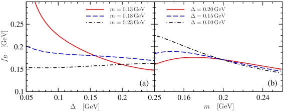
Figure 3: The decay constant $f_{B}$ in dependence on $m$ and $\Delta$. The condensates are taken to be ${\langle}\,\overline{q}q\,{\rangle}=(-0.27\,{\rm GeV})^{3}$ and ${\langle}\frac{\alpha_{s}}{\pi}G^{2}{\rangle}=(0.32\,{\rm GeV})^{4}$.

The gluon condensate may be related to the matrix element of the chromomagnetic interaction [2]:

$$3\lambda_{2}\,=\,\mu_{G}^{2}(H)=\frac{C_{\text{M}}(\mu)}{2M_{H}}{\langle}H|\bar{Q_{v}}\frac{1}{2}\sigma\cdot GQ_{v}|H{\rangle}\,=\,\frac{3}{2}m_{Q}(M_{H^{*}}-M_{H})\;.$$ (37)

Such a link was used in [7], but we will not use it because it formally belongs to $1/m_{Q}$ corrections, which are not considered here. Also, it turns out that such a choice doesn’t lead to any dramatic differences, when numerical results in $\Delta\to 0$ limit are compared to those from [7].

Within the full theory (Standard Model) at quark level, the weak current is

$$J_{f}^{\alpha}=\overline{q}_{f}\gamma^{\alpha}(1-\gamma_{5})Q\;,$$ (38)

where $Q$ is the heavy quark field in the full theory. Within HQEFT this current will, below the renormalization scale $\mu=m_{Q}\,(=m_{b},m_{c})$, be modified in the following way [2]:

$$J_{f}^{\alpha}={\overline{\chi}}_{a}\xi^{\dagger}_{af}\Gamma^{\alpha}Q_{v}\,+{\cal O}(m_{Q}^{-1})\;,$$ (39)

where

$$\Gamma^{\alpha}\;=\;C_{\gamma}\,\gamma^{\alpha}\,L\;+\,C_{v}\,v^{\alpha}\,R\;.$$ (40)

Figure 4: Diagrams for bosonization of the left handed quark current to leading order, determining $\alpha_{H}$

Bosonising this current by calculating diagrams from Fig. 4 we obtain to zeroth order in the axial field and to first order in the gluon condensate the weak current

$$J_{f}^{\alpha}=\frac{\alpha_{H}}{2}Tr\left[\xi^{\dagger}_{hf}\Gamma^{\alpha}H_{vh}\right]\;,$$ (41)

where heavy meson decay constant is given by

$$f_{H}=\frac{C_{\gamma}+C_{v}}{\sqrt{M_{H}}}\alpha_{H}\;,$$ (42)

with $C_{\gamma}=1.077$ and $C_{v}=0.0489$ being Wilson coefficients within HQEFT [2]. In addition $f_{B}$ and $f_{D}$ have chiral corrections of order 20 MeV (see [7] and references therein), as well as $1/m_{Q}$ corrections not considered here. From the diagrams in Fig. 4, we obtain:

$$\alpha_{H} =-2iG_{H}N_{c}\Big{\{}-I_{1}+(m-\Delta)I_{1,1}$$

$$\quad+\frac{m\pi^{2}}{N_{c}}\big{\langle}\frac{\alpha_{s}}{\pi}G^{2}\big{\rangle}\big{[}-mI_{4}+I_{3,1}+m(m-\Delta)I_{4,1}\big{]}\Big{\}}\;,$$ (43)

where divergent integrals $I_{1}$ and $I_{1,1}$ will be expressed in terms of model parameters. Since this is the only predicted quantity depending on $I_{1}$ it is easy to accommodate physical values of $f_{H}$, using (24) and adjusting the quark condensate, see Fig. 6(b). In the limit $\Delta\rightarrow 0$

$$\alpha_{H}\equiv-2iG_{H}N_{c}\left(-I_{1}+mI_{3/2}+\frac{i\,\kappa_{H}}{N_{c}\,m^{2}}{\langle}\frac{\alpha_{s}}{\pi}G^{2}{\rangle}\right)\;.$$ (44)

where $\kappa_{H}\,=\,(3\pi-4)/384$, in agreement with [7]. Furthermore, eliminating divergent integrals, one obtains

$$\alpha_{H}=\frac{G_{H}}{2}\left(-\frac{{\langle}\,\overline{q}q\,{\rangle}}{m}\,-\,\,\frac{m^{2}}{4\pi}\,+\,\frac{3(1-g_{A})}{2\rho}f_{\pi}^{2}\,-\,\frac{(3\pi-8))}{192m^{2}}{\langle}\frac{\alpha_{s}}{\pi}G^{2}{\rangle}\right)\;.$$ (45)

In the limit $\Delta\rightarrow m$

$$\alpha_{H}\equiv-2iG_{H}N_{c}\left(-I_{1}+\frac{i}{96N_{c}\,m^{2}}{\langle}\frac{\alpha_{s}}{\pi}G^{2}{\rangle}\right)\;,$$ (46)

or, eliminating divergent integrals,

$$\alpha_{H}=\frac{G_{H}}{2}\left(-\frac{{\langle}\,\overline{q}q\,{\rangle}}{m}-\frac{{\langle}\frac{\alpha_{s}}{\pi}G^{2}{\rangle}}{24m^{2}}\right)\;.$$ (47)

This completes the specification and bosonisation of the HL$\chi$QM. The remaining free parameters of the model are two condensates ${\langle}\,\overline{q}q\,{\rangle}$ and ${\langle}\frac{\alpha_{s}}{\pi}G^{2}{\rangle}$ and two constituent masses $m$ and $\Delta$. We can now apply the model to calculation of phenomenological quantities, starting with the Isgur-Wise function.

4 The Isgur-Wise function

Figure 5: Bosonisation corresponding to the Isgur-Wise function.

The Isgur-Wise function [1], $\xi(\omega)$, relates all the form factors describing the processes $B\to D(D^{*})$ in the heavy quark limit. In our framework it can be defined via bosonisation of heavy-heavy quark current responsible for $B\rightarrow D$ transition:

$$\overline{Q_{v_{b}}^{(+)}}\,\gamma^{\mu}\,LQ_{v_{c}}^{(+)}\;\longrightarrow\;-\xi(\omega)Tr\left[\overline{H_{c}^{(+)}}\gamma^{\mu}LH_{b}^{(+)}\right]\;\equiv\;J_{b\rightarrow c}^{\mu}\;\;.$$ (48)

Here $Q_{v_{c}}$ and $Q_{v_{c}}$ are the $c$ and $b$ quark fields within HQEFT. The IW function can be determined by calculating the diagrams shown in figure (5).

One normally expects that emission of the soft gluons from a heavy quark doesn’t occur at the zeroth order in $1/m_{Q}$. Namely, using the HQET Lagrangian (2), and differentiating the expressions involving heavy quark propagators according (11), will naturally, for diagrams of same class as those on Fig. 4, lead to expressions proportional to $v_{\mu}v_{\nu}G^{a}_{\mu\nu}=0$, where $v_{\mu}$ is either $v_{b}$ or $v_{c}$. However, for the Isgur-Wise function there are two velocities ($v_{b}$ and $v_{c}$) in play in the diagram. Therefore one may obtain contributions proportional to

$$v_{b}^{\mu}v_{c}^{\nu}G^{a}_{\mu\nu}\;\;,$$ (49)

which will generally, away from the strict heavy quark limit $\omega\rightarrow 1$, be different from zero. Let us also mention that some care is required because momentum flow in the diagrams for the translationally non-invariant amplitudes in the Fock-Schwinger gauge is non-trivial, see Fig. 5.

The corresponding results for diagrams (a)–(d) are

$$\xi(\omega)_{a} =iG_{H}^{2}N_{c}\left((m-\frac{2}{\omega+1}\Delta)I_{1,1,1}-\frac{2}{\omega+1}I_{1,1}\right)\;\,,$$ (50)

$$\xi(\omega)_{b} =iG_{H}^{2}{\langle}\frac{\alpha_{s}}{\pi}G^{2}{\rangle}m\pi^{2}\left(m^{2}I_{4,1,1}+I_{3,1,1}-\frac{2m}{\omega+1}\left(I_{4,1}+\Delta I_{4,1,1}\right)\right)\;\,,$$ (51)

$$\xi(\omega)_{c} =\frac{i}{12}G_{H}^{2}{\langle}\frac{\alpha_{s}}{\pi}G^{2}{\rangle}m\pi^{2}(\omega-1)I_{2,2,2}\;\,,$$ (52)

$$\xi(\omega)_{d} =\frac{i}{12}G_{H}^{2}\big{\langle}\frac{\alpha_{s}}{\pi}G^{2}\big{\rangle}\pi^{2}(\omega-1)\bigg{(}-I_{1,2,3}-I_{1,3,2}+\big{(}m(\omega+1)-2\Delta\big{)}I_{1,3,3}\bigg{)}\;\,.$$ (53)

Since loop integrals have at the least two heavy and one light quark propagator, integrals of the type $I_{n,r,s}$ occur above, and they are defined in the Appendix A. We find that the identity $\xi(\omega=1)=1$ follows from normalization of the vector current in eq. (18):

$$\xi(\omega=1)\,=\;\left(\xi_{a}\,+\,\xi_{b}+\xi_{c}\,+\,\xi_{d}\right)_{\omega=1}\;=\;\left(\xi_{a}\,+\,\xi_{b}\right)_{\omega=1}\;=\,1\;.$$ (54)

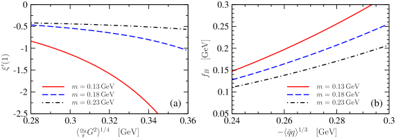
Figure 6: The slope of Isgur-Wise function $\xi^{\prime}(1)$ in dependence on the gluon condensate for various choices of the light quark constituent mass $m$ (a), and the decay constant $f_{B}$ in dependence on the quark condensate (b), for $\Delta=0.1\,{\rm GeV}$. Complementary plots are not so interesting because the dependence of $\xi^{\prime}(1)$ on the quark condensate and the dependence of $f_{B}$ on the gluon condensate are rather small.

Finally, for the slope of the IW function in the no-recoil limit $\omega\to 1$, we have

$$\xi^{\prime}(1)_{a} =iG_{H}^{2}N_{c}\left(\frac{1}{2}I_{1,1}-\big{(}\frac{1}{3}m-\frac{5}{6}\Delta\big{)}I_{1,2}-\frac{2}{3}\Delta(m-\Delta)\big{(}I_{1,3}-2m^{2}I_{3,1}\big{)}\right)\;\,,$$ (55)

$$\xi^{\prime}(1)_{b} =iG_{H}^{2}{\langle}\frac{\alpha_{s}}{\pi}G^{2}{\rangle}m\pi^{2}\left(\frac{1}{4}I_{2,4}+\frac{m}{6}(m-\Delta)I_{3,4}+\frac{m}{2}\big{(}I_{4,1}+\Delta I_{4,2}\big{)}\right)\;\,,$$ (56)

$$\xi^{\prime}(1)_{c} =iG_{H}^{2}{\langle}\frac{\alpha_{s}}{\pi}G^{2}{\rangle}\frac{m\pi^{2}}{12}I_{2,4}\;\,$$ (57)

$$\xi^{\prime}(1)_{d} =-iG_{H}^{2}{\langle}\frac{\alpha_{s}}{\pi}G^{2}{\rangle}\frac{\pi^{2}}{6}\bigg{(}I_{1,5}-(m-\Delta)I_{1,6}\bigg{)}\;\,.$$ (58)

All the $I_{n,r}$ integrals above can be evaluated using formulas from Appendix A.

5 Results and discussion

Numerical results are presented in Figs. 6 and 7. Fig. 6 displays the slope $\xi^{\prime}(1)$ of IW function as a function of the gluon condensate and the heavy meson decay constant $f_{B}$ as a function of the quark condensate, while Fig. 7 shows slope $\xi^{\prime}(1)$ for some generic condensate values in dependence on the dynamical masses $\Delta$ and $m$. One observes that for reasonable intervals of masses slope is of the order of -1 and beyond, which is in agreement with values mentioned in the Introduction, as well as with values obtained within other theoretical frameworks [31] and on the lattice [32].

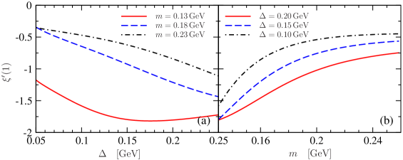
Figure 7: The slope of Isgur-Wise function $\xi^{\prime}(1)$ at no recoil point as a function of $\Delta$ for three values of $m$ (a), and as a function of $m$ for three values of $\Delta$ (b). The condensates are taken to be ${\langle}\,\overline{q}q\,{\rangle}=(-0.27\,{\rm GeV})^{3}$ and ${\langle}\frac{\alpha_{s}}{\pi}G^{2}{\rangle}=(0.32\,{\rm GeV})^{4}$.

It should be noticed that values for $\xi^{\prime}(1)$ of order or bigger than one prefer smaller constituent mass than in [7]. For easier overview of analytical results, as well as for their numerical checks, it is convenient to again investigate limit $\Delta\to m$. After using constant values for integrals in this limit, as given in Appendix A one obtains simple expression

$$\xi^{\prime}(1)=\frac{(3g_{{\cal A}}-1)}{4}-\frac{(1+3g_{{\cal A}})}{4f_{\pi}^{2}}\left\{\frac{m^{2}N_{c}}{2\pi^{2}}+\frac{11}{315m^{2}}{\langle}\frac{\alpha_{s}}{\pi}G^{2}{\rangle}\right\}\;.$$ (59)

Numerical values in this limit are not unreasonable.

In conclusion, we have presented an improved Heavy-Light Chiral Quark Model where introducing additional mass parameter in the heavy-quark propagator resulted in a flexible model capable of consistent description of heavy-meson decays, where we placed particular emphasis on a characterization of Isgur-Wise function. Further applications of the model, such as calculation of non-factorizable amplitudes for non-leptonic heavy-meson decays could now be attempted. As the slope of the IW function is steeper than the one used in, say, Ref. [18], the partial amplitudes for $B\rightarrow D\overline{D}$ depending on the IW function, might be overestimated there. This will then have consequences for the size of the overall amplitude.

Acknowledgement

K.K. is grateful for a warm hospitality of the Department of Physics at the University of Oslo. This work was supported by Research Council of Norway and the Croatian Ministry of Science, Education and Sport, contract no. 119-0982930-1016.

Appendix A Loop integrals

Three-, two-, and one-point loop integrals with one light-quark propagator occurring in the calculations are:

$$I_{n,r,s}^{\alpha\beta\cdots} =\int\frac{\textrm{d}^{4}p}{(2\pi)^{4}}\,\frac{p^{\alpha}p^{\beta}\cdots}{(p^{2}-m^{2}+i\epsilon)^{n}\,(p\cdot v-\Delta+i\epsilon)^{r}\,(p\cdot v^{\prime}-\Delta+i\epsilon)^{s}}\;,$$ (A1)

$$I_{n,r}^{\alpha\beta\cdots} =\int\frac{\textrm{d}^{4}p}{(2\pi)^{4}}\,\frac{p^{\alpha}p^{\beta}\cdots}{(p^{2}-m^{2}+i\epsilon)^{n}\,(p\cdot v-\Delta+i\epsilon)^{r}}\;,$$ (A2)

$$I_{n}^{\alpha\beta\cdots} =\int\frac{\textrm{d}^{4}p}{(2\pi)^{4}}\,\frac{p^{\alpha}p^{\beta}\cdots}{(p^{2}-m^{2}+i\epsilon)^{n}}\;.$$ (A3)

To evaluate such integrals one first reduces tensor to scalar ones using relations ($\omega\equiv v\cdot v^{\prime}$):

$$I^{\alpha}_{n,s} =(I_{n,s-1}+\Delta I_{n,s})v^{\alpha}\;\,,$$ (A4)

$$I^{\alpha\beta}_{n,1} =\frac{1}{3}\Big{[}I_{n-1,1}+m^{2}I_{n,1}-\Delta I_{n}-\Delta^{2}I_{n,1}\Big{]}g^{\alpha\beta}\;\,,$$

$$\quad-\frac{1}{3}\Big{[}I_{n-1,1}+m^{2}I_{n,1}-4\Delta I_{n}-4\Delta^{2}I_{n,1}\Big{]}v^{\alpha}v^{\beta}\;\,,$$ (A5)

$$I^{\alpha\beta\gamma}_{n,1} =\frac{1}{2}\Big{[}-I_{n-1}-(m^{2}-4\Delta^{2})I_{n}-2\Delta I_{n-1,1}-2\Delta(m^{2}-2\Delta^{2})I_{n,1}\Big{]}v^{\alpha}v^{\beta}v^{\gamma}\;\,,$$

$$\quad+\frac{1}{3}\Big{[}\frac{3}{4}I_{n-1}+\big{(}\frac{3}{4}m^{2}-\Delta^{2}\big{)}I_{n}+\Delta I_{n-1,1}$$

$$\qquad\qquad\qquad+\Delta(m^{2}-\Delta^{2})I_{n,1}\Big{]}(v^{\alpha}g^{\beta\gamma}+v^{\beta}g^{\alpha\gamma}+v^{\gamma}g^{\alpha\beta})$$ (A6)

$$I^{\alpha}_{n,r,s} =\frac{1}{\omega^{2}-1}\bigg{\{}(\omega I_{n,r,s-1}-I_{n,r-1,s})v^{\alpha}+(\omega I_{n,r-1,s}-I_{n,r,s-1})v^{\prime\alpha}\;\,,$$

$$\qquad\qquad\qquad+\Delta(\omega-1)I_{n,r,s}(v^{\alpha}+v^{\prime\alpha})\bigg{\}}\;\,.$$ (A7)

(Reduction of one-point $I_{n}^{\alpha\beta\cdots}$ tensor integrals is simple and well-known.) Now all scalar two-point integrals $I_{n,s}$ can be reduced to linear combinations of $I_{n,1}$ integrals using general recursion formula

$$I_{n,s}=\frac{-4n}{s^{2}-3s+2}\bigg{\{}(n+s-3)I_{n+1,s-2}+m^{2}(n+1)I_{n+2,s-2}\\ +\Delta\frac{s^{2}-3s+2}{s-1}I_{n+1,s-1}\bigg{\}}\;,$$ (A8)

valid for $s>2$, whereas the special case $s=2$ is

$$I_{n,2}=-2n\big{(}I_{n+1}+\Delta I_{n+1,1}\big{)}\;.$$ (A9)

For the calculation of the slope $\xi^{\prime}(1)$ of Isgur-Wise function, one additionally needs derivatives of three-point integrals at point $\omega=1$. Integrals themselves at this point are trivially given by

$$I_{n,r,s}(1)\;=\;I_{n,r+s}$$ (A10)

The derivatives are given by

$$\left.\frac{\partial I_{n,r,s}(\omega)}{\partial\omega}\right|_{\omega=1}=\frac{rs}{2(n-1)}I_{n-1,r+s+2}\qquad{\rm for}\quad n>1\;,$$ (A11)

while for $n=1$ we have special case:

$$\left.\frac{\partial I_{1,r,s}(\omega)}{\partial\omega}\right|_{\omega=1}=-\frac{rs}{r+s+1}\big{(}2\frac{r+s-1+\epsilon}{r+s}I_{1,r+s}+2\Delta I_{1,r+s+1}+\frac{2m^{2}}{r+s}I_{2,r+s}\big{)}\;,$$ (A12)

where dimensional regularization parameter $\epsilon$ is relevant only for divergent case $r=s=1$ where using $\lim_{\epsilon\to 0}\epsilon I_{1,2}=-i/(8\pi)$ one gets

$$\left.\frac{\partial I_{1,1,1}(\omega)}{\partial\omega}\right|_{\omega=1}=-\frac{1}{3}\big{(}I_{1,2}+2\Delta I_{1,3}-4\Delta m^{2}I_{3,1}\big{)}\;.$$ (A13)

Then again recursion formulas above above can be used to reduce everything to $I_{n,1}$ integrals. These integrals can be explicitly evaluated and they read

$$I_{n,1} \equiv\frac{i}{16\pi^{2}m^{2n-3}}\>a_{n}(\frac{\Delta}{m})\;,\qquad\text{where}$$ (A14)

$$a_{2}(x) =-\frac{1}{1-x^{2}}\mathcal{F}(x)\quad\xrightarrow{x\to 1}-2$$ (A15)

$$a_{3}(x) =\frac{1}{4}\frac{1}{(1-x^{2})^{2}}\left(\mathcal{F}(x)-2x+2x^{3}\right)\quad\xrightarrow{x\to 1}\frac{1}{3}$$ (A16)

$$a_{4}(x) =-\frac{1}{24}\frac{1}{(1-x^{2})^{3}}\left(3\mathcal{F}(x)-10x+14x^{3}-4x^{5}\right)\quad\xrightarrow{x\to 1}-\frac{2}{15}$$ (A17)

$$a_{5}(x) =\frac{1}{192}\frac{1}{(1-x^{2})^{4}}\left(15\mathcal{F}(x)-66x+118x^{3}-68x^{5}+16x^{7}\right)\quad\xrightarrow{x\to 1}\frac{1}{14}$$ (A18)

$$a_{6}(x) =-\frac{1}{1920}\frac{1}{(1-x^{2})^{5}}\left(105\mathcal{F}(x)-558x+1210x^{3}\right.$$

$$\qquad\qquad\qquad\qquad\qquad\left.-1052x^{5}+496x^{7}-96x^{9}\right)\quad\xrightarrow{x\to 1}-\frac{2}{45}\;.$$ (A19)

Here the function $\mathcal{F}(x)$ is [33]

$$\mathcal{F}(x) =\sqrt{x^{2}-1+i\epsilon}\Big{(}\log(x-\sqrt{x^{2}-1+i\epsilon})-\log(x+\sqrt{x^{2}-1+i\epsilon})\Big{)}$$ (A20)

Note that $\mathcal{F}(x)\xrightarrow{x\to 0}\pi$, which gives the various $a_{n}(0)$. Furthermore, $\mathcal{F}(x)=-2xF(1/x)$, where $F(1/x)$ is function from Eq. (A2) of [34].

This reduction of integrals is easy to implement on a computer and corresponding Mathematica code is available from the authors upon request.

References

-
[1]
N. Isgur and M. B. Wise,
Phys. Lett. B 232 (1989) 113,
N. Isgur and M. B. Wise, Phys. Lett. B 237 (1990) 527. - [2] M. Neubert, Phys. Rept. 245 (1994) 259 [arXiv:hep-ph/9306320].
- [3] W. A. Bardeen and C. T. Hill, Phys. Rev. D 49 (1994) 409 [arXiv:hep-ph/9304265].
- [4] D. Ebert, T. Feldmann, R. Friedrich and H. Reinhardt, Nucl. Phys. B 434 (1995) 619 [arXiv:hep-ph/9406220].
- [5] D. Ebert, T. Feldmann and H. Reinhardt, Phys. Lett. B 388 (1996) 154 [arXiv:hep-ph/9608223].
-
[6]
A. Deandrea, N. Di Bartolomeo, R. Gatto, G. Nardulli and A. D. Polosa,
Phys. Rev. D 58 (1998) 034004
[arXiv:hep-ph/9802308],
A. D. Polosa, Riv. Nuovo Cim. 23N11 (2000) 1 [arXiv:hep-ph/0004183]. - [7] A. Hiorth and J. O. Eeg, Phys. Rev. D 66 (2002) 074001 [arXiv:hep-ph/0206158].
- [8] A. Hiorth and J. O. Eeg, Eur. Phys. J. direct C 30 (2003) 006 [Eur. Phys. J. C 32S1 (2004) 69] [arXiv:hep-ph/0301118].
- [9] H. Hogaasen and M. Sadzikowski, Z. Phys. C 64 (1994) 427 [arXiv:hep-ph/9402279].
- [10] H. Y. Cheng, C. K. Chua and C. W. Hwang, Phys. Rev. D 69 (2004) 074025 [arXiv:hep-ph/0310359].
- [11] F. Jugeau, A. Le Yaouanc, L. Oliver and J. C. Raynal, arXiv:hep-ph/0604059.
- [12] J. D. Bjorken, talk at Les Rencontre de la Valle d’Aoste, La Thuile, Italy, Mar 18–24, 1990, SLAC-PUB-5278.
- [13] N. Uraltsev, Phys. Lett. B501 (2001) 86, [arXiv:hep-ph/0011124].
- [14] E. Barberio et al. [Heavy Flavor Averaging Group], arXiv:0808.1297 [hep-ex], and updates at http://www.slac.stanford.edu/xorg/hfag/.
-
[15]
S. Bertolini, J. O. Eeg and M. Fabbrichesi,
Nucl. Phys. B 449 (1995) 197
[arXiv:hep-ph/9409437],
V. Antonelli, S. Bertolini, J. O. Eeg, M. Fabbrichesi and E. I. Lashin, Nucl. Phys. B 469 (1996) 143 [arXiv:hep-ph/9511255],
S. Bertolini, J. O. Eeg and M. Fabbrichesi, Nucl. Phys. B 476 (1996) 225 [arXiv:hep-ph/9512356],
S. Bertolini, J. O. Eeg, M. Fabbrichesi and E. I. Lashin, Nucl. Phys. B 514 (1998) 63 [arXiv:hep-ph/9705244],
S. Bertolini, J. O. Eeg, M. Fabbrichesi and E. I. Lashin, Nucl. Phys. B 514 (1998) 93 [arXiv:hep-ph/9706260],
S. Bertolini, J. O. Eeg and M. Fabbrichesi, Phys. Rev. D 63 (2001) 056009 [arXiv:hep-ph/0002234],
- [16] J. O. Eeg, A. Hiorth and A. D. Polosa, Phys. Rev. D 65 (2002) 054030 [arXiv:hep-ph/0109201].
- [17] J. O. Eeg, S. Fajfer and J. Zupan, Phys. Rev. D 64 (2001) 034010 [arXiv:hep-ph/0101215].
- [18] J. O. Eeg, S. Fajfer and A. Prapotnik, Eur. Phys. J. C 42 (2005) 29 [arXiv:hep-ph/0501031].
- [19] J. A. Macdonald Sørensen and J. O. Eeg, Phys. Rev. D 75 (2007) 034015 [arXiv:hep-ph/0605078].
-
[20]
J. A. Cronin,
Phys. Rev. 161 (1967) 1483,
S. Weinberg, Physica A 96 (1979) 327,
D. Ebert and M. K. Volkov, Z. Phys. C 16 (1983) 205,
A. Manohar and H. Georgi, Nucl. Phys. B 234 (1984) 189,
J. Bijnens, H. Sonoda and M. B. Wise, Can. J. Phys. 64 (1986) 1,
D. Ebert and H. Reinhardt, Nucl. Phys. B 271 (1986) 188,
D. Diakonov, V. Y. Petrov and P. V. Pobylitsa, Nucl. Phys. B 306 (1988) 809,
D. Espriu, E. de Rafael and J. Taron, Nucl. Phys. B 345 (1990) 22 [Erratum-ibid. B 355 (1991) 278]. - [21] V. A. Novikov, M. A. Shifman, A. I. Vainshtein and V. I. Zakharov, Fortsch. Phys. 32 (1984) 585.
- [22] A. Pich and E. de Rafael, Nucl. Phys. B 358 (1991) 311.
-
[23]
J. O. Eeg and I. Picek,
Phys. Lett. B 301 (1993) 423,
J. O. Eeg and I. Picek, Phys. Lett. B 323 (1994) 193 [arXiv:hep-ph/9312320],
A. E. Bergan and J. O. Eeg, Phys. Lett. B 390 (1997) 420 [arXiv:hep-ph/9609262]. - [24] M. B. Wise, Phys. Rev. D 45 (1992) 2188.
- [25] R. Casalbuoni, A. Deandrea, N. Di Bartolomeo, R. Gatto, F. Feruglio and G. Nardulli, Phys. Rept. 281 (1997) 145 [arXiv:hep-ph/9605342].
- [26] M. B. Wise, arXiv:hep-ph/9306277.
- [27] B. Grinstein, arXiv:hep-ph/9508227.
- [28] C. G. Boyd and B. Grinstein, Nucl. Phys. B 442 (1995) 205 [arXiv:hep-ph/9402340].
- [29] I. W. Stewart, Nucl. Phys. B 529 (1998) 62 [arXiv:hep-ph/9803227].
- [30] E. E. Jenkins, Nucl. Phys. B 412 (1994) 181 [arXiv:hep-ph/9212295].
- [31] V. Morenas, A. Le Yaouanc, L. Oliver, O. Pene and J. C. Raynal, Phys. Rev. D 56 (1997) 5668 [arXiv:hep-ph/9706265].
- [32] K. C. Bowler, G. Douglas, R. D. Kenway, G. N. Lacagnina and C. M. Maynard [UKQCD Collaboration], Nucl. Phys. B 637 (2002) 293 [arXiv:hep-lat/0202029].
- [33] A. O. Bouzas, Eur. Phys. J. C 12 (2000) 643 [arXiv:hep-ph/9910536].
- [34] I. W. Stewart, Nucl. Phys. B 529 (1998) 62 [arXiv:hep-ph/9803227].