Study of the $f_{2}(1270)$, $f_{2}^{\prime}(1525)$, $f_{0}(1370)$ and $f_{0}(1710)$ in the $J/\psi$ radiative decays

Abstract

In this paper we present an approach to study the radiative decay modes of the $J/\psi$ into a photon and one of the tensor mesons $f_{2}(1270)$, $f^{\prime}_{2}(1525)$, as well as the scalar ones $f_{0}(1370)$ and $f_{0}(1710)$. Especially we compare predictions that emerge from a scheme where the states appear dynamically in the solution of vector meson–vector meson scattering amplitudes to those from a (admittedly naive) quark model. We provide evidence that it might be possible to distinguish amongst the two scenarios, once improved data are available.

I Introduction

Interactions amongst hadrons may be sufficiently strong to produce bound states — this picture even emerges naturally when starting from a quark model extraordinary . Famous examples of those are nuclei, but also amongst mesons a large number of states were recently identified as candidates for hadronic molecules. However, only if one channel is largely dominant and the (quasi)–bound–state poles are located close to the corresponding continuum threshold for the constituents that form the molecule through an $s$–wave interaction evidence ; Weinberg:1962hj or if the $N_{c}$ behavior of the system can be controlled rios , a model independent access to the nature of the state appears to be possible. On the other hand there is a large number of proposed molecular states, where neither of the mentioned criteria applies. In this case it needs to be demonstrated that the molecular picture describes the properties of the states better than, say, a conventional quark–model description. This might emerge, e.g., since the pattern of SU(3)–flavor breaking turns out to be different for hadron–hadron states, due to the different analytic structure of their scattering amplitudes. In this paper we discuss observables that might qualify for such a test for the possible molecular nature of the $f_{2}(1270)$, $f^{\prime}_{2}(1525)$, $f_{0}(1710)$, and $f_{0}(1370)$.

The reactions we will focus on are decays of the $J/\psi$. The decays of $J/\psi$ into a vector meson $\phi$ or $\omega$ and two pseudoscalars, including their non-perturbative final state interactions driven by the presence of the scalar mesons $f_{0}(600)$ and $f_{0}(980)$, were studied recently in Refs. ulfjose ; palochiang ; lahde . These processes proceed through an OZI violating strong interaction and it was assumed that the transition $J/\psi\to V$ provides a scalar source term allowing for an investigation of scalar form factors (for corrections induced by the interaction of the pseudoscalars with the vector meson see Refs. palochiang ; liu ).

Analogous to the decay modes mentioned above are the modes $J/\psi\to\phi(\omega)f_{2}(1270)$, $J/\psi\to\phi(\omega)f^{\prime}_{2}(1525)$ and $J/\psi\to K^{*0}(890)\bar{K}^{*0}_{2}(1430)$. These decays were recently studied in Ref. albertozou following similar steps as done in Refs. ulfjose ; palochiang ; lahde , within the scheme where these tensor states are dynamically generated from the interaction of pairs of vector mesons. Indeed, in Ref. raquel it was shown that the $f_{2}(1270)$ and $f_{0}(1370)$ states appear naturally as bound states of $\rho\rho$ using the interaction kernel provided by the hidden gauge Lagrangians hidden1 ; hidden2 ; hidden3 ; ulfvec . An extension to SU(3) of the former work of Ref. raquel done in Ref. gengvec ; Geng:2009gb , studying the interaction of pairs of vectors, shows that there are as many as 11 states dynamically generated, some of which can be associated to known resonances, namely the $f_{2}(1270),f^{\prime}_{2}(1525)$ and $K^{*}_{2}(1430)$ resonances, as well as the $f_{0}(1370)$ and $f_{0}(1710)$. In this paper we investigate the same $J/\psi$ decays together with their radiative counterparts and make predictions for ratios of decay rates for the mentioned molecular picture and a naive quark model assignment.

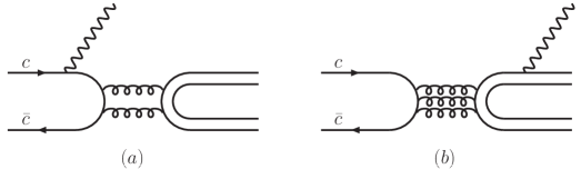
Figure 1: Two mechanisms of the $J/\psi$ radiative decays.

II Decay rates in the molecular picture

Two topologies are possible for the radiative decays of the $J/\psi$ into light hadrons, as shown in Fig. 1. Since the photon carries both an isospin 1 and an isospin 0 component, the hadronic final state for the mechanism of diagram $(b)$ can have an admixture of both isospins. In diagram $(a)$, on the other hand, also after the photon emission, the isospin of the $\bar{c}c$ pair is still zero and correspondingly the isospin of the hadronic final state is zero. Since at the charm quark mass $\alpha_{s}$ is about $1/3$, relatively small, and diagram $(b)$ involves an additional loop, diagram $(a)$ is expected to be the dominant process physrep and we therefore may assume the radiative $J/\psi$ decays as a source for isoscalar light hadrons. This is also confirmed by data Amsler:2008zzb . More than this, under the dominance of diagram (a), the state after the radiation is still a $c\bar{c}$ and hence an SU(3) singlet, which is relevant for the present study.

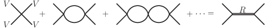
Figure 2: Schematic representation of dynamically generated resonances from vector meson-vector meson interaction.

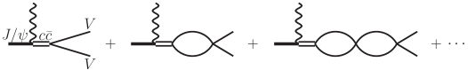
Figure 3: Schematic representation of $J/\psi$ decay into a photon and one dynamically generated resonance.

We now need to calculate the formation of the resonances. This calculation depends on the assumed nature of the states. In this section we will discuss the rates that emerge in a molecular picture for the mentioned resonances — namely they are assumed to emerge from the non-perturbative interactions of vector mesons amongst themselves. We readily get the SU(3) singlet combination of two vectors from

$$\mathrm{VV}_{\mbox{SU(3) singlet}}=\mathrm{Tr}[V.V],$$ (1)

where $V$ is the SU(3) matrix of the vector mesons

$$V=\left(\begin{array}[]{ccc}\frac{1}{\sqrt{2}}\rho^{0}+\frac{1}{\sqrt{2}}\omega&\rho^{+}&K^{*+}\\ \rho^{-}&-\frac{1}{\sqrt{2}}\rho^{0}+\frac{1}{\sqrt{2}}\omega&K^{*0}\\ K^{*-}&\bar{K}^{*0}&\phi\end{array}\right).$$ (2)

We, thus, find the vertex

$$\mathrm{VV}_{\mbox{SU(3) singlet}}=\rho^{0}\rho^{0}+\rho^{+}\rho^{-}+\rho^{-}\rho^{+}+\omega\omega+K^{*+}K^{*-}+K^{*0}\bar{K}^{*0}+K^{*-}K^{*+}+\bar{K}^{*0}K^{*0}+\phi\phi.$$ (3)

One then projects this combination over the VV states which are the building blocks of the resonance produced, with unitary normalization (an extra factor $1/\sqrt{2}$ for identical particles or symmetrized ones) and phase convention $|\rho^{+}\rangle=-|1,+1\rangle$, $|K^{*-}\rangle=-|1/2,-1/2\rangle$ of isospin,

$$|\rho\rho\rangle_{\mathrm{I=0}} = -\frac{1}{\sqrt{6}}|\rho^{0}\rho^{0}+\rho^{+}\rho^{-}+\rho^{-}\rho^{+}\rangle,$$ (4)

$$|K^{*}\bar{K}^{*}\rangle_{\mathrm{I=0}} = -\frac{1}{2\sqrt{2}}|K^{*+}K^{*-}+K^{*0}\bar{K}^{*0}+K^{*-}K^{*+}+\bar{K}^{*0}K^{*0}\rangle,$$ (5)

$$|\omega\omega\rangle_{\mathrm{I=0}} = \frac{1}{\sqrt{2}}|\omega\omega\rangle,$$ (6)

$$|\phi\phi\rangle_{\mathrm{I=0}} = \frac{1}{\sqrt{2}}|\phi\phi\rangle,$$ (7)

and one gets the weights for primary VV production of the process $J/\psi\rightarrow\gamma\mathrm{VV}$:

$$w_{i}=\left\{\begin{array}[]{ll}-\sqrt{\frac{3}{2}}&\quad\mbox{for $\rho\rho$}\\ -\sqrt{2}&\quad\mbox{for $K^{*}\bar{K}^{*}$}\\ \frac{1}{\sqrt{2}}&\quad\mbox{for $\omega\omega$}\\ \frac{1}{\sqrt{2}}&\quad\mbox{for $\phi\phi$}\end{array}\right..$$ (8)

Note that these weights are just SU(3) symmetry coefficients, and they are obtained with the momentum-independent approximation of the production vertices, which is valid since the mass differences among the vector mesons are small.

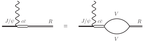
Figure 4: Schematic representation of $J/\psi$ decay into a photon and one dynamically generated resonance.

The next step consists in producing dynamically the resonance R which is shown diagrammatically in Fig. 2. Then in the $J/\psi\rightarrow\gamma\mathrm{VV}$ decay we naturally have a process as shown in Fig. 3 such that the part of the $J/\psi\rightarrow\gamma\mathrm{R}$ amplitude is then given by the process shown in Fig. 4, where the VV loop stands for the VV propagator, or $G$ function, which appears in the scattering amplitude for two vectors

$$T=(1-\tilde{V}G)^{-1}\tilde{V}$$ (9)

with $\tilde{V}$ the VV potential. In Fig. 4 one also has the couplings, $g_{j}$, of the resonance R to the different VV intermediate states, which are calculated and tabulated in Ref. gengvec ; Geng:2009gb . Altogether the amplitude for $J/\psi\rightarrow\gamma\mathrm{R}$ is proportional to

$$t_{J/\psi\rightarrow\gamma\mathrm{R}}\propto\sum_{j}w_{j}G_{j}g_{j}\ .$$ (10)

The resonance decay vertices do not appear in this expression, since they are irrelevant for the discussion below, which focuses on inclusive observables. In Table I the values for the $G_{j}$ and $g_{j}$ at the resonance peak obtained in Ref. gengvec ; Geng:2009gb are given. Note that the main component of the $f_{2}(1270)$ and $f_{0}(1370)$ ($f_{2}^{\prime}(1525)$ and $f_{0}(1710)$) is the $\rho\rho$ ($K^{*}{\bar{K}}^{*}$) pair, and the interference between the $\rho\rho$ and $K^{*}{\bar{K}}^{*}$ is constructive (destructive) for the $f_{2}(1270)$ and $f_{0}(1370)$ ($f_{2}^{\prime}(1525)$ and $f_{0}(1710)$).

Table 1: $G_{j}$’s and $g_{j}$’s appearing in Eq. (10), with $j$ one of the coupled channels: $\rho\rho$, $K^{*}\bar{K}^{*}$, $\omega\omega$, and $\phi\phi$. The $G_{j}$’s are in units of $10^{-3}$, and the $g_{j}$’s are in units of MeV.

R	$\rho\rho$		$K^{*}\bar{K}^{*}$		$\omega\omega$		$\phi\phi$
	$G$	$g$	$G$	$g$	$G$	$g$	$G$	$g$
$f_{2}(1270)$	$-4.37$	$10889$	$-2.34$	$4733$	$-4.97$	$-440$	$0.47$	$-675$
$f^{\prime}_{2}(1525)$	$-8.33$	$-2443$	$-4.27$	$10121$	$-9.62$	$-2709$	$-0.71$	$-4615$
$f_{0}(1370)$	$-8.09$	$7920$	$-4.14$	$1208$	$-9.11$	$-39$	$-0.63$	$12$
$f_{0}(1710)$	$-10.02$	$-1030$	$-7.81$	$7124$	$-11.15$	$-1763$	$-2.17$	$-2493$

Table 2: Ratios of $R_{T}=\Gamma_{\mathrm{J/\psi\rightarrow\gamma f_{2}(1270)}}/\Gamma_{J/\psi\rightarrow\gamma f^{\prime}_{2}(1525)}$ and $R_{S}=\Gamma_{J/\psi\rightarrow\gamma f_{0}(1370)}/\Gamma_{J/\psi\rightarrow\gamma f_{0}(1710)}$ within the molecular model and the quark model in comparison with data Amsler:2008zzb .

	Molecular picture	Quark model	Data
$R_{T}$	$2\pm 1$	$2.2$	$3.18^{+0.58}_{-0.64}$
$R_{S}$	$1.2\pm 0.3$	$2.2-2.5$
$R_{S}/R_{T}$	$0.6\pm 0.1$	$1-1.1$

For inclusive resonance production the partial decay widths are given by

$$\Gamma=\frac{1}{8\pi}\frac{1}{M_{J/\psi}^{2}}|t|^{2}q$$ (11)

where $q$ is the photon momentum in the $J/\psi$ rest system. For simplicity we here assume that the final phase space can be calculated with the nominal resonance mass. A more refined study would call for a proper folding with the resonance mass distribution (recall that this folding for the intermediate VV states is already done in Ref. gengvec ; Geng:2009gb ). While this is relevant when one has decays close to the threshold of the final state, in the present case there is plenty of phase space for the $J/\psi\rightarrow\gamma\mathrm{R}$ decay and the folding barely changes the results calculated at the central value of the resonance mass distribution.

The most difficult part of this study is the determination of the uncertainties. Since there is no proper effective field theory underlying this study, we need to estimate the uncertainties of the model via the uncertainties of the input quantities. The model used has 5 subtraction constants as parameters in the strangeness-zero channels gengvec ; Geng:2009gb . They were all demanded to take natural values, however, two of them were tuned a bit to get the masses of the tensor–mesons in agreement with data. In order to determine the uncertainties of the result we now vary all parameters independently: we produced a large number of results emerging from calculations with different subtraction constants under the constraint that the masses of the tensor mesons still are reproduced. In addition the vector coupling constant was varied within its 10 % uncertainty. From this study a 95 % confidence level could be determined. The corresponding results that we get within the molecular picture are shown in the first column in Table II and compared with the experimental data when available Amsler:2008zzb . Please note that the uncertainty of the super–ratio $R_{S}/R_{T}$ is considerably lower, since the uncertainties in $R_{S}$ and $R_{T}$ are correlated.

We can see that we obtain a band of values perfectly compatible with the experimental data for the ratio of rates of $J/\psi$ to $\gamma f_{2}(1270)$ and $\gamma f^{\prime}_{2}(1525)$. We get a central value of 2 for this ratio. As we will show below, the quark model prediction for this quantity, assuming that the resonances belong to the same flavor nonet, is similar.

In addition to the tensor channel the model also makes predictions for the ratio of the decay rates to the two scalar states $f_{0}(1370)$ and $f_{0}(1710)$, which are also dynamically generated in the approach of Ref. gengvec ; Geng:2009gb . The central value obtained is about 1.2 for the ratio of the decay rates to $\gamma f_{0}(1370)$ and $\gamma f_{0}(1710)$. One can trace this smaller value now, with respect to the case of the tensors, to a less efficient cancellation between $K^{*}\bar{K}^{*}$ and $\rho\rho$ in the case of the $f_{0}(1710)$ compared to the $f_{2}^{\prime}(1525)$, where the $\rho\rho$ coupling has also opposite sign to that of $K^{*}\bar{K}^{*}$. The SU(3) flavor content of the tensor and scalar resonances is similar within the model employed: $f_{0}(1370)$ and $f_{2}(1270)$ are mostly $\rho\rho$ molecules, while $f_{0}(1710)$ and $f^{\prime}_{2}(1525)$ are mostly $K^{*}\bar{K}^{*}$ molecules. Yet, the nontrivial dynamics of the coupled channels and the potentials $\tilde{V}$ of the hidden-gauge approach tend to produce a factor of two difference in the ratios of the decay rates of $J/\psi$ into states with similar flavor contents, although the uncertainties between the two ratios still overlap.

However, since the uncertainty of the super-ratio $R_{S}/R_{T}$ is smaller, the difference between 0.6 in the case of the molecular picture and the value around unity in the quark model picture to be discussed below, within their uncertainties, are quite distinct. Certainly the measurement of the ratio of decays to the scalar mesons should be a valuable piece of information to further test the nature of the resonances under consideration.

In the case of scalar mesons the intermediate pseudoscalar pairs (they are in L=0 for the scalar mesons) in the sum of Eq. (10) could provide some contribution. We find the most extreme case for the $f_{0}(1370)$, where the combination of $G_{j}g_{j}$ of Eq. (10) for $\pi\pi$ might be of the same order of magnitude as for the $\rho\rho$ component, however, almost purely imaginary, so that there is no interference with the $\rho\rho$ contribution. One must then rely upon the weighs $w_{j}$ to decide the relative size of the $\pi\pi$ and $\rho\rho$ contribution. The limited information from the PDG (see rates $\Gamma_{135}$, $\Gamma_{148}$, $\Gamma_{171}$) indicate that the rates for $J/\psi\rightarrow\gamma\rho\rho$ might be about one order of magnitude larger than for $J/\psi\rightarrow\gamma\pi\pi$  Amsler:2008zzb , so one can induce a smaller contribution of intermediate pions, but this limited experimental information should translate into larger uncertainties in the $R_{S}$ ratio of Table 2, of the order of an additional 10-20 %.

Please note that for the decay modes $J/\psi\to\phi(\omega)f_{2}(1270)$, $J/\psi\to\phi(\omega)f^{\prime}_{2}(1525)$ and $J/\psi\to K^{*0}(890)\bar{K}^{*0}_{2}(1430)$, estimated within the same molecular picture as used in this section, a good agreement with the data was achieved albertozou — see Fig. 6. In the next section we shall discuss the corresponding predictions for all the channels mentioned within an admittedly naive quark model.

III Flavor counting considerations

It is worth mentioning that the ratio of rates, $R_{T}$, obtained in Table II is related to the dominance of the strange components in $f^{\prime}_{2}(1525)$ and the nonstrange ones in $f_{2}(1270)$. In a simple $q\bar{q}$ model for these states one assumes that they belong to a nonet of tensor mesons, which includes the $K^{*}_{2}(1430)$ physrep . Certainly, in a quark model mixing between the SU(3) singlet $(u\bar{u}+d\bar{d}+s\bar{s})/\sqrt{3}$ and SU(3) octet isoscalar $(u\bar{u}+d\bar{d}-2s\bar{s})/\sqrt{6}$ is allowed. Since the mass difference between the $f_{2}(1270)$ and the $f_{2}^{\prime}(1525)$ is approximately the same as that between the $\omega$ and the $\phi$, we may assume ideal mixing between them, i.e., the $f_{2}(1270)$ corresponds to $(u\bar{u}+d\bar{d})/\sqrt{2}$, the $f_{2}^{\prime}(1525)$ to $s\bar{s}$ (see footnote ). The SU(3) singlet combination is now given by

$$S\sim u\bar{u}+d\bar{d}+s\bar{s}=\sqrt{2}\frac{1}{\sqrt{2}}{(u\bar{u}+d\bar{d})}+s\bar{s},$$ (12)

which provides a branching ratio

$$\frac{B_{J/\psi\rightarrow\gamma f_{2}(1270)}}{B_{J/\psi\rightarrow\gamma f^{\prime}_{2}(1525)}}=\left(\frac{\sqrt{2}}{1}\right)^{2}\frac{q_{2}}{q^{\prime}_{2}}\approx 2.2,$$ (13)

where $q_{2}$ and $q^{\prime}_{2}$ are the momenta of the $f_{2}(1270)$ and $f^{\prime}_{2}(1525)$ in the $J/\psi$ rest frame. This number is comparable to the one obtained in the molecular model discussed in the previous section, where the $f_{2}(1270)$ is mostly $\rho\rho$ and the $f^{\prime}_{2}(1525)$ is mostly $K^{*}\bar{K}^{*}$. A fully dynamical quark model calculation for the mentioned transitions, e.g. along the lines of Refs. Barnes:1996ff ; Barnes:2002mu , where the strong decays of the $f_{2}(1270)$ and the $f_{2}^{\prime}(1525)$ are well-described in the ${}^{3}P_{0}$ quark model, would be most welcome.

Analogous flavor counting arguments provide values between 2.2 and 2.5 for the ratio $R_{S}$ of Table II, depending on the masses used for the scalar states, which is considerably higher than the value found within the molecular model.

There are similar transitions that can be studied within the same framework, namely the ratios between the $J/\psi$ decays into $\phi(\omega)f_{2}(1270)$, $\phi(\omega)f^{\prime}_{2}(1525)$, $K^{*0}\bar{K}^{*0}_{2}(1430)$. Within the molecular model of the previous section those were studied in Ref. albertozou — the results of that reference, which describe the data well, although with a sizable uncertainty, are indicated in Fig. 6 as the blue shaded bands. It is straightforward to estimate the same ratios also within the simple quark model outlined above. Using the formulas obtained in Table I of Ref. albertozou for the production of the $s\bar{s}$, $\frac{1}{\sqrt{2}}(u\bar{u}+d\bar{d})$, and $s\bar{d}$ components, together with $\phi$, $\omega$ or $K^{*0}$, one immediately finds

$$R_{1} = \frac{\Gamma_{J/\psi\rightarrow\phi f_{2}(1270)}}{\Gamma_{J/\psi\rightarrow\phi f^{\prime}_{2}(1525)}}=2\left(\frac{\nu-1}{\nu+2}\right)^{2}\frac{q_{2}(\phi)}{q^{\prime}_{2}(\phi)},$$ (14)

$$R_{2} = \frac{\Gamma_{J/\psi\rightarrow\omega f_{2}(1270)}}{\Gamma_{J/\psi\rightarrow\omega f^{\prime}_{2}(1525)}}=\frac{1}{2}\left(\frac{2\nu+1}{\nu-1}\right)^{2}\frac{q_{2}(\omega)}{q^{\prime}_{2}(\omega)},$$ (15)

$$R_{3} = \frac{\Gamma_{J/\psi\rightarrow\omega f_{2}(1270)}}{\Gamma_{J/\psi\rightarrow\phi f_{2}(1270)}}=\frac{1}{2}\left(\frac{2\nu+1}{\nu-1}\right)^{2}\frac{q_{2}(\omega)}{q_{2}(\phi)},$$ (16)

$$R_{4} = \frac{\Gamma_{J/\psi\rightarrow K^{*0}\bar{K}^{*0}(1430)}}{\Gamma_{J/\psi\rightarrow\omega f_{2}(1270)}}=\left(\frac{3}{2\nu+1}\right)^{2}\frac{q_{2}(K^{*0})}{q_{2}(\omega)},$$ (17)

where the $q_{2}(\mathrm{M})$’s and $q^{\prime}_{2}(\mathrm{M})$’s are the momentum of the meson M in the $J/\psi$ rest frame in the corresponding decays, and $\nu$ measures the ratio of amplitudes for producing simultaneously two singlets and two octets of SU(3) in the $J/\psi$ decay into $\phi$ ($\omega$) albertozou .

Before comparing the resulting ratios to the data it is useful to estimate the allowed range for $\nu$. For that purpose we may switch to the quantity $\lambda_{\phi}$ defined in Ref. ulfjose , which is a measure of a subdominant component in the $J/\psi$ decay to $\phi$ and a pair of $q\bar{q}$ prior to hadronization as defined by

$$J/\psi\rightarrow\phi[s\bar{s}+\lambda_{\phi}\frac{1}{\sqrt{2}}(u\bar{u}+d\bar{d})]\rightarrow\phi MM,$$ (18)

and given in terms of $\nu$ by

$$\lambda_{\phi}=\sqrt{2}\left(\frac{\nu-1}{\nu+2}\right)\ .$$ (19)

Figure 5: $J/\psi$ decays into $\phi+q\bar{q}$ with one-OZI suppression (a) and double-OZI suppression (b).

One can estimate the natural value of the OZI violation parameter $\lambda_{\phi}$ using $N_{c}$ counting, with $N_{c}$ being the number of colors. In Fig. 5, we show the mechanisms of the $J/\psi$ decays into $\phi+q\bar{q}$ with single-OZI suppression and double-OZI suppression, as shown by (a) and (b), respectively. Taking into account that the strong coupling constant $g_{s}$ behaves as $1/\sqrt{N_{c}}$, and counting the closed loops by changing the gluon lines to double lines, one can see that diagram (a) counts as $N_{c}^{0}$, and (b) counts as $1/N_{c}$. Hence the double-OZI suppression mechanism shown in (b) is suppressed by a factor of $1/N_{c}$ compared with the single-OZI mechanism (a). Taking $N_{c}=3$, we get $\lambda_{\phi}\sim 0.33$. Correspondingly, $\nu\approx 1.9$. Note that this number provides only a crude estimate, and the value $\nu=1.45$, found in Ref. albertozou , as well as those used in Ref. ulfjose are roughly consistent with this estimate.

Experimentally one finds a band of values for each ratio: $R_{1}\approx 0.22-0.47$, $R_{2}\approx 12.33-49.00$, $R_{3}\approx 11.21-23.08$, and $R_{4}\approx 0.55-0.89$ albertozou . In Fig. 6, as the black solid line, the predictions from the naive quark model for the ratios are shown as a function of $\nu$ in the parameter range allowed. Also shown in the figure are the experimental data (gray shaded bands) as well as the predictions of Ref. albertozou (blue shaded bands). As can be seen from the figure, while the molecular model appears to be fully consistent with the data, there is no value for $\nu$ in the range allowed that brings all ratios in agreement with the data — however, for $\nu=1.7$ or larger, $R_{2}$ and $R_{3}$ agree with the data, while $R_{1}$ and $R_{4}$ are off only by two sigma, which one might still view as acceptable given the crudeness of the quark model used here. The important message of Fig. 6 is that the predictions of the molecular model discussed here and the naive quark model are quite distinct. Further experimental and theoretical analyses are necessary to really test the nature of these resonances using the processes studied here.

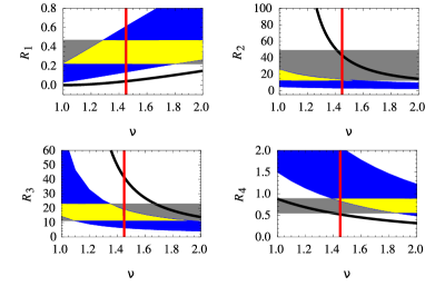
Figure 6: (Color on line) Comparison with data (gray shaded bands) of $R_{1}$, $R_{2}$, $R_{3}$, and $R_{4}$ calculated with Eqs. (14-17) within the quark model (solid black lines). The vertical solid red lines indicate $\nu=1.45$ obtained in Ref. albertozou . The results for the ratios of that reference, obtained using the molecular model, are shown by the blue shaded bands. The yellow regions indicate the overlap of the results of the molecular model with the data.

IV Further discussions

As can be seen from the numbers listed in Table 2, the central value of $R_{T}$ in the molecular model is similar to that in the quark model. However, they come from quite different physical sources. In the quark model, $R_{T}\approx 2.2$ comes mainly from the SU(3) flavor wave functions of the two tensor mesons modulo small kinematic correction as seen from Eq. (13). In the molecular model, the result about 2 comes from the nontrivial interference pattern between the dominant channel and the others. To be explicit, using the values of $G_{i}$ and $g_{i}$ given in Table 1 and $w_{i}$ given in Eq. (8), one gets $t_{o}/t_{d}=0.29$ for the $f_{2}(1270)$ and $t_{o}/t_{d}=-0.07$ for the $f_{2}^{\prime}(1525)$, where $t_{d}$ and $t_{o}$ denote the decay amplitudes from the dominant component and the other components, respectively. Note that $\left(\frac{t_{d}[f_{2}(1270)]}{t_{d}[f^{\prime}_{2}(1525)]}\right)^{2}\approx 0.9$ and $(1.29/0.93)^{2}\approx 2$. Contrary to the case of the tensor mesons, in the molecular model, the amplitude from the dominant component only gets a small correction from non-trivial interference with the other components for both the $f_{0}(1370)$ and the $f_{0}(1710)$. Moreover, the corrections for these two scalars are similar, $t_{o}/t_{d}$ is 9% for the $f_{0}(1370)$, and 6% for the $f_{0}(1710)$ (using the numbers given in Table 1). As a result, the value of $R_{S}$ is approximately 1 in the molecular model, which differs from that in the quark model.

We must mention that the current version of the PDG review Amsler:2008zzb quotes the observation of the $f_{0}(1710)$ in three $J/\psi$ radiative decay modes, i.e., $J/\psi\rightarrow\gamma f_{0}(1710)\rightarrow\gamma K\bar{K}$, $J/\psi\rightarrow\gamma f_{0}(1710)\rightarrow\gamma\omega\omega$, and $J/\psi\rightarrow\gamma f_{0}(1710)\rightarrow\gamma\pi\pi$, while no clear $f_{0}(1370)$ has been seen in these data. This, at first sight, seems to contradict the results in both the molecular model ($R_{S}=1.2\pm 0.3$) and the quark model ($R_{S}\approx 2.2-2.5$). However, this might be a consequence of the decay channels experimentally studied. For instance, in the molecular model used here the $f_{0}(1370)$ couples only very weakly to both $K\bar{K}$ and $\omega\omega$. Thus, the non-observation of this state in the $\gamma K\bar{K}$ and $\gamma\omega\omega$ decay modes of the $J/\psi$ decays should be of no surprise in that model. On the other hand, since in that model the $f_{0}(1370)$ couples much more strongly to $\pi\pi$ than the $f_{0}(1710)$ does, it seems mysterious that in the $J/\psi\rightarrow\gamma\pi\pi$ data Ablikim:2006db only the $f_{0}(1710)$ is seen but not the $f_{0}(1370)$. A possible explanation is that the scalar state peaking at $1765^{+4}_{-3}\pm 13$ MeV with a width of $145\pm 8\pm 69$ MeV Ablikim:2006db might not be the same as the $f_{0}(1710)$ observed in the $J/\psi\rightarrow\omega\pi\pi(K\bar{K})$. This conjecture is supported by the fact that the $f_{0}(1710)$ branching fractions to $\pi\pi$ and $K\bar{K}$ obtained from $J/\psi\rightarrow\gamma\pi\pi(K\bar{K})$ data Ablikim:2006db ; Bai:2003ww and $J/\psi\rightarrow\omega\pi\pi(K\bar{K})$ data Ablikim:2004qna ; Ablikim:2004st , $0.41^{+0.11}_{-0.17}$ and $<0.11$ at 95% confidence level, respectively, are not consistent with each other, which indicates that the states observed in these two sets of data might indeed be different. On the other hand, the $f_{0}(1710)$ in the molecular picture has a branching ratio $\Gamma_{\pi\pi}/\Gamma_{K\bar{K}}$ at a few percentage level gengvec ; Geng:2009gb , consistent with the $f_{0}(1710)$ observed in $J/\psi\rightarrow\omega\pi\pi(K\bar{K})$ Ablikim:2004qna ; Ablikim:2004st .

The new analysis of the BES II $J/\psi\rightarrow\gamma(\pi\pi\pi\pi)$ data Bugg:2009ch , which updates the analyses of the Mark III Bugg:1995jq and BES data Bai:1999mm , claims that the scalar state around $1.7\sim 1.8$ GeV is the $f_{0}(1790)$, which is also seen in $J/\psi\rightarrow\phi\pi\pi$ Ablikim:2004wn . The $f_{0}(1370)$ is also definitely needed to fit the data, while no $f_{0}(1710)$ is necessary. The observations are consistent with the molecular picture for the $f_{0}(1710)$ and $f_{0}(1370)$. Indeed, since in the molecular model the ratio $R_{S}=\frac{\Gamma_{J/\psi\rightarrow\gamma f_{0}(1370)}}{\Gamma_{J/\psi\rightarrow\gamma f_{0}(1710)}}$ is about 1 and the $f_{0}(1370)$ couples more strongly to $\rho\rho$ than the $f_{0}(1710)$ does, one would naively expect to see more $f_{0}(1370)$ than $f_{0}(1710)$ in $J/\psi\rightarrow\gamma(\pi\pi\pi\pi)$.

The study of scalar mesons between 1 and 2 GeV has always been complicated by possible mixing with nearby glueballs, see e.g. Ref. Close:2005vf and references therein. Things might become more subtle if there exists an extra scalar state, the $f_{0}(1790)$, in addition to the $f_{0}(1370)$, $f_{0}(1500)$, and $f_{0}(1710)$. In the molecular picture of Ref. gengvec ; Geng:2009gb , possible mixing of glueballs with the $f_{0}(1370)$ and $f_{0}(1710)$ is not considered, which is in line with the study of Ref. Close:2005vf . In that paper, it is suggested that the $f_{0}(1500)$ has a large glueball component while the $f_{0}(1370)$ and $f_{0}(1710)$ have relatively small glueball components. Certainly, one should keep in mind that the $f_{0}(1370)$ and $f_{0}(1710)$ in the molecular model are dynamically generated states from vector meson-vector meson interactions while those in Ref. Close:2005vf are considered as mainly $q\bar{q}$ states, and hence, one should not expect the same mixing pattern in these two pictures.

V Summary and conclusions

We have carried out an evaluation of the ratios of the rates for the $J/\psi\to\gamma f_{2}(1270)$, $J/\psi\to\gamma f^{\prime}_{2}(1525)$, $J/\psi\to\gamma f_{0}(1370)$, and $J/\psi\to\gamma f_{0}(1710)$ decays. The ratios were estimated either using a molecular model, where all the mentioned states emerge as bound states or resonances of two vector mesons, as proposed in Ref. gengvec ; Geng:2009gb , or using a simple quark model. The results obtained for the ratio of the rates in the production of the tensor mesons is in good agreement with experiment for both approaches. We then make predictions for the ratio of rates for $J/\psi$ decays into the scalar mesons, which could be tested in the future.

We also compare the predictions of the molecular model for $J/\psi$ decays into $\phi$, $\omega$, $K^{*0}$ and together with the mentioned resonances albertozou to those from the same quark model. Here the molecular picture can describe the decay ratios well, while the results from the simplified quark model are consistent with the data only within two sigma. Improved data are desirable to draw more firm conclusions.

In addition, a corresponding dynamical quark model calculation — including estimates of uncertainties, which was not possible in the simplified quark model used here — would be very important for the $J/\psi$ decays discussed in this paper in order to better understand the nature of the $f_{2}(1270)$, $f^{\prime}_{2}(1525)$, $f_{0}(1710)$, and $f_{0}(1370)$.

References

- (1) R. L. Jaffe, AIP Conf. Proc. 964, 1 (2007) [Prog. Theor. Phys. Suppl. 168, 127 (2007)].
- (2) V. Baru, J. Haidenbauer, C. Hanhart, Yu. Kalashnikova and A. E. Kudryavtsev, Phys. Lett. B 586, 53 (2004).
- (3) S. Weinberg, Phys. Rev. 130, 776 (1963).
- (4) J. R. Pelaez and G. Rios, Phys. Rev. Lett. 97, 242002 (2006).
- (5) U.-G. Meißner and J. A. Oller, Nucl. Phys. A 679, 671 (2001).
- (6) L. Roca, J. E. Palomar, E. Oset and H. C. Chiang, Nucl. Phys. A 744, 127 (2004).
- (7) T. A. Lahde and U.-G. Meißner, Phys. Rev. D 74, 034021 (2006).
- (8) B.C. Liu, M. Buescher, F. K. Guo, C. Hanhart and U.-G. Meißner, Eur. Phys. J. C 63, 93 (2009).
- (9) A. Martinez Torres, L. S. Geng, L. R. Dai, B. X. Sun, E. Oset and B. S. Zou, Phys. Lett. B 680, 310 (2009).
- (10) R. Molina, D. Nicmorus and E. Oset, Phys. Rev. D 78, 114018 (2008).
- (11) M. Bando, T. Kugo, S. Uehara, K. Yamawaki and T. Yanagida, Phys. Rev. Lett. 54, 1215 (1985).
- (12) M. Bando, T. Kugo and K. Yamawaki, Phys. Rept. 164, 217 (1988).
- (13) M. Harada and K. Yamawaki, Phys. Rept. 381, 1 (2003).
- (14) U.-G. Meißner, Phys. Rept. 161, 213 (1988).
- (15) L. S. Geng and E. Oset, Phys. Rev. D 79, 074009 (2009).
- (16) L. S. Geng, E. Oset, R. Molina and D. Nicmorus, arXiv:0905.0419.
- (17) L. Kopke and N. Wermes, Phys. Rept. 174, 67 (1989).
- (18) C. Amsler et al. [Particle Data Group], Phys. Lett. B 667, 1 (2008) and 2009 partial update for the 2010 edition.
- (19) T. Barnes, F. E. Close, P. R. Page and E. S. Swanson, Phys. Rev. D 55, 4157 (1997).
- (20) T. Barnes, N. Black and P. R. Page, Phys. Rev. D 68, 054014 (2003).
- (21) D. M. Li, H. Yu and Q. X. Shen, J. Phys. G 27, 807 (2001).
- (22) A. V. Anisovich, V. V. Anisovich, M. A. Matveev and V. A. Nikonov, Phys. Atom. Nucl. 66, 914 (2003) [Yad. Fiz. 66, 946 (2003)].
- (23) F. Giacosa, T. Gutsche, V. E. Lyubovitskij and A. Faessler, Phys. Rev. D 72, 114021 (2005).
- (24) M. Ablikim et al., Phys. Lett. B 642, 441 (2006).
- (25) J. Z. Bai et al. [BES Collaboration], Phys. Rev. D 68, 052003 (2003).
- (26) M. Ablikim et al. [BES Collaboration], Phys. Lett. B 598, 149 (2004).
- (27) M. Ablikim et al. [BES Collaboration], Phys. Lett. B 603, 138 (2004).
- (28) D. V. Bugg, arXiv:0907.3021 [hep-ex].
- (29) D. V. Bugg, I. Scott, B. S. Zou, V. V. Anisovich, A. V. Sarantsev, T. H. Burnett and S. Sutlief, Phys. Lett. B 353, 378 (1995).
- (30) J. Z. Bai et al. [BES Collaboration], Phys. Lett. B 472, 207 (2000).
- (31) M. Ablikim et al. [BES Collaboration], Phys. Lett. B 607, 243 (2005).
- (32) F. E. Close and Q. Zhao, Phys. Rev. D 71, 094022 (2005).