RESULTS ON THE SUPREMUM OF FRACTIONAL BROWNIAN MOTION

Abstract

We show that the distribution of the square of the supremum of reflected fractional Brownian motion up to time a, with Hurst parameter-H greater than 1/2, is related to the distribution of its hitting time to level $1,$ using the self similarity property of fractional Brownian motion. It is also proven that second moment of supremum of reflected fractional Brownian motion up to time $a$ is bounded above by $a^{2H}.$ Similar relations are obtained for the supremum of fractional Brownian motion with Hurst parameter greater than 1/2, and its hitting time to level $1.$ What is more, we obtain an upper bound on the complementary probability distribution of the supremum of fractional Brownian motion and reflected fractional Brownian motion up to time a, using Jensen’s and Markov’s inequalities. A sharper bound is observed on the distribution of the supremum of fractional Brownian motion by the properties of Gamma distribution. Finally, applications of the given results to the financial markets are investigated and partial results are provided.

1 Introduction

Stochastic Model

The price of the stock, a volatile asset, is often described by Black-Scholes model which is also known as Geometric Brownian model.

The stochastic differential equation of this model is

$$dY_{t}=\bar{\mu}Y_{t}dt+\bar{\sigma}Y_{t}dW_{t},~{}~{}~{}~{}~{}~{}0\leq t\leq T$$ (1)

where $\bar{\mu}$ is a constant mean rate of return and $\bar{\sigma}$ is a constant volatility, $W$ is the standard Brownian motion and $T$ is the time of maturity of the stock. When we solve this equation explicitly, we obtain

$$Y_{t}=Y_{0}\exp{((\bar{\mu}-\frac{1}{2}\bar{\sigma}^{2})t+\bar{\sigma}W_{t})}$$ (2)

where $Y_{0}$ is the initial value of one share of stock. However, this model has well known deficiencies such as increments of standard Brownian motion are independent. This is not what we are exposed to in real life. In order to overcome this problem various alternative models have been suggested such as fractional Brownian motion, (fBm).

Fractional Brownian motion also appears naturally in many situations. Some examples are, the level of water in a river as a function of time, the characters of solar activity as a function of time, the values of the log returns of a stock, the prices of electricity in a liberated electricity market, [1]. In the first three examples fBm with Hurst parameter, $H>1/2$ is used which means that the process is persistent. And the last example is modeled by fBm with Hurst parameter $H<1/2.$ Through out this article we are interested in the financial applications of fBm, specifically the model of the values of log returns of a stock. In other words we are interested in the fBm with Hurst parameter $H>1/2.$ The Black-Scholes model for the values of the log returns of a stock using fBm is given as

$$Y_{t}=Y_{0}\exp{((r+\mu)t+\sigma B^{H}_{t})},~{}~{}~{}~{}~{}~{}0\leq t\leq T$$ (3)

where $Y_{0}$ is the initial value, $r$ is the constant interest rate, $\mu$ is the constant drift and $\sigma$ is the constant diffusion coefficient of fBm which is denoted by $(B^{H}_{t})_{t\geq 0}.$

The advantage of modeling with fBm to the other models is its capability of displaying the dependence between returns on different days. FBm on the other hand is not a semimartingale and is not a Markov process and it allows arbitrage, [5]. However, in order to display long range dependence and to have semimartingale property other models can be constructed using fBm as a central model, [5]. Due to the complex nature of fBm, the most useful and efficient classical mathematical techniques for stochastic calculus are not available for fBm. Therefore most of the results in the literature are given as bounds on the characteristics of fBm. In spite of this, fBm still possess some nice properties, it is a Gaussian process and it holds self similarity property. Most of the techniques developed for fBm are related to these properties. Now, there is no doubt that the investors would be interested in having some information on value of the supremum of the asset in order to manage the risk or maybe to hedge financial assets and to construct portfolios. Therefore in this study, mainly two new results on the supremum of fBm and an application of these results are introduced.

• An identity for the distribution of square of the supremum of fBm

• An identity for the distribution of square of the supremum of reflected fBm

• An upper bound on the second moment of reflected fBm

• A lower bound on the distribution of the supremum of fBm upto time $1$ or any fixed time $t.$

• A theoretical application of the above results is given, which is commonly used in the literature to obtain a measure of risk in finance that is called as ”maximum drawdown.”

Fractional Brownian Motion

Let us start with introducing fBm. FBm was first introduced within Hilbert space framework by Kolmogorov, [2]. It was named due to the stochastic integral representation in terms of standard Brownian motion, which was given by Mandelbrot and Van Ness, [3].

Let $H$ be a constant in $(0,1).$ FBm $(B_{t}^{H})_{t\geq 0}$ with Hurst parameter $H$ is a continuous and centered Gaussian process with covariance function

$$E[B^{H}_{t}B^{H}_{s}]=\frac{1}{2}(t^{2H}+s^{2H}-|t-s|^{2H}).$$

For $H=1/2,$ fBm corresponds to a standard Brownian motion. A standard fBm, $(B_{t}^{H})_{t\geq 0}$ has the following properties:

• $B^{H}_{0}=0$ and $E[B^{H}_{t}]=0$ for all $t\geq 0.$

• $B^{H}$ has homogenous increments, that is $B^{H}_{t+s}-B^{H}_{s}$ has the same law as $B^{H}_{t}$ for $s,t\geq 0.$

• $B^{H}$ is a Gaussian process and $E[(B^{H}_{t})^{2}]=t^{2H},t\geq 0,$ for all $H\in(0,1).$

• $B^{H}$ has continuous trajectories.

Stochastic integral representation

Several stochastic integral representations have been developed for the fBm. For example, it is proved that the following process is a fBm with Hurst parameter $H\in(0,1),$

$$B^{H}_{t} = \frac{1}{\Gamma(H+1/2)}\int_{\mathbb{R}}((t-s)^{H-1/2}_{+}-(-s)^{H-1/2}_{+})dW_{s}$$ (4)

$$= \frac{1}{\Gamma(H+1/2)}(\int_{-\infty}^{0}((t-s)^{H-1/2}-(-s)^{H-1/2})dW_{s}$$

$$+ \int_{0}^{t}(t-s)^{H-1/2}dW_{s})$$

where $W_{t}$ is a standard Brownian motion with $W_{0}=0$ considered on a probability space $(\Omega,\mathcal{F},\mathbf{P}).$ The paths of $W$ are continuous, the increments of $W$ over disjoint intervals are independent Gaussian random variables with zero-mean and with variance equal to the length of the interval. And $\Gamma$ is the gamma function. Now let us omit the constant $1/\Gamma(H+1/2)$ for simplicity and use the change of variable $s=tu,$ then

$$E[(B^{H}_{t})^{2}] = \int_{\mathbb{R}}((t-s)^{H-1/2}_{+}-(-s)^{H-1/2}_{+})^{2}ds$$ (5)

$$= t^{2H}\int_{\mathbb{R}}((1-u)^{H-1/2}_{+}-(-u)^{H-1/2}_{+})^{2}du$$

$$= C(H)t^{2H}$$

Also

$$E[(B^{H}_{t}-B^{H}_{s})^{2}] = \int_{\mathbb{R}}((t-u)^{H-1/2}_{+}-(s-u)^{H-1/2}_{+})^{2}ds$$ (6)

$$= t^{2H}\int_{\mathbb{R}}((t-s-u)^{H-1/2}_{+}-(-u)^{H-1/2}_{+})^{2}du$$

$$= C(H)|t-s|^{2H}.$$

Hence

$$E[B^{H}_{t}B^{H}_{s}] = -\frac{1}{2}{E[(B^{H}_{t}-B^{H}_{s})^{2}]-E[(B^{H}_{t})^{2}]-E[(B^{H}_{s})^{2}]}$$ (7)

$$= \frac{1}{2}(t^{2H}+s^{2H}-|t-s|^{2H}).$$

Correlation Between Two Increments

For $H=\frac{1}{2},$ the process $(B^{H}_{t})_{t\geq 0}$ corresponds to a standard Brownian motion, in which the increments are independent. For $H\neq 1/2$ the increments are not independent. By the definition of fBm, we know the covariance between $B^{H}(t+h)-B^{H}(t)$ and $B^{H}(s+h)-B^{H}(s)$ with $s+h\leq t$ and $t-s=nh$ is

$$\rho_{H}(n)=\frac{1}{2}h^{2H}[(n+1)^{2H}+(n-1)^{2H}-2n^{2H}].$$

We observe that two increments of the form $B^{H}(t+h)-B^{H}(t)$ and $B^{H}(t+2h)-B^{H}(t+h)$ are positively correlated for $H>1/2,$ and they are negatively correlated for $H<1/2.$

Self Similarity Property

Since the covariance function of fBm is homogenous of order $2H,$ fBm possess the self-similarity property, that is for any constant $c>0,$

$$(B^{H}_{ct})_{t\geq 0}\stackrel{{\scriptstyle law}}{{=}}(c^{H}B^{H}_{t})_{t\geq 0}.$$ (8)

Note that, by taking $H=\frac{1}{2}$ we obtain the self similarity property of standard Brownian motion $(W_{t})_{t\geq 0}$ that is

$$(W_{at})_{t\geq 0}\stackrel{{\scriptstyle law}}{{=}}(a^{1/2}W^{H}_{t})_{t\geq 0}.$$ (9)

Using equation $(\ref{eq:scalebm}),$ it was shown in [6] that the supremum of reflected standard Brownian motion up to time $1$ is identical in law with the the reciprocal of square root of hitting time of level $1.$ From there on, the first moment of this supremum was calculated using the properties of Normal distribution.

2 Main Results

Summary of the main results

In this section, we prove that the second moment of reflected fBm up to time $a$ is bounded above by $a^{2H}.$ In our proof, as a new approach we apply the properties of Gamma distribution to fBm combined with the result given in [7] and use equation (8).

Another new result given in this section is, we provide a lower bound on the distribution of the supremum of fBm up to time $1$ and up to fixed time $t.$ In this proof, we consider fBm up to a random exponentially distributed time $T$ which is independent of the process and using the self similarity property we obtain an upper bound on the expected value of the supremum of fBm up to time $1$ and we combine this result with Markov’s Inequality to find the lower bound on the distribution of the supremum.

Notation

Let $(B^{H}_{t})_{t\geq 0}$ be a fBm defined on the probability space $(\Omega,\mathcal{F},\mathbf{P}).$ And, let us define the reflected fBm around $0,$ that is denoted as $(|B^{H}_{t}|)_{t\geq 0},$

$$|B^{H}_{t}|_{t\geq 0}:=\left\{\begin{array}[]{rl}B^{H}_{t},~{}~{}~{}~{}B^{H}_{t}\geq 0\\ -B^{H}_{t},~{}~{}~{}~{}B^{H}_{t}<0\end{array}\right\}$$ (12)

Let $\tau_{1}:=\inf\{t\geq 0:|B^{H}_{t}|=1\}.$ In other words, $\tau_{1}$ is the first hitting time of level $1$ for the reflected fBm.

Let $H_{a}:=\inf\{t\geq 0:B^{H}_{t}=a\}$ be the first hitting time of level $a$ where $a\in\mathbb{R_{+}}.$ Let $M^{H}_{t}:=\sup_{0\leq v\leq t}|B^{H}_{v}|,$ that is the supremum of reflected fBm. And similarly let $S^{H}_{t}:=\sup_{0\leq v\leq t}B^{H}_{v}$ be the supremum of fBm.

In Figure 1., we display sample paths of fBm and reflected fBm with Hurst parameters $H=0.3,$ $H=0.5$ and $H=0.8$ from left to right. These sample paths are generated using the Matlab code and the algorithm proposed by ABRY and SELLAN given in [11]. This algorithm is a fast implementation of a method proposed by SELLAN [12], which is using sum through a fractional wavelet basis. In this method, final paths carry both the short-term and long-term correlation information. For the details of simulations of fBm, one can also see a study by CAGLAR, given in [13].

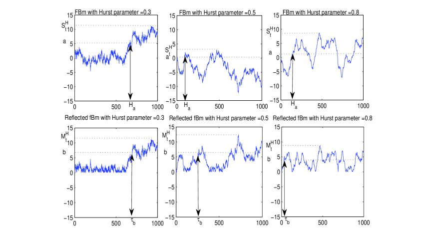
Figure 1: Fractional Brownian motion and their reflections around zero with Hurst parameters H=0.3,H=0.5,H=0.8

Theorem 2.1

For fBm with Hurst parameter $H>\frac{1}{2}$ and $a\in\mathbb{R_{+}}$

$$(M^{H}_{a})^{2}\stackrel{{\scriptstyle law}}{{=}}(\frac{a}{\tau_{1}})^{2H}~{}~{}and~{}~{}(S^{H}_{a})^{2}\stackrel{{\scriptstyle law}}{{=}}(\frac{a}{H_{1}})^{2H}$$

The second moment

$$E(M^{H}_{a})^{2}\leq a^{2H}$$

Proof.

For $x>0,$ by equation (8) we obtain

$$P((\frac{a}{\tau_{1}})^{2H}\leq x) = P(\tau_{1}\geq\frac{a}{x^{1/2H}})=P(\sup_{0\leq t\leq\frac{a}{x^{1/2H}}}|B^{H}_{t}|\leq 1)$$

$$= P(\sup_{0\leq u\leq a}|B^{H}_{\frac{u}{x^{1/2H}}}|\leq 1)=P(\sup_{0\leq u\leq a}|B^{H}_{u}|\leq\sqrt{x})=P((M^{H}_{a})^{2}\leq x)$$

Hence, it is seen that

$$(M^{H}_{a})^{2}\stackrel{{\scriptstyle law}}{{=}}(\frac{a}{\tau_{1}})^{2H}.$$

Now note that,

$$P(\sup_{0\leq u\leq a}|B^{H}_{u}|\leq\sqrt{x}) = P(\sup_{0\leq u\leq a}B^{H}_{u}\leq\sqrt{x},\inf_{0\leq u\leq a}B^{H}_{u}\geq\sqrt{x})$$

$$\leq P(\sup_{0\leq u\leq a}B^{H}_{u}\leq\sqrt{x})=P((S^{H}_{a})^{2}\leq x)$$

And by following the same argument given in (2) it is also observed that

$$(S^{H}_{a})^{2}\stackrel{{\scriptstyle law}}{{=}}(\frac{a}{H_{1}})^{2H}.$$

Hence, combining the equations (2) and (2) the following inequality can be obtained

$$P((M^{H}_{a})^{2}\leq x)\leq P((S^{H}_{a})^{2}\leq x)=P((\frac{a}{H_{1}})^{2H}\leq x)$$

Now, by applying the properties of the Gamma distribution, for $x>0,$ $k>0$ and $\theta>0$ we have

$$\int^{\infty}_{0}\frac{x^{k-1}e^{-\frac{x}{\theta}}}{\Gamma(k)}dx=\theta^{k}.$$ (15)

Therefore

$$E((M^{H}_{a})^{2})\leq E((S^{H}_{a})^{2})=a^{2H}E((\frac{1}{H_{1}})^{2H})=a^{2H}\int^{\infty}_{0}E(e^{-xH_{1}^{2H}})dx$$

For a standard Brownian motion $W,$ it is well known that $E(e^{-\lambda T_{a}})=e^{-a\sqrt{2\lambda}},$ where $T_{a}$ denotes the first hitting time of level $a$ for standard Brownian motion. It was shown in [7] that, for fBm with Hurst parameter $H>\frac{1}{2}$ the following inequality holds

$$E(e^{-\lambda H^{2H}_{a}})\leq e^{-a\sqrt{2\lambda}}$$ (16)

for all $\lambda,a>0.$

Therefore, by equation (16)

$$a^{2H}\int^{\infty}_{0}E(e^{-x\tau_{1}^{2H}})dx\leq a^{2H}\int^{\infty}_{0}e^{-\sqrt{2x}}dx=a^{2H}$$ (17)

As a result, $E((M^{H}_{a})^{2})\leq a^{2H}.$ $\square$

Corollary 2.1

For fBm with Hurst parameter $H>\frac{1}{2}$ and $a\in\mathbb{R_{+}}$

$$P(M^{H}_{a}>x)\leq P(S^{H}_{a}>x)\leq\frac{a^{H}}{x}$$

Proof.

Note that, by Jensen’s inequality

$$E^{2}(S^{H}_{a})\leq E((S^{H}_{a})^{2})\leq a^{2H}$$

As a consequence, $E(M^{H}_{a})\leq E(S^{H}_{a})\leq a^{H}.$

Now, by Markov’s inequality, it is seen that

$$P(M^{H}_{a}>x)\leq P(S^{H}_{a}>x)\leq\frac{a^{H}}{x}$$

$\square$

The bounds given above already are very useful information for the investors because it tells the investor the probability of the values of the supremum up to a fixed time.

In the next theorem a closer upper bound is obtained for the distribution of the supremum of fBm which actually provides better information for the investors.

Theorem 2.2

Consider fBm up to time $a,$ with Hurst parameter $H>\frac{1}{2},$

$$P(S^{H}_{a}\geq x)\leq\frac{\sqrt{2}a^{H}}{x\sqrt{\pi}}$$

Proof.

Now, consider taking fBm up to time $T,$ where $T$ is exponentially distributed random variable with mean $1/\lambda,$ independent of underlying fBm, $B.$ Then using self similarity property of fBm,

$$P(H^{2H}_{a}\leq T)=P(S_{T^{\frac{1}{2H}}}\geq a)=E(e^{-\lambda H^{2H}_{a}})\leq e^{-a\sqrt{2\lambda}}$$ (18)

and hence

$$E(S_{T^{\frac{1}{2H}}})=\int_{0}^{\infty}P(S_{T^{\frac{1}{2H}}}\geq a)\leq\frac{1}{\sqrt{2\lambda}}$$ (19)

Again by the self similarity property we have,

$$E(\sup_{0\leq u\leq T^{\frac{1}{2H}}}B_{u})=E(T^{1/2}\sup_{0\leq u\leq 1}B_{s})=E(\sqrt{T})E(S_{1})$$ (20)

where $E(T^{p/2})=\frac{\Gamma(\frac{2+p}{2})}{\lambda^{p/2}}.$

One can see [8], for details related to taking a random process up to a random time which is independent of the underlying process.

Therefore we obtain

$$E(S_{1})\leq\frac{\sqrt{2}}{\sqrt{\pi}}$$

And by the Markov’s Inequality for any $x>0,$ we can write

$$P(S_{1}\geq x)\leq\frac{E(S_{1})}{x}=\frac{\sqrt{2}}{x\sqrt{\pi}}.$$ (21)

Now by using the scaling property, for any fixed time $a$ we observe

$$P(\sup_{0\leq u\leq a}B^{H}_{u}\leq x) = P(a^{H}\sup_{0\leq u\leq 1}B^{H}_{u}\leq x)=P(a^{H}S^{H}_{1}\leq x)$$

$$= P(S^{H}_{1}\leq\frac{x}{a^{H}})$$

$\square$

3 Application of the results to financial mathematics

In finance, depending on the investor’s demand, risk can be defined in many ways. One of the commonly used definitions of risk is known as $"downfalls"$ or $"maximum~{}~{}drawdown".$ Maximum drawdown is the highest possible loss in the price of one share of the risky asset. One of the fundamental results related to a standard Brownian motion is L$\acute{e}$vy Theorem (see [4]). This theorem leads us to the result that $"maximum~{}~{}drawdown",$ the highest possible loss in the trajectories of the standard Brownian motion is identical in law with the supremum of the reflected Brownian motion. In other words, the $"maximum~{}~{}drawdown",$ before time $t$ is defined as

$$D^{-}_{t}:=\sup_{0\leq u\leq v\leq t}(W_{u}-W_{v})=\sup_{0\leq v\leq t}(\sup_{0\leq u\leq v}W_{u}-W_{v})$$

and it satisfies

$$(\sup_{0\leq u\leq v}W_{u}-W_{v})\stackrel{{\scriptstyle law}}{{=}}(\sup_{0\leq v\leq t}|W_{v}|)$$

by the L$\acute{e}$vy isomorphism.

In the above result, we would like to replace standard Brownian motion with fBm, because it is obvious that fBm is a more realistic model than a standard Brownian motion for the risky assets. In the literature, due to the complex nature of fBm there are not many exact results on the distributions related to the trajectories. For this reason, we also expect to obtain not exact results but some bounds.

In the fBm notation let,

$$D^{-,H}_{t}:=\sup_{0\leq a^{\prime}\leq a\leq t}(B_{a^{\prime}}-B_{a})=\sup_{0\leq a\leq t}(\sup_{0\leq a^{\prime}\leq a}B_{a^{\prime}}-B_{a})$$

be the $"maximum~{}~{}drawdown".$

Our goal is to find the exact distribution or alternatively find bounds for the distribution of $"maximum~{}~{}drawdown",$ which is directly applicable to finance, however we have not been able to obtain that, yet. In this study, we would like to present a lower bound for the distribution of the difference between the supremum of fBm and the value of fBm at time $a,$ which is the first step of finding a lower bound for the distribution of $"maximum~{}~{}drawdown"$ of fBm up to time $t.$ And this following result will be extended to finding the distribution of $"maximum~{}~{}drawdown"$ in the later studies.

Now, let

$$Y^{H}_{a}:=S^{H}_{a}-B^{H}_{a}$$ (23)

be the difference between the supremum of fBm up to time $a$ and the value of fBm at time $a.$

Theorem 3.1

For $y\geq 0,$

$$P(Y^{H}_{a}\leq y)\geq 1-\frac{\sqrt{2}a^{H}}{y\sqrt{\pi}}$$

Proof.

For $a\in\mathbb{R_{+}},$

$$P(S^{H}_{a}\geq b) = P(S^{H}_{a}\geq b,B^{H}_{a}\geq b)+P(S^{H}_{a}\geq b,B^{H}_{a}<b)$$ (24)

$$= P(B^{H}_{a}\geq b)+P(S^{H}_{a}\geq b,B^{H}_{a}<b)\leq\frac{\sqrt{2}a^{H}}{x\sqrt{\pi}}$$

by Theorem (2.2).

Thus we have,

$$0\leq P(S^{H}_{a}\geq b,B^{H}_{a}<b)\leq\frac{\sqrt{2}a^{H}}{b\sqrt{\pi}}-P(B^{H}_{a}\geq b)$$ (25)

For $b\geq x,$ $x\in\mathbb{R_{+}},$

$$P(B^{H}_{a}<x)-P(S^{H}_{a}<b,B^{H}_{a}<x)$$ (26)

$$= P(S^{H}_{a}\geq x,B^{H}_{a}<x)\leq P(S^{H}_{a}\geq b,B^{H}_{a}<b)\leq\frac{\sqrt{2}a^{H}}{b\sqrt{\pi}}-P(B^{H}_{a}\geq b)$$

by (25) and since $x\leq b.$ Therefore, we have

$$P(S^{H}_{a}<b,B^{H}_{a}<x)\geq P(B^{H}_{a}<x)+P(B^{H}_{a}\geq b)-\frac{\sqrt{2}a^{H}}{b\sqrt{\pi}}$$ (27)

Now as a result, we get

$$P(Y^{H}_{a}\leq y,B^{H}_{a}\leq x)\geq P(B^{H}_{a}<x)+P(B^{H}_{a}\geq y+x)-\frac{\sqrt{2}a^{H}}{(y+x)\sqrt{\pi}}$$ (28)

by (23), where $y=b-x$ and

$$P(Y^{H}_{a}\leq y,B^{H}_{a}\in dx)\geq P(B^{H}_{a}\in dx)+\frac{dP(B^{H}_{a}\geq y+x)}{dx}-\frac{\sqrt{2}a^{H}}{(y+x)^{2}\sqrt{\pi}}$$

finally

$$P(Y^{H}_{a}\geq y)\geq\int^{\infty}_{0}P(B^{H}_{a}\in dx)+\int^{\infty}_{0}\frac{dP(B^{H}_{a}\geq y+x)}{dx}dx-\int^{\infty}_{0}\frac{\sqrt{2}a^{H}}{(y+x)^{2}\sqrt{\pi}}dx$$

Hence, for $y\geq 0,$

$$P(Y^{H}_{a}\leq y) \geq \frac{1}{2}+\int^{\infty}_{0}dP(B^{H}_{a}\geq y+x)-\int^{\infty}_{0}\frac{\sqrt{2}}{(y+x)^{2}\sqrt{\pi}}dx$$ (29)

$$= \frac{1}{2}-\frac{\sqrt{2}a^{H}}{\sqrt{\pi}y}+\int^{\infty}_{0}dP(B^{H}_{a}\geq y+x)$$

And by the Fundamental Theorem of Calculus,

$$P(Y^{H}_{a}\leq y)\geq\frac{1}{2}-\frac{\sqrt{2}a^{H}}{\sqrt{\pi}y}+\int^{\infty}_{0}\frac{1}{\sqrt{2\pi}}e^{\frac{-(x+y)^{2}}{2}}dx=1-\frac{\sqrt{2}a^{H}}{\sqrt{\pi}y}$$ (30)

$\square$

4 Conclusion

The Black-Scholes model for the values of the log returns of a risky stock using fBm is a more realistic model than using standard Brownian motion, due the advantage of its capability of displaying the dependence of increments. The investors of the risky stocks or their derivatives, would naturally be interested in the highest value of the asset, in a certain time period. Towards that end, we have provided an upper bound on the second moment of the supremum of reflected fBm as a first result, and based on this, we have given an upper bound on the distribution of the supremum of reflected fBm.

Later, we have observed a lower bound on the distribution of the supremum of fBm up to time $1$ as well as up to fixed time $a.$ As an application of the second result, we have given the joint distribution of the supremum of fBm up to time $a$ and the value of fBm at time $a$ and obtained a lower bound on the distribution of the difference between them. Obviously, this application is already very useful for the investors. Based on the given results, we will investigate the distribution of ”maximum drawdown” because of its important use as a measure of risk, in finance, as future work. Our conjecture on this distribution is, that it is both related to the distribution of the supremum of the reflected fBm and the distribution of the difference between the supremum of fBm and the value of fBm at the maturity time.

5 Acknowledgement

Ceren Vardar would like to thank Mine Caglar from Koc University, Istanbul for her warm and generous support for this study. She would also like to thank Craig L. Zirbel from Bowling Green State University, Ohio and Gabor J. Szekely from National Science Foundation, Washington D.C for introducing her to the subject.

References

- [1] Biagini, F., Hu, Yaozhong., Oksendal, B., Zhang Tusheng. Stochastic Calculus for Fractional Brownian Motion and Applications. Springer Verlag, London, 2008.
- [2] Kolmogorov, A.N. Wienersche Spiralen und einige andere interessante Kurven im Hilbertschen Raum. C.R.(Doklady) Acad. URSS(N.S) 26, 115-118, (1940).
- [3] Mandelbrot, B.B. and Van Ness, J.W. Fractional Brownian motions, fractional noises and applications. SIAM Rev. 10, 422-437, 1968.
- [4] Revuz, D., Yor, R. Continuous Martingales and Brownian Motion. Springer Verlag, Berlin, Hiedelberg, 2001.
- [5] Rogers, L. C. G. Arbitrage with fractional Brownian motion. Mathematical Finance, 7 (1997) 95-105.
- [6] Douady, A.N., Shiryaev, Yor, M. On probability charateristics of ”downfalls” in a standard Brownian motion. Theory Prob. Appl., 44 (1999) 29-38.
- [7] Decreusefond, L. and Nualart, D. Hitting Times For Gaussian Processes. The Annals of Prob., 36 (2008) 319-330.
- [8] Salminen, P., Vallois, P. On maximum increase and decrease of Brownian Motion. Annales de l’institut Henri Poincare (B) Probabilit s et Statistiques, 43 no. 6 (2007) 655-676
- [9] Bertoin, J. Levy Processes. Cambridge University Press, Cambridge, UK, 1996.
- [10] Lvy, P. Processus Stochatiques et Mouvement Brownien, Gauthier-Villars, Paris, 1948.
- [11] Abry, P. and Sellan, F. The Wavelet-Based Synthesis for Fractional Brownian Motion Proposed by F. Sellan and Y. Meyer: Remarks and Fast Implementation. Appl. Comp. Harmonic Anal. 3 (1996) 337-383
- [12] Sellan, F. Synthse de Mouvements Browniens Fractionaires l’aide de la Transformation par Ondelettes. C.R. Acad. Sci. Paris Ser. Math., 321 (1995) 351-358
- [13] Caglar, M. Simulation of Fractional Brownian Motion with Micropulses. Advances in Performance Analysis, 3 no. 1 (2000) 43-69