Transient behavior of heat transport in a thermal switch

Abstract

We study the time-dependent transport of heat in a nanoscale thermal switch. The switch consists of left and right leads that are initially uncoupled. During switch-on the coupling between the leads is abruptly turned on. We use the nonequilibrium Green’s function formalism and numerically solve the constructed Dyson equation to determine the nonperturbative heat current. At the transient regime we find that the current initially flows simultaneously into both of the leads and then afterwards oscillates between flowing into and out of the leads. At later times the oscillations decay away and the current settles into flowing from the hotter to the colder lead. We find the transient behavior to be influenced by the extra energy added during switch-on. Such a transient behavior also exists even when there is no temperature difference between the leads. The current at the long-time limit approaches the steady-state value independently calculated from the Landauer formula.

The physics of generation, dissipation, and manipulation of heat in nanoscale systems is an important topic that has recently gathered attention. Experiments on molecular junctions moljuncexp found that the heat generated in current-carrying metal-molecule junctions is substantial and can affect the integrity of the device. Understanding how to efficiently dissipate extraneous heat in nanoscale systems is thus imperative in the construction of devices. In addition, the movement of heat may be harnessed for information processing infoproc . Recent experiments have shown the viability of thermal transistors saira07 , thermal rectifiers using inhomogeneous carbon and boron nitride nanotubes chang06 , and conductance-tunable thermal links consisting of multiwalled carbon nanotubes chang07 .

Most of the above-mentioned work, however, focus on the examination of steady-state phenomena. In contrast, any physical device must function in a time-dependent environment. Although some work has been done in the study of time-dependent electronic transport electronic , the investigation of time-dependent behavior in quantum heat transport has not yet attracted much attention velizhanin08 . Developing theoretical tools and computational methods for such problems are thus essential to the progress of the field. In this paper we study the time-dependent heat current in a junction system we call a thermal switch. We generalize the nonequilibrium Green’s function formalism wang08 , which is developed for steady-state situations, to the time-dependent case with a well-defined initial thermal state. To get nonperturbative results, the key steps we take are to construct and numerically solve a Dyson equation that does not satisfy time-translational invariance.

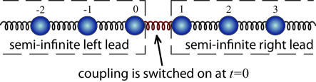
Figure 1: (color online) An illustration of a quantum thermal switch. The labels of the first $3$ sites in each lead are shown. The coupling between sites $0$ and $1$ is switched on at $t=0$.

Fig. 1 shows a one-dimensional chain having a coupling that can be switched on and off. The semi-infinite left and right leads are linear chains of masses $m$. Each atom interacts with its left and right neighbors through an interparticle harmonic potential having spring constant $k$. An on-site harmonic potential, with spring constant $k_{0}$, is also experienced by each atom. During time $t<0$ the left and right leads are uncoupled and are in thermal equilibrium with temperatures $T_{\rm L}$ and $T_{\rm R}$, respectively. At time $t=0$ the coupling potential, in the form of an interparticle harmonic potential with the same spring constant $k$, is switched on, i.e., the potential between the masses labeled $0$ and $1$ in Fig. 1 is suddenly switched on. We then want to know how the time-dependent heat current behaves in such a setup. In experiments on molecular junctions moljuncexp a scanning tunneling microscope tip is used to stretch a molecule until a bond in the molecule breaks. In the thermal switch we can think of the switch-on as the inverse process, i.e., a bond is induced through proximity.

The leads follow the Hamiltonian

$$H^{\alpha}=\frac{1}{2}\sum_{i}\dot{u}_{i}^{\alpha}\dot{u}_{i}^{\alpha}+\frac{1}{2}\sum_{ij}u_{i}^{\alpha}K_{ij}^{\alpha}u_{j}^{\alpha},~{}~{}~{}\alpha={\rm L,R},$$ (1)

where the sums are over all sites in the lead, the transformed coordinates are given by $u_{i}=\sqrt{m}\,x_{i}$, $x_{i}$ is the relative displacement of the $i$-th atom of mass $m$, and $K^{\alpha}$ is the spring constant matrix. The $K^{\rm L}$ and $K^{\rm R}$ matrices are semi-infinite tridiagonal matrices with $2k+k_{0}$ along the diagonal and $-k$ along the off-diagonal. The Hamiltonian for the switched coupling is

$$H^{\rm LR}=\sum_{ij}u^{\rm L}_{i}V^{\rm LR}_{ij}u^{\rm R}_{j}.$$ (2)

The coupling constant matrices $V^{\rm LR}$ and $V^{\rm RL}$ are zero matrices during $t<0$. After the switch-on, $V^{\rm LR}$ has one non-zero element $V^{\rm LR}_{01}=-k$ and $V^{\rm RL}$ has the lone non-zero element $V^{\rm RL}_{10}=-k$, where the matrix indices correspond to the labels of the masses in the leads. Note that $H^{\rm LR}=H^{\rm RL}$. The time-dependent governing Hamiltonian therefore is $H(t)=H^{\rm L}+H^{\rm R}+H^{\rm LR}~{}\theta\left(t\right)$, where $\theta\left(t\right)$ is the Heaviside step function.

The current flowing out of the left lead $I_{\rm L}(t)=-\left<dH^{\rm L}/dt\right>$, i.e., it is the expectation value of the rate of change in $H^{\rm L}$. When the switch is turned on the current is given by

$$I_{\rm L}\left(t\right)=\hbar k~{}{\rm Im}\!\left[\frac{\partial G^{\rm RL,<}\left(t_{1},t_{2}\right)}{\partial t_{2}}\right]_{t_{1}=t_{2}=t},$$ (3)

where “${\rm Im}$” stands for the imaginary part. The lesser Green’s function that appears in the formula is defined as $G^{\rm RL,<}\left(t_{1},t_{2}\right)=-\frac{i}{\hbar}\bigl{\langle}u^{\rm L}_{0}\left(t_{2}\right)u^{\rm R}_{1}\left(t_{1}\right)\bigr{\rangle}$, where the subscripts $0$ and $1$ correspond to the labels of the masses. Note that this is a two-time correlation function that does not satisfy time-translational invariance, i.e., its time-dependence can not be written as a difference $t_{1}-t_{2}$. Similarly, the current flowing out of the right lead, $I_{\rm R}(t)=-\left<dH^{\rm R}/dt\right>$, when the switch is turned on is in the form of Eq. (3) except that the ${\rm R}$ and ${\rm L}$ superscripts are swapped.

To determine the full, nonperturbative, current we are going to solve the associated Dyson equation. First, we define the contour-ordered Green’s function haug96

$$G^{\rm RL}\left(\tau_{1},\tau_{2}\right)=-\frac{i}{\hbar}\left<{\rm T}_{c}u^{\rm R}_{1}\left(\tau_{1}\right)u^{\rm L}_{0}\left(\tau_{2}\right)\right>,$$ (4)

where the $u^{\rm R}_{1}$ and $u^{\rm L}_{0}$ are Heisenberg operators, ${\rm T}_{c}$ is the contour-ordering operator, and $\tau_{1}$ and $\tau_{2}$ are complex variables on the contour $C$. To determine the current at time $t$ we employ a Keldysh contour $C$ that goes from time $0$ to $t$ and then back to $0$. Since the left and right leads are uncorrelated before the switch is turned on at time $0$, the contour does not have a complex tail after it goes back to time $0$.

Converting to the interaction picture the contour-ordered Green’s function shown in Eq. (4) becomes

$$G^{\rm RL}\left(\tau_{1},\tau_{2}\right)\!=\!-\frac{i}{\hbar}\!\left<\!{\rm T}_{c}e^{-\frac{i}{\hbar}\int_{C}d\tau^{\prime}H^{\rm LR}(\tau^{\prime})}u^{\rm R}_{1}\left(\tau_{1}\right)u^{\rm L}_{0}\left(\tau_{2}\right)\right>.$$ (5)

A perturbative calculation can then be done by expanding the exponential as an infinite series. We can also use this expansion in constructing the Dyson equation. In the series, the zeroth-order term vanishes because it does not contain the coupling potential. Furthermore, all the even-ordered terms also vanish because there will be an extra $u^{\rm R}$-$u^{\rm L}$ pair without a connecting coupling potential. Thus, only the odd-ordered terms survive.

We can use diagrams in constructing the Dyson equation. Shown in Fig. 2 is the resulting diagram equation when we expand the series in Eq. (5). A double-line diagram represents $G^{\rm RL}$, a single line represents the equilibrium Green’s functions for the right lead, $g^{\rm R}\left(\tau_{1},\tau_{2}\right)=-\frac{i}{\hbar}\left<{\rm T}_{c}u^{\rm R}_{1}\left(\tau_{1}\right)u^{\rm R}_{1}\left(\tau_{2}\right)\right>_{0}$, and a dashed line represents the equilibrium Green’s functions for the left lead, $g^{\rm L}\left(\tau_{1},\tau_{2}\right)=-\frac{i}{\hbar}\left<{\rm T}_{c}u^{\rm L}_{0}\left(\tau_{1}\right)u^{\rm L}_{0}\left(\tau_{2}\right)\right>_{0}$. The subscript $0$ implies that the average is taken with respect to equilibrium distributions that are maintained when $t<0$ before the switch-on.

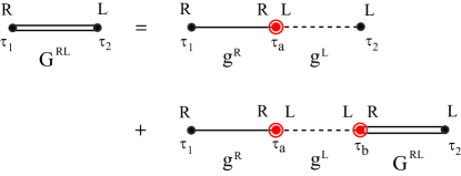
Figure 2: (color online) Diagram representation of the Dyson equation. Each line is labelled by the Green’s function it represents. Each concentric dot represents a coupling vertex.

Rewriting the diagram equation in Fig. 2 as contour integrals, we have

$$G^{\rm RL}\left(\tau_{1},\tau_{2}\right) = \int_{C}d\tau_{a}~{}g^{\rm R}\left(\tau_{1},\tau_{a}\right)V^{\rm RL}~{}g^{\rm L}\left(\tau_{a},\tau_{2}\right)$$ (6)

$$+~{}\int_{C}d\tau_{a}\int_{C}d\tau_{b}~{}g^{\rm R}\left(\tau_{1},\tau_{a}\right)V^{\rm RL}$$

$$\times~{}g^{\rm L}\left(\tau_{a},\tau_{b}\right)V^{\rm LR}~{}G^{\rm RL}\left(\tau_{b},\tau_{2}\right).$$

Applying Langreth’s theorem to Eq. (6) and then iterating haug96 , we should obtain an expression for $G^{\rm RL,<}$. To calculate the current in Eq. (3) we need the time derivative of $G^{\rm RL,<}$, and so we differentiate it to get

$$\frac{\partial G^{\rm RL,<}\left(t_{1},t_{2}\right)}{\partial t_{2}} = \frac{\partial G^{\rm RL,<}_{1}\left(t_{1},t_{2}\right)}{\partial t_{2}}$$ (7)

$$- k\int^{t}_{0}dt_{a}~{}G^{\rm RL,r}\left(t_{1},t_{a}\right)\frac{\partial G^{\rm RL,<}_{1}\left(t_{a},t_{2}\right)}{\partial t_{2}}$$

$$- k\int^{t}_{0}dt_{a}~{}G^{\rm RL,<}_{1}\left(t_{1},t_{a}\right)\frac{\partial G^{\rm RL,a}\left(t_{a},t_{2}\right)}{\partial t_{2}}$$

$$+ k^{2}\int^{t}_{0}dt_{a}\int^{t}_{0}dt_{b}~{}G^{\rm RL,r}\left(t_{1},t_{a}\right)$$

$$\times G^{\rm RL,<}_{1}\left(t_{a},t_{b}\right)\frac{\partial G^{\rm RL,a}\left(t_{b},t_{2}\right)}{\partial t_{2}},$$

where

$$G^{\rm RL,<}_{1}\left(t_{1},t_{2}\right) = -k\int^{t}_{0}dt_{a}\left\{g^{\rm R,r}\left(t_{1}-t_{a}\right)~{}g^{\rm L,<}\left(t_{a}-t_{2}\right)\right.$$ (8)

$$+~{}\left.g^{\rm R,<}\left(t_{1}-t_{a}\right)~{}g^{\rm L,a}\left(t_{a}-t_{2}\right)\right\}$$

is the first-order term in the perturbation series in Eq. (5). The analytic expressions for the equilibrium surface Green’s functions $g^{\rm R,r}$, $g^{\rm R,<}$, $g^{\rm L,<}$, and $g^{\rm L,a}$ are known in frequency space wang07 . To determine their time-dependence we numerically calculate their corresponding Fourier transforms.

The other unknowns in Eq. (7) involve the retarded and advanced versions of the full Green’s function. We can apply Langreth’s theorem again to Eq. (6) to determine expressions for these unknowns. We get

$$G^{\rm RL,\beta}\left(t_{1},t_{2}\right) = -k\int^{t}_{0}dt_{a}~{}G^{\rm RL,\beta}_{1}\left(t_{1},t_{a}\right)G^{\rm RL,\beta}\left(t_{a},t_{2}\right)$$ (9)

$$+~{}G^{\rm RL,\beta}_{1}\left(t_{1},t_{2}\right),$$

where $\beta={\rm r,a}$, and the first-order term is

$$G^{\rm RL,\beta}_{1}\left(t_{1},t_{2}\right)=-k\int^{t}_{0}dt_{a}~{}g^{\rm R,\beta}\left(t_{1}-t_{a}\right)~{}g^{\rm L,\beta}\left(t_{a}-t_{2}\right).$$ (10)

To solve Eq. (9) we discretize the time variable into $N$ segments and thus transforming the integral into a sum. This results in a linear problem of the form ${\bf A}\vec{x}=\vec{b}$, where the unknown $\vec{x}$ is determined by performing an LU decomposition on ${\bf A}$ and then using $\vec{b}$ in the back-substitution. The $\partial G^{\rm RL,a}\left(t_{a},t_{2}\right)/\partial t_{2}$ term required in Eq. (7) can also be calculated by first differentiating Eq. (9) and then finding the solution to the resulting equation with the time discretized. By determining the time derivative of the full Green’s function in Eq. (7) the current that we calculate is a nonperturbative result. We follow the same steps to independently calculate the current flowing out of the right lead.

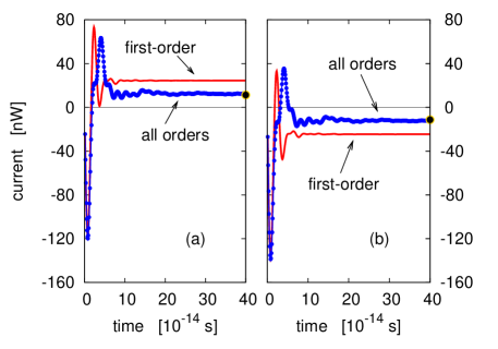
Figure 3: The time-dependent current flowing out of the (a) left lead and (b) right lead. The (blue online) data points are results from solving the Dyson equation while the (red online) line is the result from the first-order perturbation calculation. The average temperature between the leads is $T=300~{}{\rm K}$. The interparticle spring constant is $k=0.625$ eV/(Ų u) while the on-site spring constant is $k_{0}=0.0625$ eV/(Ų u).

Shown in Fig. 3 are plots of the time-dependent current flowing out of the leads when the left and right lead temperatures are $T_{\rm L}=330$ K and $T_{\rm R}=270$ K, respectively. The average temperature is thus $T=300$ K with offsets of $\pm 10\%$. The currents oscillate at a frequency comparable to the highest phonon frequencies available in the system and then gradually decay to their steady-state values. The dots shown at the right edges of the plots are steady-state values calculated independently from the Landauer formula $I_{\rm L}=-I_{\rm R}=\frac{1}{2}\int^{\infty}_{-\infty}\frac{d\omega}{2\pi}~{}\hbar\omega\left(f_{\rm L}-f_{\rm R}\right)\tilde{\theta}\left(\omega\right)$, where $f_{\rm L}$ and $f_{\rm R}$ are the Bose-Einstein distributions of the left and right leads, respectively, and $\tilde{\theta}\left(\omega\right)$ is $1$ within the phonon band, $k_{0}<\omega^{2}<4k+k_{0}$, and $0$ otherwise wang07 . At steady-state, heat should flow from the hotter to the colder lead, i.e., from the left to the right lead. Thus, the sign of the current flowing out of the left lead should be positive and for the right lead negative. However, during the transient time, the current can flow in unexpected directions. Just after the switch-on, the current actually does not flow from the hotter to the colder lead. In Fig. 3 we see the current to flow simultaneously into both of the leads. There appears to be an energy source in-between the leads that supply the current. Recall that there is no coupling between the leads before the switch-on. By turning on the switch we actually add energy, in the form of the switched coupling potential, to the system. This added coupling energy supplies the current that flows into both leads. In Fig. 3 we also compare the results from first-order perturbation to the results from nonperturbative calculations. Unlike the perturbative results, nonperturbative results approach the steady-state values at later times. Since the switched coupling has the same strength as the interparticle potential we indeed expect corrections to perturbative calculations to be significant.

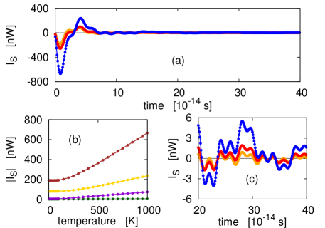
Figure 4: (a) Plots of $I_{\rm S}=I_{\rm L}+I_{\rm R}$ as functions of time when $T=10$ K (orange online), $T=300$ K (red online), and $T=1000$ K (blue online). The temperature offsets are $\pm 10\%$. (b) Plots of $\left|I_{\rm S}\right|$ as functions of $T$ at time $t=0.8~{}[t]$ (brown online), $t=4.1~{}[t]$ (yellow online), $t=6.0~{}[t]$ (violet online), and $t=23.0~{}[t]$ (green online), where $[t]=10^{-14}$ s. (c) An enlarged view of (a) for time $t=20~{}[t]$ to $t=40~{}[t]$.

Shown in Fig. 4 are plots of the sum of the currents, $I_{\rm S}=I_{\rm L}+I_{\rm R}$, as functions of the time and the average temperature of the leads. $I_{\rm S}$ fluctuates around zero with a fluctuation amplitude that decays with time. Fig. 4(b) shows $I_{\rm S}$ to vary strongly with temperature at the transient regime. As time goes on $I_{\rm S}$ slowly loses its dependence on temperature. Fig. 4(c) shows that at later times fluctuations in $I_{\rm S}$ still appear but are significantly smaller than those at the transient regime. We do expect that at the steady state, of which the long-time limit of our data approaches, all of the current flowing out of the left lead should flow into the right lead and thus resulting in $I_{\rm S}=0$, regardless of the value of the temperature. However, since energy is added during the switch-on, this extra energy influences the transient behavior of the system until it eventually dissipates out to the heat baths. Fitting the envelope to an exponential function we find a characteristic decay time of about $10\times 10^{-14}$ s. At any particular time $t$ we can determine the energy the system absorbs or emits from $\left<H^{\rm LR}\left(t\right)\right>=\int_{0}^{t}\left(I_{\rm L}+I_{\rm R}\right)dt$.

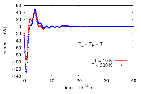
Figure 5: The current flowing through the junction when the left and right leads have the same temperature. $T=10$ K (red online) and $T=300$ K (blue online).

Suppose we set the temperatures of the leads to be the same. Shown in Fig. 5 is the time-dependent current, in either lead since the leads are indistinguishable, for such a situation. At the steady state there should be no current flowing within the system. However, since energy is added to the system during the switch-on, at the transient regime we see a fluctuating current with temperature-dependent amplitude flowing within the system.

The method can also be generalized in a straightforward manner to deal with a time-varying coupling that is on during $t>0$. For a mildly increasing coupling such as, for example, $k(t)=k\tanh(ft)$, the transient current also initially flows simultaneously into both of the leads. This transient behavior persists because switching on the coupling introduces energy, that has to dissipate into the baths, into the system.

To summarize, we have shown an exact nonperturbative method to calculate the time-dependent heat current in a thermal switch using nonequilibrium Green’s functions. The Dyson equation is constructed using Keldysh contours and the real-time Green’s functions needed to calculate the current are determined by applying Langreth’s theorem to the Dyson equation and numerically solving the equation with the discretized time variable. We set the strength of the switched coupling to be the same as the interparticle spring constant. Nonperturbative results are thus significantly different from perturbative ones. We find the transient current just after the switch-on to be influenced by the extra switched coupling energy. In particular, the initial reaction after switch-on is for the current to flow simultaneously into both the left and right leads. The current then oscillates with amplitude that decays with time. In the long-time limit the current approaches the expected steady-state values calculated independently from the Landauer formula. We also note that the theory presented here is not restricted only to one-dimensional chains but is applicable to any junction system where a thermal switch-on occurs.

We are grateful to Lifa Zhang, Jin-Wu Jiang, Meng Lee Leek, and Jose Garcia for insightful discussions. This work is supported in part by an NUS research grant number R-144-000-257-112.

References

- (1) Z. Huang, B. Xu, Y. Chen, M. Di Ventra, and N. Tao, Nano Lett. 6, 1240 (2006); Z. Huang, F. Chen, R. D’Agosta, P.A. Bennett, M. Di Ventra, and N. Tao, Nature Nanotech. 2, 698 (2007); M. Tsutsui, M. Taniguchi, and T. Kawai, Nano Lett. 8, 3293 (2008).
- (2) M. Terraneo, M. Peyrard, G. Casati, Phys. Rev. Lett. 88, 094302 (2002); B. Li, L. Wang, and G. Casati, Phys. Rev. Lett. 93, 184301 (2004); D. Segal and A. Nitzan, Phys. Rev. Lett. 94, 034301 (2005); L. Wang and B. Li, Phys. Rev. Lett. 99, 177208 (2007).
- (3) O.-P. Saira, M. Meschke, F. Giazotto, A.M. Savin, M. Möttönen, and J.P. Pekola, Phys. Rev. Lett. 99, 027203 (2007).
- (4) C.W. Chang, D. Okawa, A. Majumdar, and A. Zettl, Science 314, 1121 (2006).
- (5) C.W. Chang, D. Okawa, H. Garcia, T.D. Yuzvinsky, A. Majumdar, and A. Zettl, Appl. Phys. Lett. 90, 193114 (2007).
- (6) G. Stefanucci and C.-O. Almbladh, Phys. Rev. B 69, 195318 (2004); J. Maciejko, J. Wang, and H. Guo, Phys. Rev. B 74, 085324 (2006); V. Moldoveanu, V. Gudmundsson, and A. Manolescu, Phys. Rev. B 76, 085330 (2007); Z. Feng, J. Maciejko, J. Wang, and H. Guo, Phys. Rev. B 77, 075302 (2008).
- (7) K.A. Velizhanin, H. Wang, and M. Thoss, Chem. Phys. Lett. 460, 325 (2008).
- (8) See, for a review, J.-S. Wang, J. Wang, and J.T. Lü, Eur. Phys. J. B 62, 381 (2008).
- (9) See, for example, H. Haug and A.-P. Jauho, Quantum Kinetics in Transport and Optics of Semiconductors, 2nd ed. (Springer, 2008).
- (10) J.-S. Wang, N. Zeng, J. Wang, and C.K. Gan, Phys. Rev. E 75, 061128 (2007).