Demagnified GWs from Cosmological Double Neutron Stars and GW Foreground Cleaning Around 1Hz

Abstract

Gravitational waves (GWs) from cosmological double neutron star binaries (NS+NS) can be significantly demagnified by strong gravitational lensing effect, and the proposed future missions such as BBO or DECIGO might miss some of the demagnified GW signals below a detection threshold. The undetectable binaries would form a GW foreground which might hamper detection of a very weak primordial GW signal. We discuss the outlook of this potential problem, using a simple model based on the singular-isothermal-sphere lens profile. Fortunately, it is expected that, for presumable merger rate of NS+NSs, the residual foreground would be below the detection limit $\Omega_{GW,lim}\sim 10^{-16}$ realized with BBO/DECIGO by correlation analysis.

I introduction

A GW background from the early universe is one of the primary targets of observational cosmology. It would provide us with crucial information on physics at very high-energy scales. Among others, a primordial GW background generated during an inflationary period is a key objective Allen:1996vm . Currently, there are two approaches to probe the inflation background. One is indirect observation around $f\sim 10^{-18}$Hz through B-mode polarization of cosmic microwave background Seljak:1996gy . Another is direct GW detection around $f\sim 0.1$-1Hz with the proposed space laser interferometers such as the Big Bang Observer (BBO) bbo or the Deci-hertz Interferometer Gravitational Wave Observatory (DECIGO) Seto:2001qf ; Kawamura . These two approaches at widely separated frequencies are complimentary and we might disclose fundamental properties of inflation by using them simultaneously (see e.g. Smith:2005mm ). But, in both of them, we must cope with strong astrophysical contaminations to uncover the inflation background.

At present, the overall profile of astrophysical GW foregrounds around $f\sim 1$Hz is unclear. Although white-dwarf binaries (important for the Laser Interferometer Space Antenna (LISA) lisa ) would not make a critical limit there Farmer:2003pa , we might have a strong foreground component whose quantitative properties are difficult to predict now. This is partly due to the complicated astrophysical processes involved. For example, to estimate the foreground made by supernovae of population III stars, we need, at least, the formation rate of these stars and their angular momentum distribution. But, unfortunately, these important elements are poorly known at present Buonanno:2004tp . Meanwhile, around 1Hz, we also have a foreground made by double neutron star binaries (NS+NSs) that are individually very simple system accurately predicted with the post-Newtonian inspiral waveforms . In addition, NS+NSs are promising target for the first detection of GWs with ground-based detectors, and their coalescence rate has been extensively discussed with the observed abundance of NS+NSs in our galaxy Kalogera:2001dz . Considering our current understanding on the 1Hz band, in this paper, we study only the NS+NS foreground, neglecting other potential but highly uncertain astrophysical foregrounds.

NS+NSs can be regarded as solid GW sources around 1Hz, and cleaning of these binaries would be a critical element for the success of BBO/DECIGO to detect a weak primordial GW background. The basic approach for the cleaning is to identify individual binaries and subtract their chirping waveforms from the data of detectors Cutler:2005qq ; Harms:2008xv . As we see later, in order to fully use the designed sensitivity of detectors for a primordial background, the residual astrophysical foreground after the cleaning must be $\sim 10^{5}$ times smaller than their original strength (in terms of GW energy spectrum).

To discuss the prospect of this cleaning procedure, we first need to understand the detectability of GWs from individual NS+NSs. Since we cannot expect a large fluctuation (e.g. a factor of 2) for the intrinsic chirp mass distribution of NS+NSs, the primary parameter that characterizes the signal-to-noise ratio of a binary would be its distance or equivalently its redshift $z$. Another important parameter of a binary is its inclination angle, which can change the GW amplitude by a factor of $2\sqrt{2}$ (ratio between face-on and edge-on binaries). Therefore, the basic requirement for the cleaning is to make detectors that have enough sensitivities to detect an edge-on NS+NS at high redshift (e.g. $z=10$) Cutler:2005qq .

However, the situation becomes complicated due to the gravitational lensing effect that modulates observed amplitudes of GWs during their propagation between the sources and detectors lens . We might miss some demagnified GW signals which are below a detection threshold, and their resultant residuals might be an obstacle for detecting a weak inflation background. Our principle aim in this paper is to provide a rough outlook on this potential problem caused by gravitational lensing.

Gravitational lensing effects can be broadly divided into two categories: the weak lensing due to accumulated small distortions during wave propagation Bartelmann:1999yn (see also Cutler:2009qv ; Itoh:2009iy for GWs from NS+NSs) and the strong lensing caused by specific massive objects with large distortions lens . We are interested in significantly (e.g. 50%) demagnified lensing fluctuations, but such probability is known to be negligible for weak lensing, even for a high-redshift source Barber:2000pe . Therefore, we concentrate on the strong lensing effect that can generate significant demagnification more frequently. For the lens profile, we use the singular isothermal sphere (SIS) model, which is fairly successful for studying various observational aspects of strong lensing effects lens .

This paper is organized as follows. In Sec. II, we discuss the merger rate of cosmological NS+NSs and their GW foreground. In Sec. III, the strong gravitational lensing effect is studied. The probability distribution function for the faint-end of demagnification is evaluated with the SIS model. Then we estimate the GW foreground made by undetectable NS+NSs. Section IV is devoted to discussions on this paper.

II cosmological NS+NS binaries

In this section, we briefly discuss basic aspects of cosmological NS+NSs and their GWs around 1Hz, following Cutler and Harms Cutler:2005qq . First we evaluate the total merger rate ${\dot{N}}_{T}$ ($T$, total) of cosmological NS+NSs. Based on the observed NS+NSs in our galaxy and the number densities of various types of nearby galaxies, the comoving merger rate at present ${\dot{n}}_{0}$ is estimated to be $10^{-8}$-$10^{-6}{\rm Mpc^{-3}yr^{-1}}$, roughly corresponding to the Advanced-LIGO detection rate $10^{1\pm 1}{\rm yr^{-1}}$ Kalogera:2001dz . To deal with merger events at cosmological distances, we put the comoving merger rate ${\dot{n}}(z)$ at redshift $z$ as follows

$${\dot{n}}(z)=s(z){\dot{n}}_{0}.$$ (1)

Here, the nondimensional function $s(z)$ represents the redshift dependence of the rate, and, in this paper, we consider the following two concrete models: (I) the fiducial evolutionary model $s_{I}(z)$ with a piecewise function

$$s_{I}(z)=\left\{\begin{array}[]{ll}1+2z&(0\leq z\leq 1)\\ 3(5-z)/4&(1<z\leq 5)\\ 0&(5<z),\\ \end{array}\right.$$ (5)

and (II) a simple model

$$s_{II}(z)=\left\{\begin{array}[]{ll}1&(0\leq z\leq 10)\\ 0&(10<z)\\ \end{array}\right.$$ (8)

with a flat merger rate up to $z=10$. The first model $s_{I}$ is the same as that used in Cutler and Harms Cutler:2005qq .

For estimating the total merger rate ${\dot{N}}_{T}$ observed today, we need to calculate the comoving volume element. The comoving distance to an object at redshift $z$ is given by

$$r(z)=c\int_{0}^{z}\frac{dz}{H(z)},$$ (9)

where $H(z)$ is the Hubble parameter at redshift $z$. In this paper, we fix the cosmological parameters at $H_{0}=70{\rm km~{}sec^{-1}Mpc^{-1}}$, $\Omega_{m}=0.3$ and $\Omega_{\Lambda}=0.7$ for a flat universe. The function $H(z)$ is written by

$$H(z)=H_{0}\sqrt{\Omega_{m}(1+z)^{3}+\Omega_{\lambda}}.$$ (10)

Since the comoving volume of a shell between $z$ and $z+dz$ is given by $4\pi r(z)^{2}(dr/dz)dz$, the total merger rate is expressed as Cutler:2005qq

$${\dot{N}}_{T}=4\pi c\int_{0}^{\infty}dz\frac{r(z)^{2}{\dot{n}}(z)}{(1+z)H(z)}$$ (11)

with the redshift factor $(1+z)^{-1}$ due to the cosmological time dilution. Here, we neglected a tiny increase of the actual number of merger signals due to the multiple lensed signals. For the fiducial model $s(z)=s_{I}(z)$, we numerically obtain

$${\dot{N}}_{T}=1.1\times 10^{5}\left(\frac{{\dot{n}}_{0}}{\rm 10^{-7}Mpc^{-3}yr^{-1}}\right){\rm yr^{-1}}.$$ (12)

For the flat-rate model $s(z)=s_{II}(z)$, the prefactor in Eq.(12) becomes $5.9\times 10^{4}$. In Fig. 1, we show the relative redshift distribution of the merger event ${\dot{N}}(>z)/{\dot{N}}_{T}$. The numerator of this ratio is defined by

$${\dot{N}}(>z)=4\pi c\int_{z}^{\infty}dz\frac{r(z)^{2}{\dot{n}}(z)}{(1+z)H(z)}.$$ (13)

Next we evaluate the spectrum of the total GW energy $\Omega_{GW,BT}$ ($B$, binary; $T$, total) emitted by the chirping NS+NSs before their subtractions. Here, following the standard convention, the energy density $\Omega_{GW,BT}$ is defined per the logarithmic frequency interval and normalized by the critical density of the universe. Its formal expression is given by Phinney:2001di

$$\Omega_{GW,BT}(f)=\frac{8\pi^{5/3}G^{5/3}M_{c}^{5/3}f^{2/3}}{9c^{2}H_{0}^{2}}\int_{0}^{\infty}dz\frac{{\dot{n}}(z)}{(1+z)^{4/3}H(z)}.$$ (14)

In Eq.(14) the frequency $f$ is measured at the detector frame, and $M_{c}$ is the intrinsic (not redshifted) chirp mass at the source frame. We keep using these two definitions throughout this paper. We also fix the chirp mass at $M_{c}=1.22M_{\odot}$. The redshift dependence of the integral ${\dot{n}}(z)/[(1+z)^{4/3}H(z)]$ in Eq.(14) can be decomposed into two factors: the event rate proportional to

$$r(z)^{2}{\dot{n}}(z)/[(1+z)H(z)]$$ (15)

as given in Eq.(11), and the square of the individual signals

$$h^{2}\propto 1/[r(z)^{2}(1+z)^{1/3}]$$ (16)

(see discussions later in this section). For our fiducial model $s(z)=s_{I}(z)$, we numerically obtain

$$\Omega_{GW,BT}(f)=4.0\times 10^{-12}\left(\frac{{\dot{n}}_{0}}{\rm 10^{-7}Mpc^{-3}yr^{-1}}\right)\left(\frac{f}{\rm 1Hz}\right)^{2/3},$$ (17)

while the prefactor becomes $2.1\times 10^{-12}$ for $s(z)=s_{II}(z)$.

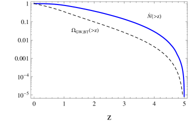
Figure 1: Fraction of the observed merger rate ${\dot{N}}_{T}$ and the foreground amplitude $\Omega_{GW,BT}$ by NS+NSs more distant than a given redshift. We plot numerical results for the fiducial merger rate $s(z)=s_{I}(z)$ (see also Cutler:2005qq ).

The correlation analysis is a powerful method to detect weak stochastic GW signals Flanagan:1993ix . In terms of the normalized energy density $\Omega_{GW}$, we can, in principle, realize a factor of $\sim SN^{-1}(fT_{obs})^{1/2}$ ($SN$, the signal-to-noise ratio for detection; $T_{obs}$, observation period) better sensitivity, compared with the sensitivity $\Omega_{GW,detector}\sim 10^{-14}$ directly corresponding to the noise spectrum of BBO. With BBO/DECIGO and an observational period of $T_{obs}\sim 10$yr, the limiting sensitivity of the correlation analysis to a stochastic GW background is $\Omega_{GW,lim}\sim 10^{-16}$ around the optimal frequency $f\sim 0.3$Hz where we are free from the potential foreground by double white-dwarf binaries Seto:2005qy . This limiting sensitivity $\Omega_{GW,lim}$ is a not a simple power-law function of GW frequency $f$, because of the shapes of the overlap reduction function (for definition see e.g. Flanagan:1993ix ) and the detector noise spectrum. In order to fully exploit the potential specification of the proposed detectors and to pursue a weak primordial GW background down to their limiting sensitivity $\Omega_{GW,lim}\sim 10^{-16}$, we need to subtract the NS+NS foreground and make the residual smaller by at least a factor of

$$\frac{\Omega_{GW,lim}}{\Omega_{GW,BT}}\sim 5.6\times 10^{-5}\left(\frac{{\dot{n}}_{0}}{10^{-7}{\rm Mpc^{-3}yr^{-1}}}\right)^{-1}$$ (18)

around the optimal frequency of BBO/DECIGO $f\sim 0.3$Hz, by identifying NS+NSs up to their highest redshift. Note again that the above target residual level ($\Omega_{GW,lim}\sim 10^{-16}$) is much lower than the detector noise level (corresponding to $\Omega_{GW,detector}\sim 10^{-14}$). In Fig. 1, we show the fraction of the foreground $\Omega_{GW,BT}$ made by binaries more distant than a given redshift $z$.

Now we discuss the observation of chirping GWs from individual NS+NSs with BBO/DECIGO. Here, we study typical binaries using the unperturbed GW amplitudes. The lensed signals would be analyzed in Sec.III. In what follows, we neglect dependence on sky positions and polarization angles of binaries, and we apply the averaged response of detectors with respect to these parameters. This is because multiple detectors with different orientations would be used for BBO/DECIGO bbo ; Kawamura , and we can expect a relatively weak dependence of signal-to-noise ratio on the direction and polarization angles, owing to an effective averaging effect (see e.g. Seto:2004ji for averaging on the direction angles). This prescription simplifies our analysis (see also Cutler:2005qq ). But, with only one detector, more detailed studies would be required for sources with short signal durations (e.g. 1 week).

We can evaluate the amplitudes of the two polarization modes of a binary with the quadrupole formula. In the frequency domain and in the principle polarization coordinate, their explicit forms for a circular orbit are given by Thorne_K:1987

$$(h_{+},h_{\times})=\sqrt{\frac{5}{96}}\frac{\pi^{-2/3}G^{5/6}M_{c}^{5/6}f^{-7/6}}{(1+z)^{1/6}c^{3/2}r(z)}(1+u^{2},2u).$$ (19)

Here, we defined the geometrical parameter $u\equiv\cos I$ using the inclination angle $I$. A face-on (edge-on) binary has $I=0$ ($I=\pm\pi/2$ respectively). Meanwhile, for a NS+NS at frequency $f$, the time $T_{GW}$ before the merger is given by

$$T_{GW}\sim 1\left(\frac{f}{0.2{\rm Hz}}\right)^{-8/3}(1+z)^{-5/3}~{}{\rm yr},$$ (20)

and smaller than planned operation period of BBO/DECIGO.

For signal analysis of each binary, we assume that, with some workable methods, the residual foreground would eventually become smaller than the detector noise after subtractions of binary signals Cutler:2005qq . This justifies our treatment below in which we consider only the detector noises for estimating the signal-to-noise ratio of individual binary. Note that this is a much weaker assumption compared with the previous requirement for realizing the ultimate sensitivity for detecting the weak GW background with correlation analysis. We put the signal-to-noise ratio $\rho(z,u)$ of unperturbed chirping GW from a NS+NS at a redshift $z$ as follows

$$\rho(z,u)=\frac{BM_{c}^{5/6}F(u)^{1/2}}{(1+z)^{1/6}r(z)}$$ (21)

with a function $F(u)\equiv 1+6u^{2}+u^{4}$ (see Cutler:2005qq ). Here, $B$ is a constant determined by the noise spectrum of the detectors. Given the designed sensitivity of BBO, we fix the parameter $B$ so that the signal-to-noise ratio becomes $\rho(z=5,u=0)=40$ to match Cutler:2005qq . For other redshifts, we have $\rho(z=10,0)=30,\rho(3,0)=52$ and $\rho(1,0)=110$. We also have $\rho(z,1)/\rho(z,0)=(F(1)/F(0))^{1/2}=2\sqrt{2}$ for dependence on the inclination angle, as commented in Sec. 1. For the fiducial merger model $s=s_{I}(z)$ with a realistic normalization ${\dot{n}}_{0}\lesssim 10^{-6}{\rm Mpc^{-3}yr^{-1}}$, Cutler and Harms Cutler:2005qq showed that the designed sensitivity of BBO [corresponding to $\rho(z=5,0)=40$] would enable us to detect all of the (unlensed) binaries and make their residual below the limiting sensitivity $\Omega_{GW,lim}\sim 10^{-16}$.

For an evaluation later in Sec. IV, we also define the mean signal-to-noise ratios by

$${\bar{\rho}}\equiv\frac{4\pi c\int_{0}^{\infty}dz\int_{0}^{1}du\frac{r(z)^{2}{\dot{n}}(z)}{(1+z)H(z)}\rho(z,u)^{2}}{{\dot{N}}_{T}}.$$ (22)

We numerically evaluated this expression and obtained ${\bar{\rho}}=187$ for $s=s_{I}$ and ${\bar{\rho}}=161$ for $s=s_{II}$.

III demagnified GW signals

III.1 Lensing Probability

Strong gravitational lensing produces multiple signals for an intrinsically single event lens . In this subsection, we discuss the faint end of GW signals caused by strong lensing. For the density profile of the lens objects, we use the SIS that captures lens structures well at the scales relevant for the strong lensing events lens . Here, we do not include detailed effects such as the external tidal shear field or the ellipticity of lenses, which cause minor corrections for the strong lensing probability itself (see e.g. Huterer:2004jh , and discussions on the quadruple lenses therein).

The explicit form of the SIS density profile $\frac{v^{2}}{3\pi GR^{2}}$ ($R$: the radial coordinate) is characterized by the one-dimensional velocity dispersion $v$. We further introduce the unperturbed angular diameter distances $D_{os}$, $D_{ol}$ and $D_{ls}$ between the observer-source, observer-lens and lens-source respectively. For example, the distance $D_{ol}$ is given by

$$D_{ol}=\frac{r(z_{l})}{1+z_{l}}$$ (23)

with the comoving distance $r(z)$ defined in Eq.(9). In order to study lens mapping, we define the characteristic angle

$$\theta_{d}\equiv\frac{4\pi v^{2}D_{ls}}{c^{2}D_{os}}$$ (24)

and use the two-dimensional coordinate ${y}$ for the source plane normalized with the length unit $\theta_{d}D_{os}$. We also introduce the coordinate ${x}$ for the lens plane normalized with the length $\theta_{d}D_{ol}$. The origin of these two coordinates are fixed at the direction of the lens center from the observer. Then the lens equation for the SIS model is given by lens

$$\mbox{\boldmath${y}$}={\mbox{\boldmath${x}$}}-{\mbox{\boldmath${x}$}}/|{\mbox{\boldmath${x}$}}|.$$ (25)

Because of the apparent symmetry around the lens center, the lens mapping between ${x}$ and ${y}$ is essentially one-dimensional correspondence on lines passing their origins. The lens equation (25) has two solutions

$$x_{\pm}=y\pm 1$$ (26)

for a small impact parameter at $0\leq y<1$, and one solution

$$x=y+1$$ (27)

for a large impact parameter at $y\geq 1$.

The amplification factor $A$ of gravitational lensing is evaluated with the Jacobian of the mapping and given by

$$A=\sqrt{\left|\frac{x}{y}\frac{dx}{dy}\right|}.$$ (28)

For the two solutions $x_{\pm}$, the amplification (28) becomes

$$A_{+}=\sqrt{1/y+1},~{}~{}~{}A_{-}=\sqrt{1/y-1}.$$ (29)

Comparing these two signals, the second one corresponds to the inner, fainter signal with a later arrival time. Note that the amplification $A$ is defined by the square root of the magnification $\mu$ which is often used in the literature on gravitational lensing of electro-magnetic waves lens . Our definition here reflects the important fact that, for detecting GW from a binary, we directly observe the waveform itself ($\propto h$), not its energy ($\propto h^{2}$).

In contrast to the identity $A_{+}>1$, the fainter counterpart $A_{-}$ approaches zero in the limit $y\to 1$ (from below). Since we are interested in weak GW signals that might be undetectable, we mainly study the fainter one $A_{-}$ rather than the brighter one $A_{+}$. The signal-to-noise ratio of a demagnified signal is expressed as $A_{-}\rho(z,u)$.

At $y\sim 1$, the time delay between two signals is given by lens

$$\Delta t \sim 32\pi^{2}\left(\frac{v}{c}\right)^{4}\frac{D_{ol}D_{ls}}{cD_{os}}(1+z_{l})$$

$$\sim 8.6\times 10^{6}\left(\frac{v}{210\rm km/sec}\right)^{4}\left(\frac{D_{ol}D_{ls}D_{os}^{-1}(1+z_{l})}{\rm 1Gpc}\right){\rm sec}.$$

For a typical velocity dispersion $v$ of a lens object, we have the relation $f\Delta t\gtrsim 10^{6}\gg 1$ around the optimal frequency of BBO/DECIGO $f\sim 0.3$Hz. Therefore, in the present situation, the geometrical optics approximation would work well Takahashi:2003ix , and the strongly-lensed two signals would be observed as two distinct chirping waveforms. But it might be interesting to analyze potential wave effects (e.g. in relation to substructure of lenses) Takahashi:2003ix . For the SIS model, the separation angle $\Delta\theta$ between the two images is given by lens

$$\Delta\theta=2\theta_{d}\sim 2.4"\left(\frac{D_{ls}}{D_{os}}\right)\left(\frac{v}{\rm 210km/sec}\right)^{2}.$$ (30)

With the expression for the characteristic angle $\theta_{d}$ defined in Eq.(24), the probability of the strong lensing event for a source at redshift $z_{s}$ is given by

$$P_{d}(z_{s})=\int_{0}^{z_{s}}dz_{l}\int_{0}^{\infty}dv\frac{dN}{dv}\frac{16\pi^{3}c^{-3}v^{4}(1+z_{l})^{2}D_{ls}^{2}D_{ol}^{2}}{H(z_{l})D_{os}^{2}},$$ (31)

where $\frac{dN}{dv}$ is the distribution function for velocity dispersions of lens objects. In this paper, we use the following model

$$v\frac{dN}{dv}=\frac{\phi_{*}\beta}{\Gamma(\alpha/\beta)}\left(\frac{v}{v_{*}}\right)^{\alpha}\exp\left[-\left(\frac{v}{v_{*}}\right)^{\beta}\right]$$ (32)

characterized by parameters $\phi_{*}=4.1\times 10^{-3}h^{3}{\rm Mpc^{-3}}$, $v_{*}=88.8{\rm km~{}sec^{-1}}$, $\alpha=6.5$ and $\beta=1.93$ Oguri:2007sv . We neglect the cosmological evolution of this function. This is partially supported by actual lensing observation up to $z_{s}\sim 1$. Our main results [e.g. Eqs.(42) and (46)] change only slightly, for an evolutionary model with the following set of parameters analyzed in Oguri:2007sv

$$\phi_{*}(z_{l})=\phi_{*}(1+z_{l})^{-0.229},~{}~{}~{}\sigma_{*}(z_{l})=\sigma_{*}(1+z_{l})^{-0.01}.$$ (33)

The product $v^{4}dN/dv$ is relevant for the lensing probability and also for the distribution of time delays. It becomes maximum at $v=2.4\sigma_{*}=210$km/sec and steeply declines at large $v$, as expected from the fraction

$$\frac{\int_{4\sigma_{*}}^{\infty}dvv^{4}dN/dv}{\int_{0}^{\infty}dvv^{4}dN/dv}\sim 10^{-4}.$$ (34)

Even for a high-redshift source $z_{s}\sim 5$, the redshift integral (31) has dominant contribution around $z_{l}\sim 1$. In Fig. 2, we present the lensing probability $P_{d}(z)$, as a function of the source redshift $z$.

On the source plane, the demagnification $A_{-}(<1)$ corresponds to the normalized radial coordinate as

$$y=\frac{1}{A_{-}^{2}+1}.$$ (35)

Therefore, the probability that a source at a redshift $z$ has a demagnification in the range $[A_{-},A_{-}+dA_{-}]$, is given by

$$\frac{dP}{dA_{-}}dA_{-}=P_{d}(z)\frac{4A_{-}}{(A_{-}^{2}+1)^{3}}dA_{-}.$$ (36)

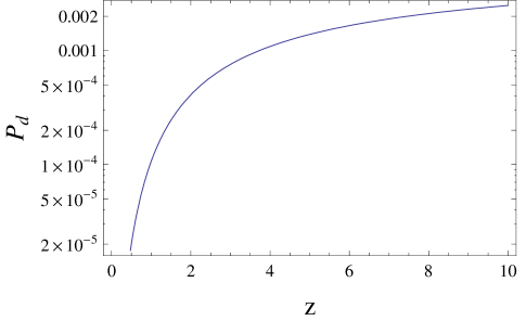
Figure 2: Probability of having multiple lensed images as a function of the source redshift $z$. For the velocity distribution function $dN/dv$, we use the no-evolution model given by Eq.(32).

III.2 Undetectable Lensed Signals

In this subsection, we study the subtraction problem for lensed GWs emitted by cosmological NS+NSs. First we evaluate the event rate for strongly-lensed GWs. For binaries at redshift $z$, the fraction $R_{0}(z)$ of the strongly-lensed GWs coincides with the probability $P_{d}(z)$ given in Eq.(31) as

$$R_{0}(z)\equiv P_{d}(z).$$ (37)

Then the total merger rate of the lensed signals is written as

$${\dot{N}}_{L}\equiv 4\pi\int_{0}^{\infty}dz\frac{r(z)^{2}R_{0}(z){\dot{n}}(z)}{(1+z)H(z)}.$$ (38)

For the fiducial model $s=s_{I}(z)$, we numerically evaluated this expression and obtained the averaged lensing probability

$${\bar{P}}\equiv{\dot{N}}_{L}/{\dot{N}}_{T}=3.7\times 10^{-4}$$ (39)

or equivalently

$${\dot{N}}_{L}=40\left(\frac{{\dot{n}}_{0}}{\rm 10^{-7}Mpc^{-3}yr^{-1}}\right){\rm yr^{-1}}.$$ (40)

For the flat-rate model $s(z)=s_{II}(z)$, we have the ratio ${\dot{N}}_{L}/{\dot{N}}_{T}=8.6\times 10^{-4}$.

Next we discuss a demagnified GW signal whose signal-to-noise ratio $A_{-}\rho(z,u)$ is less than a detection threshold $\rho_{th}$. To begin with, we estimate the relevant value $\rho_{th}$, taking into account the observational situation of the two lensed signals. The typical time delay $\Delta t$ between the earlier bright signal with $A_{+}$ and the later faint one with $A_{-}$ is much less than the planned observational period $T_{obs}\sim 10$yr of BBO/DECIGO. Thus we mainly consider a scenario to search for the demagnified signals under the detection of the bright ones . Except for the coalescence time $t_{c}$, the fitting parameters of the normalized waveforms of the two lensed signals can be regarded as almost identical, and these parameters would be generally well determined with the bright first image. For example, with BBO, the typical size of the localization error-ellipsoids in the sky is $\sim 10"\times 10"$ for a NS+NS at $z\sim 5$ Cutler:2005qq . On the other hand, the characteristic image separation $\Delta\theta$ in Eq.(30) is several arcseconds. Therefore, directions of two lensed images would be fitted by the same parameter for a NS+NS at $z\sim 5$. But, for a NS+NS at low redshift, the second image could get out of the error-ellipsoid of the brighter image.

The similarities of fitting parameters would significantly ease the detection of the demagnified one with the matched filtering method, compared with its single detection for which we need $10^{30}$-$10^{36}$ templates to make a full coherent signal integration. Even with the estimated computational power available at the era of BBO/DECIGO, we cannot make so many templates, and we need to use a suboptimal detection method which requires a higher detection threshold ($\rho_{cr}>20$ see Cutler:2005qq ) than the (optimal) coherent integration. Therefore, the information of the brighter signal considerably decreases the detection threshold $\rho_{th}$ for a lensed second signal, compared with its single detection. For the typical number of templates $n_{t_{c}}\sim 10^{7}$-$10^{8}$ estimated from the binning of the coalescence time $t_{c}$ of the faint image, the required condition for the threshold $\rho_{th}$ with respect to a false alarm rate $f_{r}$ is given as Cutler:2005qq

$$f_{r}\sim N_{t_{c}}{\rm erf}(\rho_{th}/\sqrt{2}),$$ (41)

and we have the solution $\rho_{th}\sim 6.5$ for $f_{r}\sim 0.01$. Including a safety factor (e.g. potential resampling of other fitting parameters around the bright signal), we take $\rho_{th}=10$ as a standard value for detecting the faint second image. For a reference we also use a pessimistic value $\rho_{th}\sim 20$ in the analyses below Cutler:2005qq . The results for this higher value would also provide us with an insight about the stand-alone analysis for a demagnified signal without using the information of the associated brighter one.

Here, we briefly comment on the identification of lensed pairs. The order-of-magnitude estimation for the required numbers of binning for the redshifted chirp mass $M_{c}(1+z)$ is $\sim 10^{8}$, which is much larger than the relevant numbers of NS+NSs $\sim 10^{5}$ Cutler:2005qq . In addition, given the good localization in the sky, directions of binaries would also become useful information to identify a lensed pair. Therefore it is unlikely to misidentify GWs from two different NS+NSs as a lensed pair. Although our aim in this paper is not to discuss further scientific possibilities with identified lensed pairs, such studies would be also interesting Cutler:2009qv ; Itoh:2009iy .

Now we statistically study the demagnified GW signals that are below the detection threshold with $A_{-}\rho(z,u)<\rho_{th}$. The fraction of the number of undetectable signals at a redshift $z$ is given as follows;

$$R_{1}(z)\equiv\frac{\int_{0}^{\infty}dA_{-}\int_{0}^{1}du\frac{dP}{dA_{-}}\Theta(\rho_{th}-A_{-}\rho(z,u))}{\int_{0}^{1}du}.$$ (42)

Here $\Theta(x)$ is the step function. In Fig. 3, we plot the function $R_{1}(z)$ for two choices: $\rho_{th}=10$ and 20. At the small amplification regime $A_{-}\ll 1$, the probability of having an amplification less than a given value $A_{-}$ is proportional to $A_{-}^{2}$ [see Eq.(36)], and we have an asymptotic scaling relation $R_{1}\propto\rho_{th}^{2}$. But we should be careful to note that this scaling relation depends on the details of the lensing profile and is not universal. The event rate ${\dot{N}}_{U}$ ($U$, undetectable) of the undetectable signals is evaluated as in Eq.(38) and we have

$${\dot{N}}_{U}=4\pi\int_{0}^{\infty}dz\frac{r(z)^{2}R_{1}(z){\dot{n}}(z)}{(1+z)H(z)}.$$ (43)

For the fiducial model $s(z)=s_{I}(z)$ and the threshold $\rho_{th}=10$, we numerically obtained the result

$${\dot{N}}_{U}=1.1\left(\frac{{\dot{n}}_{0}}{10^{-7}{\rm Mpc^{-3}yr^{-1}}}\right){\rm yr^{-1}},$$ (44)

or equivalently

$${\dot{N}}_{U}/{\dot{N}}_{T}=1.1\times 10^{-5}.$$ (45)

With the higher threshold $\rho_{th}=20$, the ratio becomes ${\dot{N}}_{U}/{\dot{N}}_{T}=3.9\times 10^{-5}$.

We move to evaluate the energy spectrum of the GW foreground made by undetectable binary signals with $A_{-}\rho(z,u)<\rho_{th}$. Here we introduce the factor $R_{2}(z)$ as the fraction of the GW energy due to the undetectable signals at redshift $z$ relative to the total binaries at the redshift. Summing up the contribution of undetectable ones, the factor $R_{2}(z)$ is formally given by

$$R_{2}(z)\equiv\frac{\int dA_{-}\int_{0}^{1}du\frac{dP}{dA_{-}}\Theta(\rho_{th}-A_{-}\rho(z,u))\left\{A_{-}\rho(z,u)\right\}^{2}}{\int_{0}^{1}du\rho(z,u)^{2}}.$$ (46)

In Fig. 3 we provide the function $R_{2}(z)$ for two thresholds $\rho_{th}=10$ and 20. In the present case, we can derive the asymptotic behavior $R_{2}\propto\rho_{th}^{4}$ for the SIS profile, after a simple consideration on the factors in the numerator of Eq.(46).

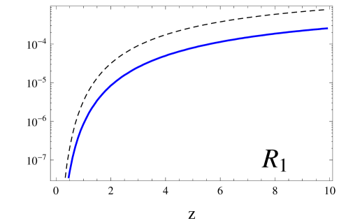
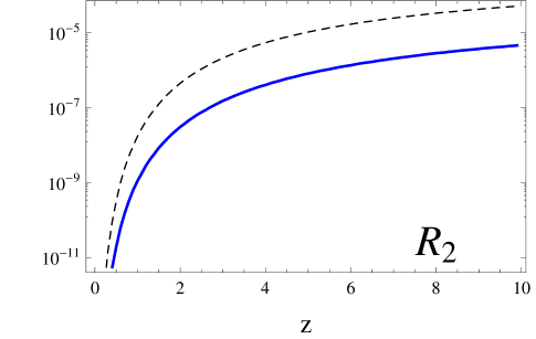
Figure 3: Relative contributions of the undetectable GW signals from NS+NSs at redshift $z$. The BBO noise curve is assumed with two choices of the detection threshold $\rho_{th}$ (dashed curve: $\rho_{th}=20$ and solid curve: $\rho_{th}=10$). Left panel: the number fraction $R_{1}(z)$ of the undetectable signals. Right panel: the fraction $R_{2}(z)$ of the GW energy density due to the undetected NS+NSs.

With the fraction $R_{2}(z)$, the energy spectrum $\Omega_{GW,BU}$ of the undetectable demagnified ones is expressed as

$$\Omega_{GW,BU}\equiv\frac{8\pi^{5/3}M_{c}^{5/3}f^{2/3}}{9H_{0}^{2}}\int_{0}^{\infty}\frac{{\dot{n}}(z)R_{2}(z)}{(1+z)^{4/3}H(z)}.$$ (47)

With the fiducial model $s(z)=s_{I}(z)$, we numerically obtained $\Omega_{GW,BU}/\Omega_{GW,BT}=1.5\times 10^{-8}$ for $\rho_{th}=10$ and $\Omega_{GW,BU}/\Omega_{GW,BT}=2.1\times 10^{-7}$ for $\rho_{th}=20$. With $s(z)=s_{II}(z)$, we have $9.8\times 10^{-8}$ ($\rho_{th}=10$) and $1.2\times 10^{-6}$ ($\rho_{th}=20$). Compared with the ratio in $(\ref{tar})$, the undetectable GW foreground would be comfortably smaller than the limiting sensitivity $\Omega_{GW,lim}\sim 10^{-16}$ for the realistic normalization ${\dot{n}}_{0}\lesssim 10^{-6}{\rm Mpc^{-3}yr^{-1}}$.

IV discussions

So far, we have studied the demagnified GW signals with the SIS density profile. Although this lens model is quite simple, it has reproduced observational results (with electro-magnetic waves) of gravitational lensing fairly well lens . But one might think that this model has been discussed at the relatively high-amplification regime where observations can be performed more easily. In this respect, it might be reasonable to wonder whether the simple SIS model is also a useful tool to study the strong lensing effects at the low-amplification regime as discussed in this paper. One simple example highlighting the situation is about the central third images of strong lensing Rusin:2000mm ; Keeton:2002ed . A lensing galaxy could have a core structure around its center, instead of the power-law profile $\propto r^{-2}$ of the SIS model, and such a density profile can generate a very faint third image around the direction toward the center of the lens. However, observational analysis of the third images is known to be quite difficult, partly due to the faintness of the signals . In addition to this example, it should be mentioned that, compared with typical electro-magnetic wave observation, GWs are generally measured at much lower frequencies and could be more susceptible to the wave effects (e.g. by substructures) that could complicate the signal analysis Takahashi:2003ix . In relation to the foreground cleaning which is essential for directly detecting a GW background from inflation, further studies on the faint end of lensing amplification would be worthwhile beyond our simple treatment.

On a final note, we attempt a more robust approach to evaluate the strength of the foreground composed by residual GW signals from undetected binaries, without using details of the probability distribution (36) for the demagnification $A_{-}$. Here, we simply assume that, if GW is strongly lensed, then the total signal-to-noise ratio of its unsubtracted component would be less than the detection threshold $\rho_{th}$. We define the residual $\Omega_{GW,BS}$ ($S$; simplified) as the summation of these unsubtracted ones. Since we have the relations $\Omega_{GW,BT}\propto N_{T}{\bar{\rho}}^{2}$ and $\Omega_{GW,BS}\propto N_{L}{\rho_{th}}^{2}=N_{T}{\bar{P}}{\rho_{th}}^{2}$ (see Eq.(39)), we obtain

$$\frac{\Omega_{GW,BS}}{\Omega_{GW,BT}}={\bar{P}}\left(\frac{\rho_{th}}{\bar{\rho}}\right)^{2}.$$ (48)

We regard the amplitude $\Omega_{GW,BS}$ as a conservative upper bound for the potential foreground made by the undetected signals. With the numerical results presented so far, we can evaluate this ratio and obtain

$$\frac{\Omega_{GW,BS}}{\Omega_{GW,BT}}=1.1\times 10^{-6}\left(\frac{\rho_{th}}{10}\right)^{2}$$ (49)

for the fiducial model $s(z)=s_{I}(z)$ and $3.3\times 10^{-6}(\rho_{th}/10)^{2}$ for $s(z)=s_{II}(z)$. Therefore, unless the normalization ${\dot{n}}_{0}$ is relatively high ${\dot{n}}_{0}\gtrsim 10^{-6}{\rm Mpc^{-3}yr^{-1}}$, the upper limit $\Omega_{GW,BS}$ is smaller than the limiting sensitivity $\Omega_{GW,lim}$ [see Eq.(18)], and we expect that the residual foreground caused by demagnified signals would not be a fundamental problem to detect an inflation background of $\Omega_{GW}\gtrsim 10^{-16}$ with BBO and DECIGO.

The author would like to thank R. Takahashi for helpful discussions. This work was supported by Grants-in-Aid for Scientific Research of the Japanese Ministry of Education, Culture, Sports, Science, and Technology Grant No. 20740151.

References

- (1) M. Maggiore, Phys. Rept. 331, 283 (2000); B. Allen, arXiv:gr-qc/9604033.
- (2) U. Seljak and M. Zaldarriaga, Phys. Rev. Lett. 78, 2054 (1997); M. Kamionkowski, A. Kosowsky and A. Stebbins, Phys. Rev. Lett. 78, 2058 (1997).
- (3) E. S. Phinney et al. The Big Bang Observer, NASA Mission Concept Study (2003).
- (4) N. Seto, S. Kawamura and T. Nakamura, Phys. Rev. Lett. 87, 221103 (2001).
- (5) S. Kawamura et al. Class. Quant. Grav. 23, 125 (2006).
- (6) T. L. Smith, M. Kamionkowski and A. Cooray, Phys. Rev. D 73, 023504 (2006) [arXiv:astro-ph/0506422].
- (7) P. L. Bender et al. LISA Pre-Phase A Report, Second edition, July 1998.
- (8) A. J. Farmer and E. S. Phinney, Mon. Not. Roy. Astron. Soc. 346, 1197 (2003) [arXiv:astro-ph/0304393].
- (9) A. Buonanno, G. Sigl, G. G. Raffelt, H. T. Janka and E. Muller, Phys. Rev. D 72, 084001 (2005) [arXiv:astro-ph/0412277]; P. Sandick, K. A. Olive, F. Daigne and E. Vangioni, Phys. Rev. D 73, 104024 (2006) [arXiv:astro-ph/0603544]; Y. Suwa, T. Takiwaki, K. Kotake and K. Sato, Astrophys. J. 665, L43 (2007) [arXiv:0706.3495 [astro-ph]]; S. Marassi, R. Schneider and V. Ferrari, arXiv:0906.0461 [astro-ph.CO].
- (10) C. Cutler and J. Harms, Phys. Rev. D 73, 042001 (2006) [arXiv:gr-qc/0511092].
- (11) J. Harms, C. Mahrdt, M. Otto and M. Priess, Phys. Rev. D 77, 123010 (2008) [arXiv:0803.0226 [gr-qc]].
- (12) V. Kalogera et al., Astrophys. J. 601, L179 (2005).
- (13) P. Schenider, J. Ehlers and E. E. Falco, Gravitational Lenses (Springer, Berlin, 1992).
- (14) M. Bartelmann and P. Schneider, Phys. Rept. 340, 291 (2001) [arXiv:astro-ph/9912508].
- (15) C. Cutler and D. E. Holz, arXiv:0906.3752 [astro-ph.CO].
- (16) Y. Itoh, T. Futamase and M. Hattori, arXiv:0908.0186 [gr-qc].
- (17) A. J. Barber, P. A. Thomas, H. M. P. Couchman and C. J. Fluke, Mon. Not. Roy. Astron. Soc. 319, 267 (2000) [arXiv:astro-ph/0002437].
- (18) E. S. Phinney, arXiv:astro-ph/0108028.
- (19) E. E. Flanagan, Phys. Rev. D 48, 2389 (1993); B. Allen and J. D. Romano, Phys. Rev. D 59, 102001 (1999).
- (20) N. Seto, Phys. Rev. D 73, 063001 (2006) [arXiv:gr-qc/0510067]; V. Corbin and N. J. Cornish, Class. Quant. Grav. 23, 2435 (2006) [arXiv:gr-qc/0512039].
- (21) N. Seto, Phys. Rev. D 69, 123005 (2004) [arXiv:gr-qc/0403014].
- (22) N. Dalal, D. E. Holz, S. A. Hughes and B. Jain, Phys. Rev. D 74, 063006 (2006) [arXiv:astro-ph/0601275].
- (23) D. Huterer, C. R. Keeton and C. P. Ma, Astrophys. J. 624, 34 (2005) [arXiv:astro-ph/0405040].
- (24) R. Takahashi and T. Nakamura, Astrophys. J. 595, 1039 (2003) [arXiv:astro-ph/0305055].
- (25) M. Oguri et al., Astron. J. 135, 512 (2008) [arXiv:0708.0825 [astro-ph]].
- (26) D. Rusin and C. P. Ma, arXiv:astro-ph/0009079.
- (27) C. R. Keeton, Astrophys. J. 582, 17 (2003) [arXiv:astro-ph/0206243].