Dirac equation with ultraviolet cutoff and quantum walk

Abstract

The weak convergence theorems of the one- and two-dimensional simple quantum walks, SQW${}^{(d)},d=1,2$, show a striking contrast to the classical counterparts, the simple random walks, SRW^(d). In the SRW^(d), distribution of position ${\bf X}(t)$ of the particle starting from the origin converges to the Gaussian distribution in the diffusion scaling limit, in which the time scale $T$ and spatial scale $L$ both go to infinity with keeping the ratio $L/\sqrt{T}$ to be finite. On the other hand, in the SQW^(d), the ratio $L/T$ is kept to define the pseudovelocity ${\bf V}(t)={\bf X}(t)/t$, and then all joint moments of the components $V_{j}(t),1\leq j\leq d$, of ${\bf V}(t)$ converges in the $T=L\to\infty$ limit. The limit distributions have novel structures such that they are inverted-bell shaped and the supports of them are bounded. In the present paper we claim that these properties of the SQW^(d) can be explained by the theory of relativistic quantum mechanics. We show that the Dirac equation with a proper ultraviolet cutoff can provide a quantum walk model in three dimensions, where the walker has a four-component qubit. We clarify that the pseudovelocity ${\bf V}(t)$ of the quantum walker, which solves the Dirac equation, is identified with the relativistic velocity. Since the quantum walker should be a tardyon, not a tachyon, $|{\bf V}(t)|<c$, where $c$ is the speed of light, and this restriction (the causality) is the origin of the finiteness of supports of the limit distributions universally found in quantum walk models. By reducing the number of components of momentum in the Dirac equation, we obtain the limit distributions of pseudovelocities for the lower dimensional quantum walks. We show that the obtained limit distributions for the one- and two-dimensional systems have the common features with those of SQW⁽¹⁾ and SQW⁽²⁾.

I INTRODUCTION

The notion of quantization of random walks has been widely discussed ADZ93 ; Mey96 ; NV00 ; ABNVW01 ; TM02 ; Kon02 ; Kem03 ; Amb03 ; Ken06 ; BBCKPX08 and applications of quantum walk models have been studied, for example, in information theory Gro97 ; NC00 ; Amb04 and in solid-state physics OKAA05 . One of the new topics in the study of quantum walks is to discuss the relationship between quantum walk models and the relativistic quantum mechanics KFK05 ; Str06 ; BES07 ; Str07 . In the present paper, we concentrate on the weak limit theorem of pseudovelocity of quantum walk, which was first proved by Konno for the one-dimensional simple quantum walk Kon02 ; Kon05 and then has been obtained for other models GJS04 ; IKK04 ; MKK07 ; WKKK08 ; SK08 ; Kon09 , and connections between the solutions of the Dirac equations and the quantum walk models are reported.

Simple random walk (SRW) is a discrete-time stochastic process defined on a lattice such that particle hopping is allowed only between nearest neighbor sites at each time step. Let ${\bf Z}$ be the set of all integers, ${\bf Z}=\{\dots,-2,-1,0,1,2,3,\dots\}$. We consider the models on the $d$-dimensional hypercubic lattices ${\bf Z}^{d}=\{{\bf x}=(x_{1},\dots,x_{d}):x_{j}\in{\bf Z},1\leq j\leq d\}$. For each site in ${\bf Z}^{d}$, there are $2d$ nearest neighbor sites and we put $p_{j}$ be the probability that the particle hops to the $j$-th nearest neighbor site, $1\leq j\leq 2d$. The elementary process of the SRW^(d) is determined by a $2d$-component vector ${\bf p}=(p_{1},\dots,p_{d})$ satisfying the conditions $0\leq p_{j}\leq 1,1\leq j\leq 2d$, and $\sum_{j=1}^{2d}p_{j}=1$. In other words, if we prepare such a die that it has $2d$ faces and the $j$-th face appears with probability $p_{j},1\leq j\leq 2d$, in each casting, a path of the $d$-dimensional SRW (SRW^(d)) can be determined by a sequential random casting of this die.

The $d$-dimensional simple quantum walk, SQW^(d), is obtained by quantizing the SRW^(d). In the quantization, the die is replaced by a “quantum die”, which is expressed by a $2d\times 2d$ unitary matrix $A^{(d)}\in{\rm U}(2d)$. In the Fourier space, the nearest neighbor hopping is also described by using a $2d\times 2d$ unitary matrix representing a shift operator, which is diagonal

$$S^{(d)}({\bf k})={\rm diag}\Big{[}e^{{\rm i}k_{1}},e^{-{\rm i}k_{1}},\dots,e^{{\rm i}k_{d}},e^{-{\rm i}k_{d}}\Big{]},$$ (1)

where ${\rm i}=\sqrt{-1}$ and $k_{j}\in(\pi,\pi]$ denotes the $j$-th component of the wave number vector ${\bf k}$. The dynamics of the SQW^(d) at each time step is then determined by the unitary matrix

$$V^{(d)}({\bf k})=S^{(d)}({\bf k})A^{(d)},\quad{\bf k}\in(-\pi,\pi]^{d}.$$ (2)

The important consequence of this quantization is that the state of the particle (quantum walker) at each time should be represented by a $2d$-component vector-valued wave function, to which the $2d\times 2d$ unitary matrix (2) is operated. We assume that there are only one quantum walker at the origin $O$ at time $t=0$. We let the walker have an initial $2d$-component qubit ${\bf q}=(q_{1},q_{2},\cdots,q_{2d})$ with $q_{j}\in{\bf C},1\leq j\leq 2d$ and $\sum_{j=1}^{2d}|q_{j}|^{2}=1$. That is, in the ${\bf k}$-space the initial wave function is independent of ${\bf k}$ and simply given by

$$\widehat{\Psi}({\bf k},0)=\widehat{\Psi}_{0}\equiv{{}^{\rm t}}(\begin{array}[]{cccc}q_{1}&q_{2}&\cdots&q_{2d}\end{array}),$$ (3)

where the left-superscript ${\rm t}$ means the transpose of the matrix. The wave function of the walker at time $t\in{\bf N}_{0}\equiv\{0,1,2,3,\dots\}$ is given in the ${\bf k}$-space and in the real space ${\bf R}^{d}$ by

$$\widehat{\Psi}({\bf k},t)=[V^{(d)}({\bf k})]^{t}\widehat{\Psi}_{0}$$ (4)

and

$$\Psi({\bf x},t)=\prod_{j=1}^{d}\int_{-\pi}^{\pi}\frac{dk_{j}}{2\pi}e^{{\rm i}{\bf k}\cdot{\bf x}}\widehat{\Psi}({\bf k},t),$$ (5)

respectively, where ${\bf k}\cdot{\bf x}=\sum_{j=1}^{d}k_{j}x_{j}$. The probability that the quantum walker is observed at site ${\bf x}\in{\bf Z}^{d}$ at time $t$ is given by

$$P({\bf x},t)=||\Psi({\bf x},t)||^{2}\equiv\Psi^{\dagger}({\bf x},t)\Psi({\bf x},t),$$ (6)

where $\Psi^{\dagger}({\bf x},t)={{}^{\rm t}}\overline{\Psi}({\bf x},t)$ denotes the Hermitian conjugate of $\Psi({\bf x},t)$. In this paper $\bar{z}$ denotes the complex conjugate of $z\in{\bf C}$. Let ${\bf X}(t)=(X_{1}(t),X_{2}(t),\dots,X_{d}(t))$ be the position of the quantum walker at time $t$, whose probability distribution is given by (6). The joint moment of the components $X_{j}(t),1\leq j\leq d$, of ${\bf X}(t)$ is then obtained by KFK05

$$\left\langle\prod_{j=1}^{d}(X_{j}(t))^{\alpha_{j}}\right\rangle \equiv \sum_{{\bf x}\in{\bf Z}^{d}}\prod_{j=1}^{d}x_{j}^{\alpha_{j}}P({\bf x},t)$$ (7)

$$= \prod_{j=1}^{d}\int_{-\pi}^{\pi}\frac{dk_{j}}{2\pi}\widehat{\Psi}^{\dagger}({\bf k},t)\prod_{j=1}^{d}\left({\rm i}\frac{\partial}{\partial k_{j}}\right)^{\alpha_{j}}\widehat{\Psi}({\bf k},t)$$

for any $\alpha_{j}\in{\bf N}_{0},1\leq j\leq d$.

The unitarity of the time-evolution operator (2) implies that in principle we are not able to find any convergence property of wave function $\Psi({\bf x},t)$ nor of the probability distribution $P({\bf x},t)$ in the long-time limit $t\to\infty$ in the SQW^(d). It presents a striking contrast to the classical stochastic processes, SRW^(d), which will generally converge to diffusion particle systems in the long-time $T\to\infty$ and large-scale $L\to\infty$ limit with the diffusion scaling $L/\sqrt{T}=$ const., and probability laws of the diffusion particle systems are described by using the Gaussian distribution functions. Konno Kon02 ; Kon05 discovered, however, that in the one-dimensional model, SQW⁽¹⁾, if we consider the pseudovelocity defined by

$$V_{1}(t)=\frac{X_{1}(t)}{t},$$ (8)

instead of the position $X_{1}(t)$ or the usual velocity $dX_{1}(t)/dt$, it does converge in a weak sense such that any moment of $V_{1}(t)$ converges to a moment of a continuous random variable as $t\to\infty$, whose distribution is given by a novel probability density function $\mu^{(1)}$. That is, Konno’s weak convergence theorem is given as follows Kon02 ; Kon05 . Consider the SQW⁽¹⁾ model driven by the quantum die

$$A^{(1)}=\left(\begin{array}[]{cc}a&b\cr-\overline{b}&\overline{a}\end{array}\right)\in{\rm U}(2),\quad a,b\in{\bf C},\quad|a|^{2}+|b|^{2}=1,$$ (9)

where the initial qubit of the walker is ${\bf q}=(q_{1},q_{2})$. Then for any $\alpha_{1}\in{\bf N}_{0}$

$$\lim_{t\to\infty}\Big{\langle}V_{1}(t)^{\alpha_{1}}\Big{\rangle}=\int_{-\infty}^{\infty}dv_{1}\,v_{1}^{\alpha_{1}}\nu^{(1)}(v_{1};A^{(1)},{\bf q}),$$ (10)

where

$$\nu^{(1)}(v_{1};A^{(1)},{\bf q})=\mu^{(1)}(v_{1};|a|){\cal M}^{(1)}(A^{(1)},{\bf q})$$ (11)

with

$$\mu^{(1)}(v_{1};|a|)=\frac{\sqrt{1-|a|^{2}}}{\pi(1-v_{1}^{2})\sqrt{|a|^{2}-v_{1}^{2}}}{\bf 1}(|v_{1}|<|a|),$$ (12)

$${\cal M}^{(1)}(A^{(1)},{\bf q})=1-\left(|q_{1}|^{2}-|q_{2}|^{2}+\frac{q_{1}\overline{q}_{2}a\overline{b}+\overline{q}_{1}q_{2}\overline{a}b}{|a|^{2}}\right).$$ (13)

Here ${\bf 1}(\omega)$ denotes the indicator function of a condition $\omega$; ${\bf 1}(\omega)=1$ if $\omega$ is satisfied and ${\bf 1}(\omega)=0$ otherwise. Figure 1 shows the density function $\mu^{(1)}(v_{1};|a|)$, when $a=1/\sqrt{2}$. The function $\mu^{(1)}$ is now called the Konno density function BBCKPX08 .

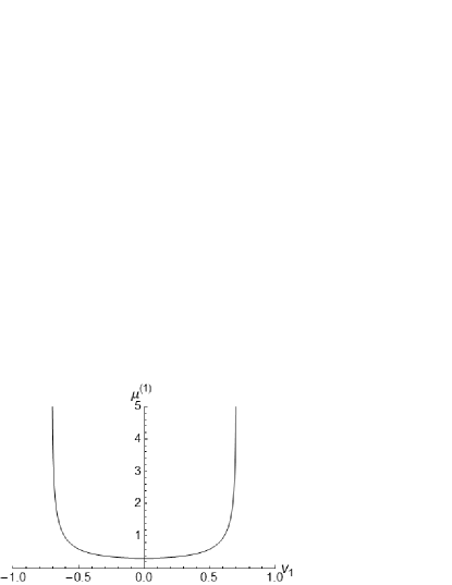
Figure 1: The one-dimensional density function $\mu^{(1)}(v_{1};|a|)$ of limit distribution of pseudovelocity for the SQW⁽¹⁾ (the Konno function), when $a=1/\sqrt{2}$.

Recently the weak convergence theorem of the two-component pseudovelocity

$${\bf V}(t)=(V_{1}(t),V_{2}(t))=\left(\frac{X_{1}(t)}{t},\frac{X_{2}(t)}{t}\right)$$ (14)

for the SQW⁽²⁾, where ${\bf X}(t)=(X_{1}(t),X_{2}(t))$ denotes the position of the walker, was also established WKKK08 , where the quantum die is parameterized by $p\in(0,1)$ as

$$A^{(2)}=\left(\begin{array}[]{cccc}-p&1-p&\sqrt{p(1-p)}&\sqrt{p(1-p)}\\ 1-p&-p&\sqrt{p(1-p)}&\sqrt{p(1-p)}\\ \sqrt{p(1-p)}&\sqrt{p(1-p)}&-(1-p)&p\\ \sqrt{p(1-p)}&\sqrt{p(1-p)}&p&-(1-p)\end{array}\right)\in{\rm U}(4).$$ (15)

For any $\alpha_{1},\alpha_{2}\in{\bf N}_{0}$,

$$\lim_{t\to\infty}\Big{\langle}V_{1}(t)^{\alpha_{1}}V_{2}(t)^{\alpha_{2}}\Big{\rangle}=\int_{-\infty}^{\infty}dv_{1}\int_{-\infty}^{\infty}dv_{2}\,v_{1}^{\alpha_{1}}v_{2}^{\alpha_{2}}\nu^{(2)}(v_{1},v_{2};A^{(2)},{\bf q})$$ (16)

where

$$\nu^{(2)}(v_{1},v_{2};A^{(2)},{\bf q})=\mu^{(2)}(v_{1},v_{2};p){\cal M}^{(2)}(v_{1},v_{2};A^{(2)},{\bf q})$$ (17)

with

$$\mu^{(2)}(v_{1},v_{2};p) = \frac{2}{\pi^{2}(v_{1}+v_{2}+1)(v_{1}-v_{2}+1)(v_{1}+v_{2}-1)(v_{1}-v_{2}-1)}$$ (18)

$$\qquad\times{\bf 1}(v_{1}^{2}/p+v_{2}^{2}/(1-p)<1).$$

The explicit expression of ${\cal M}^{(2)}(v_{1},v_{2};A^{(2)},{\bf q})$ as a function of ${\bf v}=(v_{1},v_{2})$, the parameter $p$ of the quantum die $A^{(2)}$, and the four-component initial qubit ${\bf q}=(q_{1},\dots,q_{4})$ is given in Sec.III.B in WKKK08 . Figure 2 shows the $p=1/2$ case of the density function $\mu^{(2)}$, which will be a two-dimensional extension of the Konno density function (12). The common feature of $\mu^{(1)}$ and $\mu^{(2)}$ is that they are inverted-bell shaped on bounded supports, an interval $(-a,a)$ and an elliptic region $\{(v_{1},v_{2}):v_{1}^{2}/p+v_{2}^{2}/(1-p)<1\}$, respectively, as shown in Figs.1 and 2. It is in a big contrast with the Gaussian distributions in $d=1$ and $d=2$, which are bell shaped with unbounded supports ${\bf R}$ and ${\bf R}^{2}$ describing the diffusion scaling limits of the SRW models, the one- and two-dimensional Brownian motions.

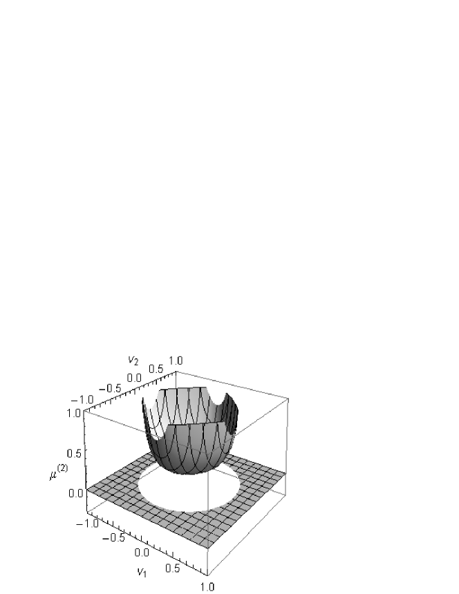
Figure 2: The two-dimensional density function $\mu^{(2)}(v_{1},v_{2};p)$ of limit distribution of pseudovelocity for the SQW⁽²⁾, when $p=1/2$.

The purpose of the present paper is to clarify the physical meaning of the pseudovelocities of quantum walkers, which can have limit distributions in the weak sense even in the quantum systems, and the origin of the inverted-bell shape of the limit distribution with bounded supports. Our argument is based on the resemblance between the quantum walk models and time-evolutions of multi-component wave functions in the relativistic quantum mechanics KFK05 ; Str06 ; BES07 ; Str07 . Since $V^{(d)}({\bf k})$ given by (2) is a unitary matrix, we can assign a Hermitian matrix ${\cal H}^{(d)}({\bf k})$ such that

$$V^{(d)}({\bf k})=e^{-{\rm i}{\cal H}^{(d)}({\bf k})/\hbar},$$ (19)

where $\hbar$ is a constant, the Planck constant divided by $2\pi$, and then the time evolution (4) of the SQW can be regarded as a solution of the equation

$${\rm i}\hbar\frac{\partial}{\partial t}\widehat{\Psi}({\bf k},t)={\cal H}^{(d)}({\bf k})\widehat{\Psi}({\bf k},t).$$ (20)

Here time $t$ is now thought to be a continuous variable in ${\bf R}$.

In an earlier paper KFK05 , a relation was reported between the SQW⁽¹⁾ model and the Weyl equation, which is given by (20) for the two component wave function, $\widehat{\Psi}({\bf k},t)={{}^{\rm t}}(\psi_{1}({\bf k},t)\,\psi_{2}({\bf k},t))$ with the Hamiltonian ${\cal H}^{(2)}({\bf k})=\mbox{\boldmath$\sigma$}\cdot{\bf k}$, where $\mbox{\boldmath$\sigma$}=(\sigma_{1},\sigma_{2},\sigma_{3})$ are the Pauli matrices,

$$\sigma_{1}=\left(\begin{array}[]{cc}0&1\cr 1&0\end{array}\right),\quad\sigma_{2}=\left(\begin{array}[]{cc}0&-{\rm i}\cr{\rm i}&0\end{array}\right),\quad\sigma_{3}=\left(\begin{array}[]{cc}1&0\cr 0&-1\end{array}\right).$$ (21)

Similarly, we expect a relation between the SQW⁽²⁾ and the Dirac equation, which is given in the form of (20) for the four-component wave function $\widehat{\Psi}({\bf k},t)={{}^{\rm t}}(\psi_{1}({\bf k},t)\,\dots,\psi_{4}({\bf k},t))$. Note that the Weyl equation and the Dirac equation are the time-evolution equations for massless and massive relativistic particles in quantum mechanics, both in the three-dimensional continuous space ${\bf R}^{3}$. So we have to note that the dimensionality $d$ of the SQW^(d) and that of the corresponding relativistic quantum mechanics is different from each other in general KFK05 . Moreover, we have to introduce a proper ultraviolet cutoff in the ${\bf k}$-space for the quantum mechanics, in order to establish the connection with the SQW^(d) as explained below in detail.

In Sec.II first we introduce the Dirac equation for a free particle in a usual way Dir58 ; BD64 ; IZ80 . Then we show that it can provide a model describing motion of a quantum walker having a four-component qubit by identifying the time-evolution matrix (2) with the Hamiltonian matrix for the Dirac equation explicitly. Then we study the long-time behavior of the moments of pseudovelocity for a free Dirac particle starting from the origin. Our initial state will be considered as an ideal limit of the highly localized state studied by Bracken, Flohr, and Melloy BFM05 . In this situation we clarify the fact that the pseudovelocity is exactly equal to the relativistic velocity. Since the Dirac particle as well as our quantum walker should be a tardyon, not a tachyon, its velocity is less than the speed of light $c$,

$$v=\sqrt{v_{1}^{2}+v_{2}^{2}+v_{3}^{2}}<c.$$ (22)

This is the physical origin of the finiteness of supports in the limit distributions of ${\bf V}(t)$ universally found in quantum walk models. In order to ensure the convergence of integrals giving joint moments of $V_{j}(t),1\leq j\leq 3,$ in $t\to\infty$, we have to introduce an ultraviolet cutoff in the theory, which will correspond to the fact that quantum walk models are defined on discrete spaces such as, lattices and trees. The introduction of an ultraviolet cutoff here will be equivalent with replacement of the delta-function-like initial state by a wave packet with a finite size as studied by Strauch Str07 for the one-dimensional systems (see Sec.III C). In Sec.III, we modify the Dirac equations by reducing the number of components of momentum to describing the quantum walk models in the dimensions lower than $d=3$. We list up the limit distributions of pseudovelocities of quantum walkers corresponding to these free Dirac particles in the dimensions $d=1$ and 2 with a proper ultraviolet cutoff. Then we compare the results with the limit distributions of the SQW^(d) with $d=1$ and 2 obtained in the previous papers Kon02 ; Kon05 ; KFK05 ; WKKK08 . Concluding remarks are given in Sec.IV associated with Appendix A.

II LIMIT DISTRIBUTION OF DIRAC EQUATION

II.1 Dirac equation as a quantum walk model

The Dirac equation for a free particle with the rest mass $m$ in the three-dimensional real space ${\bf R}^{3}$ is given by Dir58 ; BD64 ; IZ80

$${\rm i}\hbar\frac{\partial}{\partial t}\Psi({\bf x},t)=\widehat{\cal H}{\Psi}({\bf x},t)$$ (23)

for the four-component wave function $\Psi({\bf x},t)$ with the Hamiltonian operator

$$\widehat{\cal H}=\gamma_{4}\left(\sum_{k=1}^{3}c\hbar{\gamma_{k}}\frac{\partial}{\partial x_{k}}+mc^{2}\right),$$ (24)

where ${\gamma_{\nu}},\nu=1,2,3,4$, are the $4\times 4$ gamma matrices satisfying the algebra

$${\gamma_{\mu}}{\gamma_{\nu}}+{\gamma_{\nu}}{\gamma_{\mu}}=2\delta_{\mu\nu}I_{4},\quad\mu,\nu=1,2,3,4$$ (25)

with the $4\times 4$ unit matrix $I_{4}$. In the present paper, we fix the matrix representations as follows,

$$\gamma_{k}=\left(\begin{array}[]{cc}{\bf 0}&-{\rm i}\sigma_{k}\cr{\rm i}\sigma_{k}&{\bf 0}\end{array}\right),\quad k=1,2,3,\quad\gamma_{4}=\left(\begin{array}[]{cc}I&{\bf 0}\cr{\bf 0}&-I\end{array}\right),$$ (26)

where $\sigma_{k},k=1,2,3$, are the Pauli matrices given by (21) and $I$ and ${\bf 0}$ are the $2\times 2$ unit matrix and the $2\times 2$ zero matrix, respectively. From now on we consider the momentum ${\bf p}=(p_{1},p_{2},p_{3})$ of the particle, instead of the wave number vector ${\bf k}=(k_{1},k_{2},k_{3})$ of the wave function, where the de Broglie relation ${\bf p}=\hbar{\bf k}$ is established. The momentum ${\bf p}$ provides a good quantum number and the solution for a given momentum ${\bf p}$ is given by a plane wave,

$$\Psi_{{\bf p}}({\bf x},t)=e^{{\rm i}{\bf p}\cdot{\bf x}/\hbar-{\rm i}E(p)t/\hbar}u({\bf p}),$$ (27)

where

$$p=|{\bf p}|=\sqrt{p_{1}^{2}+p_{2}^{2}+p_{3}^{2}},\quad E(p)=\sqrt{(pc)^{2}+(mc^{2})^{2}},$$ (28)

and $u(p)$ is a four-component vector which satisfies the eigenvalue equation

$$E(p)u({\bf p})={\cal H}({\bf p})u({\bf p})$$ (29)

with the Hamiltonian matrix

$${\cal H}({\bf p})={\gamma_{4}}\left({\rm i}\sum_{k=1}^{3}c{\gamma_{k}}p_{k}+mc^{2}\right).$$ (30)

Then, in the momentum space, the wave function is given as

$$\widehat{\Psi}({\bf p},t)=e^{-{\rm i}{\cal H}({\bf p})t/\hbar}u({\bf p}).$$ (31)

The Hamiltonian matrix given by (30) can be diagonalized by the Foldy-Wouthuysen-Tani transformation FW50 ; Tani51 as follows:

$${\cal H}({\bf p})=U({\bf p})^{-1}E(p)\ \gamma_{4}U({\bf p})$$ (32)

with (28) and

$$U({\bf p}) = \frac{1}{\sqrt{2E(p)}}\left(\sqrt{E(p)+mc^{2}}\,I_{4}+{\rm i}\sum_{k=1}^{3}\frac{c\gamma_{k}p_{k}}{\sqrt{E(p)+mc^{2}}}\right)$$ (37)

$$= \frac{1}{\sqrt{2E(p)}}\left(\begin{array}[]{cccc}\sqrt{E(p)+mc^{2}}&0&\frac{cp_{3}}{\sqrt{E(p)+mc^{2}}}&\frac{c(p_{1}-{\rm i}p_{2})}{\sqrt{E(p)+mc^{2}}}\\ 0&\sqrt{E(p)+mc^{2}}&\frac{c(p_{1}+{\rm i}p_{2})}{\sqrt{E(p)+mc^{2}}}&\frac{-cp_{3}}{\sqrt{E(p)+mc^{2}}}\\ \frac{-cp_{3}}{\sqrt{E(p)+mc^{2}}}&\frac{-c(p_{1}-{\rm i}p_{2})}{\sqrt{E(p)+mc^{2}}}&\sqrt{E(p)+mc^{2}}&0\\ \frac{-c(p_{1}+{\rm i}p_{2})}{\sqrt{E(p)+mc^{2}}}&\frac{cp_{3}}{\sqrt{E(p)+mc^{2}}}&0&\sqrt{E(p)+mc^{2}}\end{array}\right).$$

Then we can see that

$$e^{-{\rm i}{\cal H}({\bf p})t/\hbar} = \sum_{n=0}^{\infty}\frac{1}{n!}\left(-{\rm i}\frac{{\cal H}({\bf p})}{\hbar}t\right)^{n}$$ (38)

$$= \sum_{n=0}^{\infty}\frac{1}{n!}\left(\frac{-{\rm i}t}{\hbar}\right)^{n}(U({\bf p})^{-1}E(p)\ \gamma_{4}U({\bf p}))^{n}$$

$$= U({\bf p})^{-1}\left[\sum_{n=0}^{\infty}\frac{1}{n!}\left(\frac{-{\rm i}t}{\hbar}\right)^{n}(E(p)\ \gamma_{4})^{n}\right]U({\bf p})$$

$$= \left[U({\bf p})^{-1}{\rm diag}\Big{[}e^{-{\rm i}E(p)/\hbar},e^{-{\rm i}E(p)/\hbar},e^{{\rm i}E(p)/\hbar},e^{{\rm i}E(p)/\hbar}\Big{]}U({\bf p})\right]^{t}.$$

It implies that the Dirac equation provides a quantum walk model, in which the walker is driven by the $4\times 4$ unitary matrix

$$V({\bf p})=U({\bf p})^{-1}{\rm diag}\Big{[}e^{-{\rm i}E(p)/\hbar},e^{-{\rm i}E(p)/\hbar},e^{{\rm i}E(p)/\hbar},e^{{\rm i}E(p)/\hbar}\Big{]}U({\bf p}),$$ (39)

where $U({\bf p})$ is given by (37).

II.2 Limit distribution of relativistic velocity

Let ${\bf X}(t)=(X_{1}(t),X_{2}(t),X_{3}(t))$ be the position of a free Dirac particle at time $t$ starting from the origin at time $t=0$. The joint moments of $X_{j}(t),1\leq j\leq 3$ are given by

$$\left\langle\prod_{j=1}^{3}X_{j}(t)^{\alpha_{j}}\right\rangle=\prod_{j=1}^{3}\int_{-\infty}^{\infty}\frac{dp_{j}}{2\pi\hbar}\,\widehat{\Psi}^{\dagger}({\bf p},t)\prod_{j=1}^{3}\left({\rm i}\hbar\frac{\partial}{\partial p_{j}}\right)^{\alpha_{j}}\widehat{\Psi}({\bf p},t).$$ (40)

Let ${\bf w}_{j}({\bf p})$ be the $j$-th row of the matrix $U({\bf p})$ given by (37), $1\leq j\leq 4$. We assume the initial state as

$$\widehat{\Psi}({\bf p},0)=\widehat{\Psi}_{0}\equiv{{}^{\rm t}}(\begin{array}[]{cccc}q_{1}&q_{2}&q_{3}&q_{4}\end{array}),$$ (41)

where $q_{j}\in{\bf C},1\leq j\leq 4$, are independent of ${\bf p}$ and $\sum_{j=1}^{4}|q_{j}|^{2}=1$. Then

$$\widehat{\Psi}({\bf p},t) = \left[U({\bf p})^{-1}{\rm diag}\Big{[}e^{-{\rm i}E(p)/\hbar},e^{-{\rm i}E(p)/\hbar},e^{{\rm i}E(p)/\hbar},e^{{\rm i}E(p)/\hbar}\Big{]}U({\bf p})\right]^{t}\widehat{\Psi}_{0}$$ (42)

$$= e^{-{\rm i}E(p)t/\hbar}\{{\bf w}_{1}({\bf p})C_{1}({\bf p})+{\bf w}_{2}({\bf p})C_{2}({\bf p})\}$$

$$+e^{{\rm i}E(p)t/\hbar}\{{\bf w}_{3}({\bf p})C_{3}({\bf p})+{\bf w}_{4}({\bf p})C_{4}({\bf p})\},$$

where $C_{j}({\bf p})\equiv[{\bf w}_{j}({\bf p})]^{\dagger}\widehat{\Psi}_{0},1\leq j\leq 4$.

For $\alpha_{j}\in{\bf N}\equiv\{1,2,\cdots\},1\leq j\leq 3$, we see GJS04

$$\prod_{j=1}^{3}\left({\rm i}\hbar\frac{\partial}{\partial p_{j}}\right)^{\alpha_{j}}\widehat{\Psi}({\bf p},t)$$ (43)

$$= \prod_{j=1}^{3}\left(\frac{\partial E(p)}{\partial p_{j}}\right)^{\alpha_{j}}e^{-{\rm i}E(p)t/\hbar}\Big{[}{\bf w}_{1}({\bf p})C_{1}({\bf p})+{\bf w}_{2}({\bf p})C_{2}({\bf p})\Big{]}{t}^{\sum_{j=1}^{3}\alpha_{j}}$$

$$+ \prod_{j=1}^{3}\left(-\frac{\partial E(p)}{\partial p_{j}}\right)^{\alpha_{j}}e^{{\rm i}E(p)t/\hbar}\Big{[}{\bf w}_{3}({\bf p})C_{3}({\bf p})+{\bf w}_{4}({\bf p})C_{4}({\bf p})\Big{]}{t}^{\sum_{j=1}^{3}\alpha_{j}}+{\cal O}\left(t^{\sum_{j=1}^{3}\alpha_{j}-1}\right).$$

Since $U({\bf p})$ is unitary, its row vectors $\{{\bf w}_{j}({\bf p})\}_{j=1}^{4}$ make a set of orthonormal vectors,

$${\bf w}_{j}^{{\dagger}}({\bf p}){\bf w}_{k}({\bf p})=\delta_{jk},\quad 1\leq j,k\leq 4.$$ (44)

Then we have

$$\widehat{\Psi}^{{\dagger}}({\bf p},t)\prod_{j=1}^{3}\left({\rm i}\hbar\frac{\partial}{\partial p_{j}}\right)^{\alpha_{j}}\widehat{\Psi}({\bf p},t)=\prod_{j=1}^{3}\left(\frac{\partial E(p)}{\partial p_{j}}\right)^{\alpha_{j}}$$

$$\qquad\times\left[|C_{1}({\bf p})|^{2}+|C_{2}({\bf p})|^{2}+(-1)^{\sum_{j=1}^{3}\alpha_{j}}\{|C_{3}({\bf p})|^{2}+|C_{4}({\bf p})|^{2}\}\right]{t}^{\sum_{j=1}^{3}\alpha_{j}}$$

$$\qquad\qquad+{\cal O}\left(t^{\sum_{j=1}^{3}\alpha_{j}-1}\right).$$ (45)

The pseudovelocity is defined as

$${\bf V}(t)=\left(\frac{X_{1}(t)}{t},\frac{X_{2}(t)}{t},\frac{X_{3}(t)}{t}\right),$$

and we obtain the long-time limit of the joint moments; for $\alpha_{j}\in{\bf N}_{0},1\leq j\leq 3$

$$\lim_{t\to\infty}\left\langle\prod_{j=1}^{3}V_{j}(t)^{\alpha_{j}}\right\rangle$$ (46)

$$= \prod_{j=1}^{3}\int_{-\infty}^{\infty}\frac{dp_{j}}{2\pi\hbar}\left[\{|C_{1}({\bf p})|^{2}+|C_{2}({\bf p})|^{2}\}+(-1)^{\sum_{j=1}^{3}\alpha_{j}}\{|C_{3}({\bf p})|^{2}+|C_{4}({\bf p})|^{2}\}\right]$$

$$\qquad\times\prod_{j=1}^{3}\left(\frac{\partial E(p)}{\partial p_{j}}\right)^{\alpha_{j}}.$$

Since $E(p)$ is the relativistic energy of the particle given by (28),

$$\frac{\partial E(p)}{\partial p_{j}}=c^{2}\frac{p_{j}}{E(p)},\quad j=1,2,3.$$ (47)

We change the variables of integrals in (46) from $p_{j}$’s to $v_{j}$’s by the transformation

$$v_{j}=c^{2}\frac{p_{j}}{E(p)},\quad j=1,2,3.$$ (48)

We can show that this map ${\bf p}\in{\bf R}^{3}\mapsto{\bf v}=(v_{1},v_{2},v_{3})$ is one-to-one and the image is an interior of a circle with radius $c$,

$$v_{x}^{2}+v_{y}^{2}+v_{z}^{2}<c^{2}.$$ (49)

Moreover, we find that the following relations are equivalent with (48),

$$p_{j}=\frac{mv_{j}}{\sqrt{1-v^{2}/c^{2}}},\quad j=1,2,3,$$ (50)

where $v=|{\bf v}|$. That is, ${\bf v}$ is the relativistic velocity of the particle. From this expression (50) we can readily calculate the Jacobian associated with the inverse map ${\bf v}\mapsto{\bf p}$,

$$J\equiv\det\left[\frac{\partial v_{j}}{\partial p_{k}}\right]_{1\leq j,k\leq 3}=c^{10}\frac{m^{2}}{E(p)^{5}}=\frac{1}{m^{3}}\left({1-\frac{v^{2}}{c^{2}}}\right)^{5/2}.$$

Associated with the change of variables, $C_{j}({\bf p})$’s are replaced by $\widehat{C}_{j}({\bf v})$’s and the integrals in (46) are rewritten as

$$\lim_{t\to\infty}\left\langle\prod_{j=1}^{3}V_{j}(t)^{\alpha_{j}}\right\rangle$$ (51)

$$= \prod_{j=1}^{3}\int_{-\infty}^{\infty}\frac{dv_{j}}{2\pi\hbar}\frac{1}{J}\left[\{|\widehat{C}_{1}({\bf v})|^{2}+|\widehat{C}_{2}({\bf v})|^{2}\}+(-1)^{\sum_{j=1}^{3}\alpha_{j}}\{|\widehat{C}_{3}({\bf v})|^{2}+|\widehat{C}_{4}({\bf v})|^{2}\}\right]$$

$$\qquad\qquad\times\prod_{j=1}^{3}v_{j}^{\alpha_{j}}{\bf 1}(v^{2}_{1}+v^{2}_{2}+v^{3}_{3}<c^{2})$$

$$= \prod_{j=1}^{3}\int_{-\infty}^{\infty}\frac{dv_{j}}{c}\prod_{j=1}^{3}v_{j}^{\alpha_{j}}\mu_{\rm Dirac}^{(3)}(v){\cal M}_{\rm Dirac}^{(3)}({\bf v};{\bf q})$$

for $\alpha_{j}\in{\bf N}_{0},1\leq j\leq 3$. Here

$$\mu_{\rm Dirac}^{(3)}(v)=\left(\frac{mc}{2\pi\hbar}\right)^{3}\frac{1}{(1-v^{2}/c^{2})^{5/2}}{\bf 1}(v<c),$$ (52)

and

$${\cal M}_{\rm Dirac}^{(3)}({\bf v};{\bf q})=1+\sum_{j=1}^{3}{\cal M}_{\rm Dirac}^{{}^{(3,j)}}({\bf q})v_{j}$$ (53)

with

$${\cal M}_{\rm Dirac}^{(3,1)}({\bf q})=2{\rm Re}(q_{1}\bar{q_{4}}+q_{2}\bar{q_{3}})\quad{\cal M}_{\rm Dirac}^{(3,2)}({\bf q})=2{\rm Im}(\bar{q_{1}}q_{4}-\bar{q_{2}}q_{3}),$$

$${\cal M}_{\rm Dirac}^{(3,3)}({\bf q})=2{\rm Re}(q_{1}\bar{q_{3}}-q_{2}\bar{q_{4}}),$$ (54)

where ${\rm Re}(z)$ and ${\rm Im}(z)$ denote the real part and the imaginary part of $z\in{\bf C}$, respectively.

II.3 Ultraviolet cutoff

The integrals

$$\prod_{j=1}^{3}\int_{-\infty}^{\infty}\frac{dv_{j}}{c}\prod_{j=1}^{3}v_{j}^{\alpha_{j}}\mu_{\rm Dirac}^{(3)}(v){\cal M}^{(3)}_{\rm Dirac}({\bf v};{\bf q}),\quad(\alpha_{1},\alpha_{2},\alpha_{3})\in{\bf N}_{0}^{3}$$ (55)

generally do not converge. In order to obtain finite values of physical quantities the momentum space should be restricted, and we set an ultraviolet cutoff by introducing a cutoff parameter $\lambda>0$ as

$$p=|{\bf p}|<\lambda.$$ (56)

The range of ${\bf v}=(v_{1},v_{2},v_{3})$ is then

$$v_{1}^{2}+v_{2}^{2}+v_{3}^{2}<\frac{\lambda^{2}c^{2}}{(mc)^{2}+\lambda^{2}}.$$ (57)

We can calculate the normalization constant for finite $\lambda$ as

$$\prod_{j=1}^{3}\int_{-\infty}^{\infty}\frac{dv_{j}}{c}\left(\frac{mc}{2\pi\hbar}\right)^{3}\frac{1}{(1-v^{2}/c^{2})^{5/2}}{\bf 1}\left(v<\sqrt{\frac{\lambda^{2}c^{2}}{(mc)^{2}+\lambda^{2}}}\right)=\frac{\lambda^{3}}{6\pi^{2}\hbar^{3}}.$$ (58)

Finally the distribution function is determined as

$$\mu_{\rm Dirac}^{(3)}(v;\lambda)=\frac{3}{4\pi}\left(\frac{mc}{\lambda}\right)^{3}\frac{1}{(1-v^{2}/c^{2})^{5/2}}{\bf 1}\left(v<\sqrt{\frac{\lambda^{2}c^{2}}{(mc)^{2}+\lambda^{2}}}\right).$$ (59)

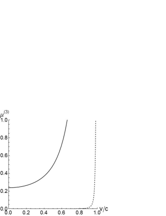
Figure 3: The dependence of $\mu_{\rm Dirac}^{(3)}$ on the magnitude $v$ of the pseudovelocity. The solid line for the cutoff parameter $\lambda/(mc)=1$, and the broken line for $\lambda/(mc)=10$, respectively.

We assume that $m$ is the rest mass of an electron. Figures 3 shows $\mu^{(3)}_{\rm Dirac}(v;\lambda)$ given by (59) as functions of $v=\sqrt{v_{1}^{2}+v_{2}^{2}+v_{3}^{2}}>0$ for the cutoff parameter $\lambda/(mc)=1$ (by the solid line) and 10 (by the broken line), respectively. They should be compared with Fig.1 in BFM05 . If $\lambda/(mc)\to\infty$, that is, the ultraviolet cutoff of the energy $\overline{E}=\lambda c$ becomes much greater than the rest mass energy $mc^{2}$ of the particle, $\mu_{\rm Dirac}^{(3)}(v;\lambda)\to\delta(v-c)$; the velocity of spreading of the Dirac particle outwards from the origin tends to be close to the speed of light $c$ BFM05 ; Str06 ; BES07 . Since quantum walk models are defined on lattices, an ultraviolet cutoff is naturally introduced so that $\lambda/(mc)=\overline{E}/(mc^{2})$ remains to be small, and thus the inverted-bell shaped distributions of pseudovelocities are universally observed.

The reason that the integrals for the moments (55) do not converge is due to our choice of initial state such that a Dirac particle is put at the origin at time $t=0$. It will be equivalent with setting the initial wave function be a delta function at the origin, which is not square-integrable. From this point of view, the introduction of ultraviolet cutoff in the present paper can be regarded as a modification of the initial state. In the paper Str07 , Strauch introduced a localization parameter $a$, which controls the effective size of the initial wave packet describing a Dirac particle and a quantum walker in the models. Dependence of the spatial distributions of wave packets in $t>0$ on the parameter $a$ and “initial qubit” was fully studied for the one-dimensional Dirac equation and the quantum walk models. We hope that the present paper will show the importance of his study to understand the relationship between the quantum walk models and the relativistic quantum mechanics also in the higher spatial-dimensions.

III LOWER DIMENSIONAL SYSTEMS

III.1 Two-dimensional system

We consider the Hamiltonian matrix

$${\cal H}({\bf p})=U({\bf p})^{-1}\sqrt{(pc)^{2}+(mc^{2})^{2}}\ \gamma_{4}U({\bf p})$$ (60)

with the two-component momentum ${\bf p}=(p_{1},p_{2})$, where $p=|{\bf p}|=\sqrt{p_{1}^{2}+p_{2}^{2}}$ and

$$U({\bf p})=\frac{1}{\sqrt{2E(p)}}\left(\sqrt{E(p)+mc^{2}}\,I_{4}+{\rm i}\sum_{k=1}^{2}\frac{c\gamma_{k}p_{k}}{\sqrt{E(p)+mc^{2}}}\right)$$

$$=\frac{1}{\sqrt{2E(p)}}\left(\begin{array}[]{cccc}\sqrt{E(p)+mc^{2}}&0&0&\frac{c(p_{1}-{\rm i}p_{2})}{\sqrt{E(p)+mc^{2}}}\\ 0&\sqrt{E(p)+mc^{2}}&\frac{c(p_{1}+{\rm i}p_{2})}{\sqrt{E(p)+mc^{2}}}&0\\ 0&\frac{-c(p_{1}-{\rm i}p_{2})}{\sqrt{E(p)+mc^{2}}}&\sqrt{E(p)+mc^{2}}&0\\ \frac{-c(p_{1}+{\rm i}p_{2})}{\sqrt{E(p)+mc^{2}}}&0&0&\sqrt{E(p)+mc^{2}}\end{array}\right)$$

with $E(p)=\sqrt{(pc)^{2}+(mc^{2})^{2}}$. Following the similar procedure to that given in Sec.II, we will obtain the following result under the ultraviolet cutoff (56) with a parameter $\lambda$; for $\alpha_{j}\in{\bf N}_{0},j=1,2$,

$$\lim_{t\to\infty}\left\langle\prod_{j=1}^{2}V_{j}(t)^{\alpha_{j}}\right\rangle_{\lambda}=\prod_{j=1}^{2}\int_{-\infty}^{\infty}\frac{dv_{j}}{c}\,\prod_{j=1}^{2}v_{j}^{\alpha_{j}}\nu_{\rm Dirac}^{(2)}({\bf v};\lambda,{\bf q})$$ (62)

with $v=\sqrt{v_{1}^{2}+v_{2}^{2}}$ and

$$\nu_{\rm Dirac}^{(2)}({\bf v};\lambda,{\bf q})=\mu_{\rm Dirac}^{(2)}(v;\lambda){\cal M}_{\rm Dirac}^{(2)}({\bf v};{\bf q}),$$ (63)

where

$$\mu_{\rm Dirac}^{(2)}(v;\lambda)=\frac{1}{\pi}\left(\frac{mc}{\lambda}\right)^{2}\frac{1}{(1-v^{2}/c^{2})^{2}}{\bf 1}\left(v<\sqrt{\frac{\lambda^{2}c^{2}}{(mc)^{2}+\lambda^{2}}}\right),$$ (64)

$${\cal M}_{\rm Dirac}^{(2)}({\bf v};{\bf q})=1+\sum_{j=1}^{2}{\cal M}_{\rm Dirac}^{(2,j)}({\bf q})v_{j}$$ (65)

with

$${\cal M}_{\rm Dirac}^{(2,1)}({\bf q})=2{\rm Re}(q_{1}\bar{q_{4}}+q_{2}\bar{q_{3}}),\quad{\cal M}_{\rm Dirac}^{(2,2)}({\bf q})=2{\rm Im}(\bar{q_{1}}q_{4}-\bar{q_{2}}q_{3}).$$ (66)

Figure 4 shows the comparison between (a) $\nu^{(2)}$ of the SQW⁽²⁾ given by (17) (see WKKK08 for detail), and (b) $\nu^{(2)}_{\rm Dirac}$ given by (63). Here we have chosen the parameters as (a) $p=1/2,{\bf q}=(1/2,-{\rm i}/2,-1/2,{\rm i}/2)$ and (b) $\lambda/(mc)=1,{\bf q}=(1/\sqrt{2},1/\sqrt{2},0,0)$, respectively. In this case, $\nu^{(2)}$ has the symmetry $\nu^{(2)}(-v_{1},-v_{2})=\nu^{(2)}(v_{1},v_{2})$, but it is not isotropic around the origin. Since we have introduce a simple isotropic cutoff in the momentum space (56), $\nu^{(2)}_{\rm Dirac}$ is isotropic around the origin. (See a remark in Sec.IV.) Figure 5 shows the comparison between (a) $\nu^{(2)}$ with $p=1/2,{\bf q}=(1/2,{\rm i}/2,{\rm i}/2,-1/2)$ and (b) $\nu^{(2)}_{\rm Dirac}$ with $\lambda/(mc)=1,{\bf q}=(-(1+{\rm i})/(2\sqrt{2}),-(1+{\rm i})/(2\sqrt{2}),(1+{\rm i})/(2\sqrt{2}),(1-{\rm i})/(2\sqrt{2}))$, respectively. In this case, both distributions show similar anisotropy around the origin.

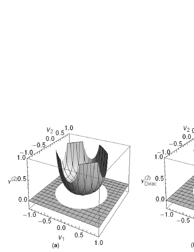
Figure 4: Comparison between (a) $\nu^{(2)}$ of the SQW⁽²⁾ and (b) $\nu^{(2)}_{\rm Dirac}$. The parameters are chosen as (a) $p=1/2,{\bf q}=(1/2,-{\rm i}/2,-1/2,{\rm i}/2)$ and (b) $\lambda/(mc)=1,{\bf q}=(1/\sqrt{2},1/\sqrt{2},0,0)$, respectively.

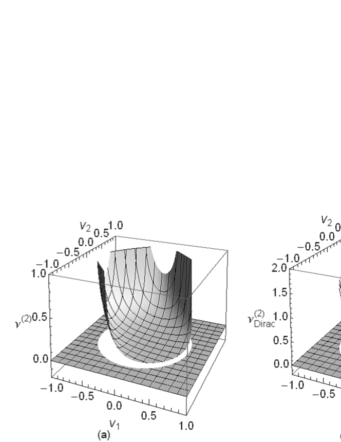
Figure 5: Comparison between (a) $\nu^{(2)}$ of the SQW⁽²⁾ and (b) $\nu^{(2)}_{\rm Dirac}$. The parameters are chosen as (a) $p=1/2,{\bf q}=(1/2,{\rm i}/2,{\rm i}/2,-1/2)$ and (b) $\lambda/(mc)=1,{\bf q}=(-(1+{\rm i})/(2\sqrt{2}),-(1+{\rm i})/(2\sqrt{2}),(1+{\rm i})/(2\sqrt{2}),(1-{\rm i})/(2\sqrt{2}))$, respectively.

III.2 One-dimensional system

By setting the momentum be a scalar $p_{1}$, we can discuss the one-dimensional system with a cutoff parameter $\lambda$. The obtained limit distribution of the one-component pseudovelocity is the following; for $\alpha_{1}\in{\bf N}_{0}$

$$\lim_{t\to\infty}\Big{\langle}V_{1}(t)^{\alpha_{1}}\Big{\rangle}_{\lambda}=\int_{-\infty}^{\infty}\frac{dv_{1}}{c}{v_{1}}^{\alpha_{1}}\nu_{\rm Dirac}^{(1)}(v_{1};\lambda,{\bf q})$$ (67)

with

$$\nu_{\rm Dirac}^{(1)}(v_{1};\lambda,{\bf q})=\mu_{\rm Dirac}^{(1)}(v_{1},\lambda){\cal M}_{\rm Dirac}^{(1)}(v_{1};{\bf q}),$$ (68)

where

$$\mu_{\rm Dirac}^{(1)}(v_{1},\lambda)=\frac{mc}{2\lambda}\frac{1}{(1-v_{1}^{2}/c^{2})^{3/2}}{\bf 1}\left(v_{1}<\sqrt{\frac{\lambda^{2}c^{2}}{(mc)^{2}+\lambda^{2}}}\right)$$ (69)

$${\cal M}_{\rm Dirac}^{(1)}(v_{1};{\bf q})=1+2v_{1}{\rm Re}(q_{1}\bar{q_{4}}+q_{2}\bar{q_{3}}).$$ (70)

The result (69) can be compared with Eq.(56) in BES07 .

Figure 6 shows the comparison between (a) $\nu^{(1)}$ of the SQW⁽¹⁾ given by (11) and (b) $\nu^{(1)}_{\rm Dirac}$ given by (68). Here we have chosen the parameters as (a) $a={\rm i}\sqrt{7/10},b={\rm i}\sqrt{3/10},{\bf q}=(1/\sqrt{2},{\rm i}/\sqrt{2})$ and (b) $\lambda/(mc)=3,{\bf q}=(1/\sqrt{2},1/\sqrt{2},0,0)$, respectively. Both distributions are symmetric. Figure 7 shows the comparison between (a) $\nu^{(1)}$ with $a=\sqrt{7/10},b={\rm i}\sqrt{3/10},{\bf q}=(1/\sqrt{5},2{\rm i}/\sqrt{5})$ and (b) $\nu^{(1)}_{\rm Dirac}$ with $\lambda/(mc)=3,{\bf q}=(1/\sqrt{10},1/\sqrt{10},2/\sqrt{10},2/\sqrt{10})$, respectively. Both show similar asymmetry.

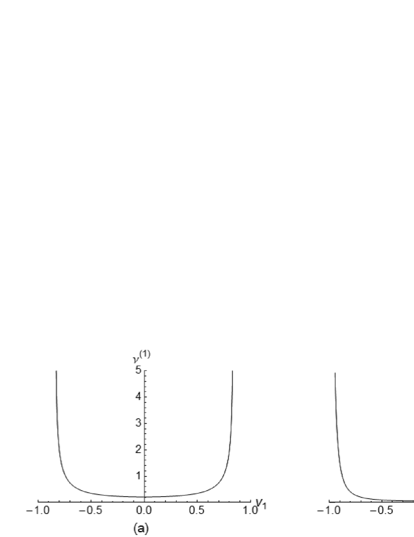
Figure 6: Comparison between (a) $\nu^{(1)}$ of the SQW⁽¹⁾ and (b) $\nu^{(1)}_{\rm Dirac}$. The parameters are chosen as (a) $a={\rm i}\sqrt{7/10},b={\rm i}\sqrt{3/10},{\bf q}=(1/\sqrt{2},{\rm i}/\sqrt{2})$ and (b) $\lambda/(mc)=3,{\bf q}=(1/\sqrt{2},1/\sqrt{2},0,0)$, respectively.

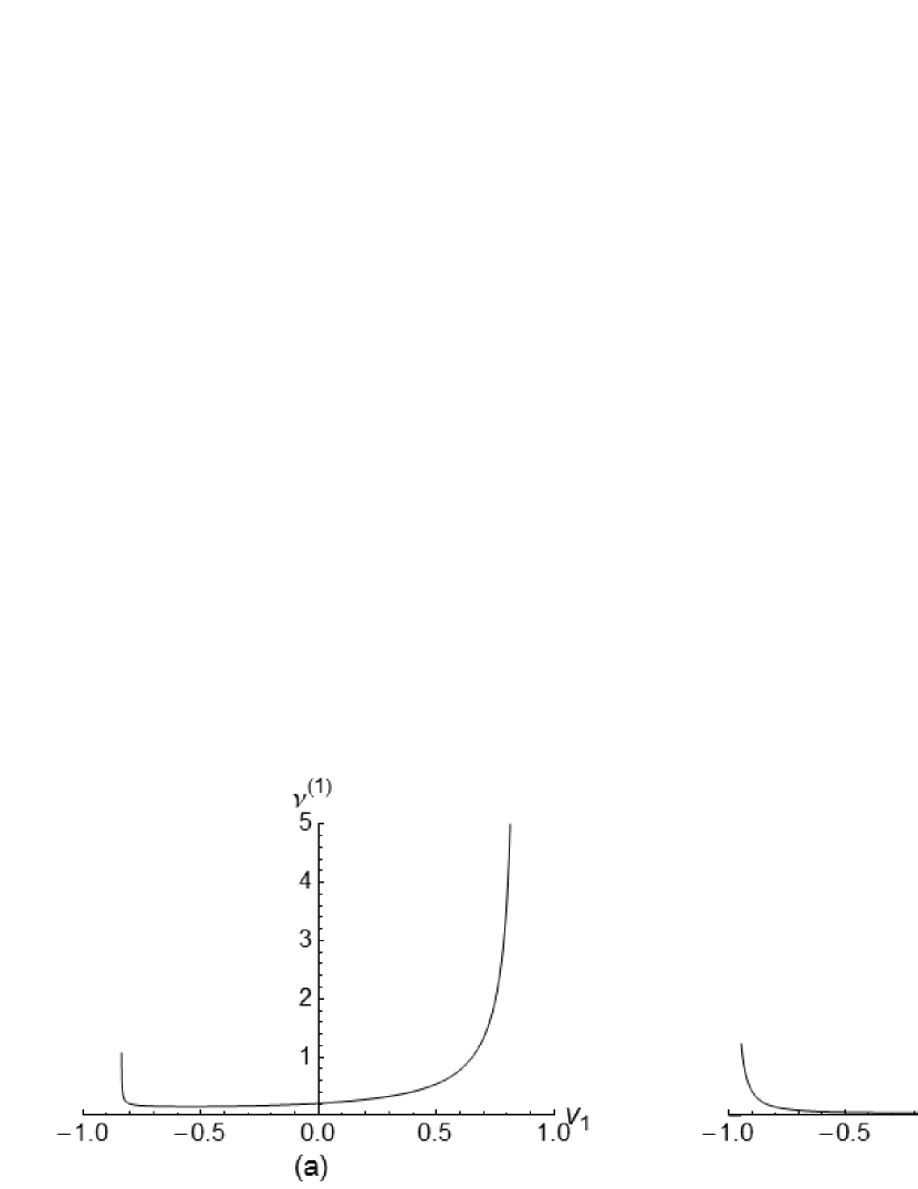
Figure 7: Comparison between (a) $\nu^{(1)}$ of the SQW⁽¹⁾ and (b) $\nu^{(1)}_{\rm Dirac}$. The parameters are chosen as (a) $a=\sqrt{7/10},b={\rm i}\sqrt{3/10},{\bf q}=(1/\sqrt{5},2{\rm i}/\sqrt{5})$ and (b) $\lambda/(mc)=3,{\bf q}=(1/\sqrt{10},1/\sqrt{10},2/\sqrt{10},2/\sqrt{10})$, respectively.

IV CONCLUDING REMARKS

In the present paper, we have shown that the novel structures of the limit distributions of pseudovelocities in the quantum walk models can be explained by the theory of relativistic quantum mechanics. We have studied a very simple system, a single free Dirac particle, but we put two special setting when we solve the Dirac equation, in order to clarify the connection with the quantum walk models. The first one is the initial condition such that the particle is located at the origin at $t=0$, and the second one is the introduction of an ultraviolet cutoff in the theory.

Importance of the study of a highly localized state of a free Dirac particle, when we consider the connection between the relativistic quantum mechanics and the quantum walk models, was clearly demonstrated by Bracken, Flohr, and Mellow BFM05 , by Strauch Str06 , and by Bracken, Ellinas, and Smyrnakis BES07 . By observing the time evolution of the wave-packet-type solutions of the Dirac equation, they found that such a highly localized initial state of a free Dirac particle leads to a rapid expansion of the distribution of position of the particle outwards from the origin, at speeds close to $c$. Our initial condition will be regarded as an ideal limit of their setting, in which the width of the wave-packet goes to zero. If we study the long-time limit of the pseudovelocity ${\bf V}(t)$ of the free Dirac particle, this phenomenon gives a singular distribution such that only on the surface of the sphere with the radius $c$ we have the delta measure, and nothing on any other points in the ${\bf V}$-space. Since the quantum walk models studied so far are defined on discrete spaces, such as lattices and trees, we have to introduce an ultraviolet cutoff in the quantum mechanics. Then the limit distributions of ${\bf V}(t)$ are moderated and we have obtained the inverted-bell shaped distribution functions. Introduction of an ultraviolet cutoff $\lambda<\infty$ in the momentum space (56) will be equivalent with the introduction of an effective size $a\propto\hbar/\lambda>0$ for the spatial initial state of a quantum particle/walker. For the one-dimensional models, systematic study of the dependence of solutions on the parameter $a$ was reported by Strauch Str07 for the discrete- and the continuous-time quantum walks and for the relativistic and non-relativistic quantum mechanics.

In the present paper, we have considered an isotropic cutoff in the momentum space by introducing a single parameter $\lambda$; $p=|{\bf p}|<\lambda$. We expect that the variety of the quantum walk models depending on lattice structure on which a quantum walker exists and choice of a quantum die represented by a unitary matrix will be partially realized by changing how to introduce cutoff in the theory. The present isotropic cutoff is too simple and thus we have some differences in symmetry of distribution functions between the graphs (a) of $\nu^{(d)}$ for the SQW^(d) and (b) of $\nu^{(d)}_{\rm Dirac}$ obtained from the Dirac equations in Figs. 4 and 5 in the $d=2$ case.

In the previous paper on the SQW⁽²⁾ WKKK08 an interesting phenomenon called the localization of quantum walker at the starting point was reported (see also IKK04 ; MKK07 ). In the present models derived from the Dirac equation, however, the localization phenomenon will not be expected.

In the present study, we have derived the limit distributions for the $d=1$ and $d=2$ systems from the result for the original Dirac equation in the three dimensions. The dependence of the results on the dimensionality $d$ will be summarized as the following,

$$\mu_{\rm Dirac}^{(d)}(v;\lambda)={\rm const.}\left(\frac{mc}{\lambda}\right)^{d}\frac{1}{(1-v^{2}/c^{2})^{(d+2)/2}}{\bf 1}\left(\frac{v}{c}<\left\{1+\left(\frac{mc}{\lambda}\right)^{2}\right\}^{-1/2}\right).$$ (71)

Note that, if we define the fifth gamma matrix by $\gamma_{5}=\gamma_{1}\gamma_{2}\gamma_{3}\gamma_{4}$ and consider the Hamiltonian operator of the form

$$\widehat{\cal H}=\gamma_{4}\left(\sum_{k=1}^{3}c\hbar\gamma_{k}\frac{\partial}{\partial x_{k}}+c\hbar\gamma_{5}\frac{\partial}{\partial x_{5}}+mc^{2}\right),$$ (72)

we can discuss the quantum walk in the four-dimensional space with the four-component qubit. Also in this case, we can obtain the limit distribution, which has the form (71) with $d=4$ as shown in Appendix A.

Appendix A Four-Dimensional System

The diagonalization of the Hamiltonian matrix corresponding to (72) can be done in the four-component momentum space ${\bf p}=(p_{1},p_{2},p_{3},p_{5})$ as follows,

$${\cal H}({\bf p})=U({\bf p})^{-1}E(p)\gamma_{4}U({\bf p})$$ (73)

with

$$U({\bf p})=\frac{1}{\sqrt{2E(p)}}\left(\sqrt{E(p)+mc^{2}}\,I_{4}+{\rm i}\sum_{k=1,2,3,5}\frac{c\gamma_{k}p_{k}}{\sqrt{E(p)+mc^{2}}}\right),$$ (74)

where $E(p)=\sqrt{(p_{1}^{2}+p_{2}^{2}+p_{3}^{2}+p_{5}^{2})c^{2}+(mc^{2})^{2}}$. Let ${\bf V}(t)=(V_{1}(t),\dots,V_{4}(t))$ be the four-component pseudovelocity. When we introduce an isotropic cutoff in the model (56), the weak limit theorem is obtained as follows; for any $\alpha_{j}\in{\bf N}_{0},1\leq j\leq 4$,

$$\lim_{t\to\infty}\left\langle\prod_{j=1}^{4}V_{j}(t)^{\alpha_{j}}\right\rangle_{\lambda}=\prod_{j=1}^{4}\int_{-\infty}^{\infty}\frac{dv_{j}}{c}\prod_{j=1}^{4}v_{j}^{\alpha_{j}}\,\nu_{\rm Dirac}^{(4)}({\bf v};\lambda,{\bf q})$$ (75)

with

$$\nu_{\rm Dirac}^{(4)}({\bf v};\lambda,{\bf q})=\mu_{\rm Dirac}^{(4)}(v;\lambda){\cal M}_{\rm Dirac}^{(4)}({\bf v};{\bf q})$$ (76)

where

$$\mu_{\rm Dirac}^{(4)}(v;\lambda)=\frac{2}{\pi^{2}}\left(\frac{mc}{\lambda}\right)^{4}\frac{1}{(1-v^{2}/c^{2})^{3}}{\bf 1}\left(v<\sqrt{\frac{\lambda^{2}c^{2}}{(mc)^{2}+\lambda^{2}}}\right),$$ (77)

$${\cal M}_{\rm Dirac}^{(4)}({\bf v};{\bf q})=1+\sum_{j=1}^{4}{\cal M}_{\rm Dirac}^{(4)}({\bf q})v_{j}$$ (78)

with

$${\cal M}_{\rm Dirac}^{(4,1)}({\bf q})=2{\rm Re}(q_{1}\bar{q_{4}}+q_{2}\bar{q_{3}}),\quad{\cal M}_{\rm Dirac}^{(4,2)}({\bf q})=2{\rm Im}(\bar{q_{1}}q_{4}-\bar{q_{2}}q_{3}),$$

$${\cal M}_{\rm Dirac}^{(4,3)}({\bf q})=2{\rm Re}(q_{1}\bar{q_{3}}-q_{2}\bar{q_{4}}),\quad{\cal M}_{\rm Dirac}^{(4,4)}({\bf q})=2{\rm Im}(\bar{q_{1}}q_{3}+\bar{q_{2}}q_{4}).$$ (79)

References

- (1) Y. Aharonov, L. Davidovich, and N. Zagury, Phys. Rev. A 48, 1687 (1993).
- (2) D. A. Meyer, J. Stat. Phys. 85, 551 (1996).
- (3) A. Nayak and A. Vishwanath, e-print quant-ph/0010117.
- (4) A. Ambainis, E. Bach, A. Nayak, A. Vishwanath, and J. Watrous, in Proc. of the 33rd Annual ACM Symp. on Theory of Computing (ACM Press, New York, 2001), pp.37-49.
- (5) B. C. Travaglione and G. J. Milburn, Phys. Rev. A 65, 032310 (2002).
- (6) N. Konno, Quantum Inf. Process 1, 345 (2002).
- (7) J. Kempe, Contemp. Phys. 44, 307 (2003).
- (8) A. Ambainis, Int. J. Quantum Inf. 1, 507 (2003).
- (9) V. M. Kendon, Int. J. Quantum Inf. 4, 791 (2006).
- (10) P. Biane, L. Bouten, F. Cipriani, N. Konno, N. Privault, Q. Xu, Quantum Potential Theory, Lecture Notes in Mathematics, 1954 (Springer, Berlin, 2008).
- (11) L. K. Grover, Phys. Rev. Lett. 79, 325 (1997).
- (12) M. A. Nielsen and I. Chuang, Quantum Computation and Quantum Information (Cambridge University Press, Cambridge, England, 2000).
- (13) A. Ambainis, in Proc. 45th Annual IEEE Symp. on Foundations of Computer Science (Piscataway, NJ, IEEE, 2004), pp.22-31.
- (14) T. Oka, N. Konno, R. Arita, and H. Aoki, Phys. Rev. Lett. 94, 100602 (2005).
- (15) M. Katori, S. Fujino, and N. Konno, Phys. Rev. A 72, 012316 (2005).
- (16) F. W. Strauch, Phys. Rev. A 73, 054302 (2006).
- (17) A. J. Bracken, D. Ellinas, and I. Smyrnakis, Phys. Rev. A 75, 022322 (2007).
- (18) F. W. Strauch, J. Math. Phys. 48, 082102 (2007).
- (19) N. Konno, J. Math. Soc. Jpn, 57, 1179 (2005).
- (20) G. Grimmett, S. Janson, and P. F. Scudo, Phys. Rev. E 69, 026119 (2004).
- (21) N. Inui, Y. Konishi, and N. Konno, Phys. Rev. A 69, 052323 (2004).
- (22) T. Miyazaki, M. Katori, and N. Konno, Phys. Rev. A 76, 012332 (2007).
- (23) K. Watabe, N. Kobayashi, M. Katori, and N. Konno, Phys. Rev. A 77, 062331 (2008).
- (24) E. Segawa and N. Konno, Int. J. of Quantum Inf., 6, 1231 (2008).
- (25) N. Konno, Quantum Inf. Process 8, 387 (2009).
- (26) J. D. Bjorken and S. D. Drell, Relativistic Quantum Mechanics (McGraw-Hill, New York, 1964).
- (27) P. A. M. Dirac, The Principles of Quantum Mechanics, 4th edn (Clarendon Press, Oxford, 1958).
- (28) C. Itzykson and J-B. Zuber, Quantum Field Theory (McGraw-Hill, New York, 1980).
- (29) A. J. Bracken, J. A. Flohr, and G. F. Melloy, Proc. R. Soc. A 461, 3633 (2005).
- (30) L. L. Foldy and A. Wouthuysen, Phys. Rev. 78, 29 (1950).
- (31) S. Tani, Prog. Theor. Phys. 6, 267 (1951).