Scaling limit of the invasion percolation cluster on a regular tree

Abstract

We prove existence of the scaling limit of the invasion percolation cluster (IPC) on a regular tree. The limit is a random real tree with a single end. The contour and height functions of the limit are described as certain diffusive stochastic processes.

This convergence allows us to recover and make precise certain asymptotic results for the IPC. In particular, we relate the limit of the rescaled level sets of the IPC to the local time of the scaled height function.

, and

OAmarkSupported in part by NSERC.

MMmarkSupported in part by the Pacific Institute for the Mathematical Sciences.

1 Introduction and main results

Invasion percolation on an infinite connected graph is a random growth model which is closely related to critical percolation, and is a prime example of self-organized criticality. It was introduced in the eighties by Wilkinson and Willemsen WilkWillem1983 and first studied on the regular tree by Nickel and Wilkinson NickWilk1983 . The relation between invasion percolation and critical percolation has been studied by many authors (see, e.g., CCN1985 , Jarai2003 ). More recently, Angel, Goodman, den Hollander and Slade AGdHS2008 have given a structural representation of the invasion percolation cluster on a regular tree, and used it to compute the scaling limits of various quantities related to the IPC such as the distribution of the number of invaded vertices at a given level of the tree.

Fixing a degree $\sigma\geq 2$, we consider ${\mathcal{T}}={\mathcal{T}}_{\sigma}$: the rooted regular tree with index $\sigma$, that is, the rooted tree where every vertex has $\sigma$ children. Invasion percolation on ${\mathcal{T}}$ is defined as follows: edges of ${\mathcal{T}}$ are assigned weights which are i.i.d. and uniform on $[0,1]$. The invasion percolation cluster on ${\mathcal{T}}$, denoted IPC, is grown inductively starting from a subgraph $I_{0}$ consisting of the root $\varnothing$ of ${\mathcal{T}}$. At each step $I_{n+1}$ consists of $I_{n}$ together with the edge of minimal weight in the boundary of $I_{n}$. The invasion percolation cluster IPC is the limit $\bigcup I_{n}$.

1.1 Convergence of trees

We consider the IPC as a metric space with respect to graph distance $d_{\mathrm{gr}}$. Since IPC is already infinite, taking its scaling limit amounts to replacing $d_{\mathrm{gr}}$ by $\frac{1}{k}d_{\mathrm{gr}}$.

Theorem 1.1

The rescaled rooted invasion percolation cluster $(\mbox{IPC},\break\frac{1}{k}d_{\mathrm{gr}}$, $\varnothing)$ has a scaling limit w.r.t. the pointed Gromov–Hausdorff topology, which is a random ${\mathbb{R}}$-tree.

Here, an ${\mathbb{R}}$-tree means a topological space with a unique rectifiable simple path between any two points. Note that, because the IPC is infinite, we must work with the pointed Gromov–Hausdorff topology (see, e.g., Munn2010 , Section 2). For present purposes this means we must show that, for each $R>0$, the ball $\{v\in\mathrm{IPC}\dvtx\frac{1}{k}d_{\mathrm{gr}}(\varnothing,x)\leq R\}$ about the root converges in the Gromov–Hausdorff sense.

A key point in our study is that the contour function (as well as height function and Lukaciewicz path, see Section 5.4 below) of an infinite tree does not generally encode the entire tree. If the various encodings of trees are applied to infinite trees, they describe only the part of the tree to the left of the leftmost infinite branch. We present two ways to overcome this difficulty. Both are based on the fact (see AGdHS2008 ) that the IPC has a.s. a unique infinite branch. Following Aldous Aldous1991 , we define a sin-tree to be an infinite one-ended tree (i.e., with a single infinite branch).

The first approach is to use the symmetry of the underlying graph ${\mathcal{T}}$ and observe that the infinite branch of the IPC (called the backbone) is independent of the metric structure of the IPC. Thus, for all purposes involving only the metric structure of the IPC, we may as well assume (or condition) that the backbone is the rightmost branch of ${\mathcal{T}}$. We denote by ${\mathcal{R}}$ the IPC under this condition. The various encodings of ${\mathcal{R}}$ encode the entire tree.

The second approach is to consider a pair of encodings, one for the part of the tree to the left of the backbone, and a second encoding the part to the right of the backbone. This is done by considering also the encoding of the reflected tree $\overline{\mbox{IPC}}$. The reflection of a plane tree is defined to be the same tree with the reversed order for the children of each vertex. The uniqueness of the backbone implies that together the two encodings determine the entire IPC.

In order to describe the limits, we first define the process $L(t)$ which is the lower envelope of a Poisson process on $({\mathbb{R}}^{+})^{2}$. Given a Poisson process ${\mathcal{P}}$ of intensity 1 in the quarter plane, $L(t)$ is defined by

$$L(t)=\inf\{y\dvtx(x,y)\in{\mathcal{P}}\mbox{ and }x\leq t\}.$$

Our other results describe the scaling limits of the various encodings of the trees in terms of solutions of

$$Y_{t}=B_{t}-\int_{0}^{t}L(-\underline{Y}_{s})\,ds, {\mathcal{E}}(L)$$ ()

where $\underline{Y}_{s}=\inf_{0\leq u\leq s}Y_{u}$ is the infimum process of $Y$ and $B_{t}$ is a standard Brownian motion. The reason for the notation is that we also consider solutions of equations ${\mathcal{E}}(L/2)$ where, in the above, $L$ is replaced by $L/2$. Note that by the scale invariance of the Poisson process, $kL(kt)$ has the same law as $L(t)$. Hence, the scaling of Brownian motion implies that the solution $Y$ has Brownian scaling as well.

We work primarily in the space ${\mathcal{C}}({\mathbb{R}}^{+},{\mathbb{R}}^{+})$ of continuous functions from ${\mathbb{R}}^{+}$ to itself with the topology of locally uniform convergence. We consider three well known and closely related encodings of plane trees, namely, the Lukaciewicz path, and the contour and height functions (all are defined in Section 2.3 below). The three are closely related and, indeed, their scaling limits are almost the same. The reason for the triplication is that the contour function is the simplest and most direct encoding of a plane tree, whereas the Lukaciewicz path turns out to be easier to deal with in practice. The height function is a middle ground.

Theorem 1.2

For the IPC conditioned on the backbone being on the right, let $V_{\mathcal{R}}$, $H_{\mathcal{R}}$ and $C_{\mathcal{R}}$ denote its Lukaciewicz path, height function and contour function, respectively. Then we have the following weak limits in ${\mathcal{C}}({\mathbb{R}}^{+},{\mathbb{R}})$:

$$(k^{-1}V_{\mathcal{R}}(k^{2}t))_{t\geq 0} \to \bigl{(}\gamma^{1/2}(Y_{t}-\underline{Y}_{t})\bigr{)}_{t\geq 0},$$ (1)

$$(k^{-1}H_{\mathcal{R}}(k^{2}t))_{t\geq 0} \to \bigl{(}\gamma^{-1/2}(2Y_{t}-3\underline{Y}_{t})\bigr{)}_{t\geq 0},$$ (2)

$$(k^{-1}C_{\mathcal{R}}(2k^{2}t))_{t\geq 0} \to \bigl{(}\gamma^{-1/2}(2Y_{t}-3\underline{Y}_{t})\bigr{)}_{t\geq 0}$$ (3)

as $k\to\infty$, where

$$\gamma=\frac{\sigma-1}{\sigma}$$

and $(Y_{t})_{t\geq 0}$ is the solution of (${\mathcal{E}}(L)$) (and is the same solution in all three limits).

To put this theorem into context, recall that the Lukaciewicz path of a critical Galton–Watson tree is an excursion of random walk with i.i.d. steps. From this it follows that the path of an infinite sequence of critical trees scales to Brownian motion. The height and contour functions of the sequence are easily expressed in terms of the Lukaciewicz path and, assuming the branching law has second moments, are seen to scale to reflected Brownian motion (cf. Le Gall LeGall2005 ). Duquesne and Le Gall generalized this approach in DuqLeG2002 , and showed that the genealogical structure of a continuous-state branching process is similarly coded by a height process which can be expressed in terms of a Lévy process, and that this is also the limit of various Galton–Watson trees with heavy tails.

The case of sin-trees is considered by Duquesne Duquesne2005 to study the scaling limit of the range of a random walk on a regular tree. His techniques suffice for analysis of the IIC, but the IPC requires additional ideas, the key difficulty being that the Lukaciewicz path is no longer a Markov process. The scaling limit of the IIC turns out to be an illustrative special case of our results, and we will describe its scaling limit as well (in Section 4.6).

For the unconditioned IPC we define its left part $\mbox{IPC}_{G}$ to be the subtree consisting of the backbone and all vertices to its left. The right part $\mbox{IPC}_{D}$ is defined as the left part of the reflected IPC. We can now define $V_{G}$ and $V_{D}$ to be, respectively, the Lukaciewicz paths for the left and right parts of the IPC, and similarly define $H_{G},H_{D},C_{G},C_{D}$ (see also Section 2.4 below).

Theorem 1.3

We have the following weak limits in ${\mathcal{C}}({\mathbb{R}}^{+},{\mathbb{R}})$:

$$k^{-1}(V_{G}(k^{2}t),V_{D}(k^{2}t))_{t\geq 0} \to \gamma^{1/2}(Y_{t}-\underline{Y}_{t},\widetilde{Y}_{t}-\underline{\widetilde{Y}}_{t})_{t\geq 0},$$ (4)

$$k^{-1}(H_{G}(k^{2}t),H_{D}(k^{2}t))_{t\geq 0} \to \gamma^{-1/2}(Y_{t}-2\underline{Y}_{t},\widetilde{Y}_{t}-2\underline{\widetilde{Y}}_{t})_{t\geq 0},$$ (5)

$$k^{-1}(C_{G}(2k^{2}t),C_{D}(2k^{2}t))_{t\geq 0} \to \gamma^{-1/2}(Y_{t}-2\underline{Y}_{t},\widetilde{Y}_{t}-2\underline{\widetilde{Y}}_{t})_{t\geq 0}$$ (6)

as $k\to\infty$, where $(Y_{t})_{t\geq 0}$ and $(\widetilde{Y}_{t})_{t\geq 0}$ are independent solutions of ${\mathcal{E}}(L/2)$.

1.2 Level sizes and volumes

From the convergence results above we can establish asymptotics for level sizes and volumes in the invasion percolation cluster. In AGdHS2008 , it was proved that the size of the $n$th level of the IPC, rescaled by a factor $n$, converges to a nondegenerate limit. Similarly, the volume up to level $n$, rescaled by a factor $n^{2}$, converges to a nondegenerate limit. The Laplace transforms of these limits were expressed as functions of the $L$-process. However, formulas (1.20)–(1.23) of AGdHS2008 do not provide insight into the limiting variables. With our convergence theorem for height functions of ${\mathcal{R}}$, we can express the limit in terms of the continuous limiting height function.

For $x\in{\mathbb{R}}_{+}$ we denote by $C[x]$ the number of vertices of the IPC at height $[x]$. We let $C[0,x]=\sum_{i=0}^{[x]}C[i]$ denote the number of vertices of the IPC up to height $[x]$. Write $H_{t}=\gamma^{-1/2}(2Y_{t}-3\underline{Y}_{t})$ for the limit of $H_{\mathcal{R}}$ in Theorem 1.2, and $l_{\infty}^{a}(H)$ for the standard local time at level $a$ of $H$.

Theorem 1.4

For every $a>0$ we have the distributional limits

$$\frac{1}{n^{2}}C[0,an]\displaystyle\mathop{\hbox to28.45274pt{\rightarrowfill}}_{n\to\infty}\int_{0}^{\infty}\mathbf{1}_{[0,a]}(H_{s})\,ds$$ (7)

and

$$\frac{1}{n}C[an]\displaystyle\mathop{\hbox to28.45274pt{\rightarrowfill}}_{n\to\infty}\frac{\gamma}{4}l_{\infty}^{a}(H).$$ (8)

In the case of the asymptotics of the levels, we also provide an alternative way of expressing the limit directly as a sum of independent variables. Write $\mathbf{e}\{c\}$ for an exponential variable of rate $c$.

Theorem 1.5

Let $S$ be a point process such that, conditioned on the $L$-process, $S$ is an inhomogeneous Poisson point process on $[0,a\sqrt{\gamma}]$, with intensity

$$\frac{2L(s)\,ds}{\exp((a\sqrt{\gamma}-s)L(s))-1}.$$

Then, conditionally on $L$, and in distribution,

$$\frac{1}{n}C[an]\displaystyle\mathop{\hbox to28.45274pt{\rightarrowfill}}_{n\to\infty}\frac{\sqrt{\gamma}}{2}\sum_{s\in S}\mathbf{e}\biggl{\{}\frac{L(s)}{1-\exp(-(a\sqrt{\gamma}-s)L(s))}\biggr{\}},$$ (9)

where the terms in the sum are independent.

From this representation and properties of the $L$-process, it is straightforward to recover the representation of the asymptotic Laplace transform of level sizes, (1.21) of AGdHS2008 . Also, as the proof of the theorem will show, a.s. only a finite number of distinct values of $L$ contribute to the sum in (9).

1.3 Application to the incipient infinite cluster

The proofs of Theorems 1.1–1.5 also apply to the incipient infinite cluster (IIC), whose structure and similarity to the IPC we outline in Section 2.2. Stated briefly, the IIC corresponds to the IPC in the simpler case where the process $L(t)$ is replaced by $0$. As a consequence, some elements of the proofs (such as the right-grafting constructions in Section 5) are not needed to handle the IIC. For comparison, we summarize the results for the IIC in the following theorems.

Theorem 1.6

The rescaled rooted incipient infinite cluster $(\mbox{IIC},\frac{1}{k}d_{\mathrm{gr}},\varnothing)$ has a scaling limit w.r.t. the pointed Gromov–Hausdorff topology, which is a random ${\mathbb{R}}$-tree.

For the IIC conditioned on the backbone being on the right, let $V_{\mathcal{R}}^{\mathrm{IIC}}$, $H_{\mathcal{R}}^{\mathrm{IIC}}$ and $C_{\mathcal{R}}^{\mathrm{IIC}}$ denote its Lukaciewicz path, height function and contour function, respectively. Then we have the following weak limits in ${\mathcal{C}}({\mathbb{R}}^{+},{\mathbb{R}})$:

$$(k^{-1}V_{\mathcal{R}}^{\mathrm{IIC}}(k^{2}t))_{t\geq 0} \to \bigl{(}\gamma^{1/2}(B_{t}-\underline{B}_{t})\bigr{)}_{t\geq 0},$$ (10)

$$(k^{-1}H_{\mathcal{R}}^{\mathrm{IIC}}(k^{2}t))_{t\geq 0} \to \bigl{(}\gamma^{-1/2}(2B_{t}-3\underline{B}_{t})\bigr{)}_{t\geq 0},$$ (11)

$$(k^{-1}C_{\mathcal{R}}^{\mathrm{IIC}}(2k^{2}t))_{t\geq 0} \to \bigl{(}\gamma^{-1/2}(2B_{t}-3\underline{B}_{t})\bigr{)}_{t\geq 0}$$ (12)

as $k\to\infty$, where $B_{t}$ is a standard Brownian motion.

For the IIC with unconditioned backbone, the Lukaciewicz paths, height functions and contour functions of its left and right parts have the following weak limits in ${\mathcal{C}}({\mathbb{R}}^{+},{\mathbb{R}})$:

$$k^{-1}(V_{G}^{\mathrm{IIC}}(k^{2}t),V_{D}^{\mathrm{IIC}}(k^{2}t))_{t\geq 0} \to \gamma^{1/2}(B_{t}-\underline{B}_{t},\widetilde{B}_{t}-\underline{\widetilde{B}}_{t})_{t\geq 0},$$ (13)

$$k^{-1}(H_{G}^{\mathrm{IIC}}(k^{2}t),H_{D}^{\mathrm{IIC}}(k^{2}t))_{t\geq 0} \to \gamma^{-1/2}(B_{t}-2\underline{B}_{t},\widetilde{B}_{t}-2\underline{\widetilde{B}}_{t})_{t\geq 0},$$ (14)

$$k^{-1}(C_{G}^{\mathrm{IIC}}(2k^{2}t),C_{D}^{\mathrm{IIC}}(2k^{2}t))_{t\geq 0} \to \gamma^{-1/2}(B_{t}-2\underline{B}_{t},\widetilde{B}_{t}-2\underline{\widetilde{B}}_{t})_{t\geq 0}$$ (15)

as $k\to\infty$, where $B_{t}$ and $\widetilde{B}_{t}$ are independent Brownian motions.

Note that up to constant factors, the scaling limits in (10) and (13) are reflected Brownian motions, while the scaling limits in (14) and (15) are three-dimensional Bessel processes. The scaling limit in (11) and (12), however, is not a standard process.

Theorem 1.7

Write $H_{t}^{\mathrm{IIC}}=\gamma^{-1/2}(2Y_{t}-3\underline{Y}_{t})$ for the limit of $H_{\mathcal{R}}^{\mathrm{IIC}}$ in (11), and $l_{\infty}^{a}(H)$ for the standard local time at level $a$ of $H$. Then for every $a>0$ we have the distributional limits

$$\frac{1}{n^{2}}C[0,an]\displaystyle\mathop{\hbox to28.45274pt{\rightarrowfill}}_{n\to\infty}\int_{0}^{\infty}\mathbf{1}_{[0,a]}(H_{s})\,ds$$ (16)

and

$$\frac{1}{n}C[an]\displaystyle\mathop{\hbox to28.45274pt{\rightarrowfill}}_{n\to\infty}\frac{\gamma}{4}l_{\infty}^{a}(H).$$ (17)

Moreover, if $S^{\mathrm{IIC}}$ is an inhomogeneous Poisson point process on $[0,a\sqrt{\gamma}]$ with intensity $2(a\sqrt{\gamma}-s)^{-1}\,ds$, then

$$\frac{1}{n}C[an]\displaystyle\mathop{\hbox to28.45274pt{\rightarrowfill}}_{n\to\infty}\frac{\sqrt{\gamma}}{2}\sum_{s\in S}\mathbf{e}\bigl{\{}\bigl{(}a\sqrt{\gamma}-s\bigr{)}^{-1}\bigr{\}}$$ (18)

in distribution, where the terms in the sum are independent.

2 Background and overview

2.1 Structure of the IPC

We now give a brief overview of the IPC structure theorem from AGdHS2008 , which is the basis for the present work. First of all, the IPC contains a single infinite branch, called the backbone and denoted BB. The backbone is a uniformly random branch in the tree (in the natural sense). From the backbone emerge, at every height $n$ and on every edge away from the backbone, subcritical percolation clusters with parameter $\widehat{W}_{n}<p_{c}=\sigma^{-1}$.

The parameters $\widehat{W}_{n}$ are nondecreasing and satisfy $\widehat{W}_{n}\displaystyle\mathop{\hbox to28.45274pt{\rightarrowfill}}_{n\to\infty}p_{c}$. Moreover, $(\widehat{W}_{n})_{n=0}^{\infty}$ forms a Markov chain with dynamics of the following kind. The initial value $\widehat{W}_{0}$ is distributed on $[0,p_{c}]$ according to a certain density function $f$. Given $\widehat{W}_{n}=\widehat{w}$, the next value $\widehat{W}_{n+1}$ is, with probability $g(\widehat{w})$, a new value chosen according to the density $f$ conditioned to be larger than $\widehat{w}$; or else, with probability $g(\widehat{W}_{n})$, the value $\widehat{w}$. For our purposes, it will suffice to know that the functions $f$ and $g$ satisfy

$$\lim_{\widehat{w}\nearrow p_{c}}f(\widehat{w})>0,\qquad g(\widehat{w})\sim\sigma(p_{c}-\widehat{w})=1-\sigma\widehat{w}$$ (19)

as $\widehat{w}\nearrow p_{c}$. (These asymptotics follow from AGdHS2008 , Sections 2.1.2 and 3.1, since $(\widehat{W}_{n})_{n=0}^{\infty}$ is the image of the Markov chain $(W_{n})_{n=0}^{\infty}$ under $w\mapsto\widehat{w}$.)

We will primarily be concerned with the scaling limit of $\widehat{W}_{n}$, which is given by the lower envelope process $L(t)$ defined above. Writing $[x]$ for the integer part of $x$, we have, for any $\varepsilon>0$,

$$\bigl{(}k\bigl{(}1-\sigma\widehat{W}_{[kt]}\bigr{)}\bigr{)}_{t\geq\varepsilon}\displaystyle\mathop{\hbox to28.45274pt{\rightarrowfill}}_{k\to\infty}(L(t))_{t\geq\varepsilon}$$ (20)

with respect to the Skorohod topology (see AGdHS2008 , Proposition 3.3 and Corollary 3.4). Indeed, $L(t)$ is the continuous-time process that jumps, at rate $L(t)$, to a value uniformly chosen between $0$ and $L(t)$; this reflects the asymptotics given in (19).

The process $L_{t}$ diverges as $t\to 0$, which somewhat complicates the study of the IPC close to the root.

2.2 Structure of the IIC

The incipient infinite cluster (IIC) embodies the notion of a percolation cluster that is both critical and infinite. It was originally defined and discussed by Kesten Kesten1986 (see also BarKum2006 ). The IIC can be obtained through a variety of limiting constructions—for instance, by conditioning a critical percolation cluster to extend at least distance $R$ and sending $R\to\infty$, or by examining the neighborhood of a faraway point in the IPC (see Jarai2003 and AGdHS2008 , Theorem 1.2). In the present context, we note that the IIC on a regular tree has a structure similar to the IPC; see AGdHS2008 , Section 2.1.

Specifically, the IIC contains a single infinite branch, the backbone, which is a uniformly random branch in the tree. From the backbone emerge, at every height and on every edge away from the backbone, critical percolation clusters.

Note that setting $\widehat{W}_{n}\equiv p_{c}$ in the above description gives rise to the IIC, on the one hand, while in the scaling limit $L$ is replaced by 0. This enables us to use a common framework for both clusters.

The convergence $\widehat{W}_{n}\displaystyle\mathop{\hbox to28.45274pt{\rightarrowfill}}_{n\to\infty}p_{c}$ explains why the IPC and IIC resemble each other far above the root. However, the analysis of AGdHS2008 shows that the convergence of the parameter of the attached clusters is slow enough that $r$-point functions and other measurable quantities such as level sizes possess different scaling limits.

2.3 Encodings of finite trees

For completeness we include here the definition of the various tree encodings we are concerned with. We refer to Le Gall LeGall2005 for further details in the case of finite trees and to Duquesne Duquesne2005 in the case of sin-trees discussed below.

A rooted plane tree $\theta$ (also called an ordered tree) is a tree with a description as follows. Vertices of $\theta$ belong to $\bigcup_{n\geq 0}{\mathbb{N}}^{n}$. By convention, $\varnothing\in{\mathbb{N}}^{0}$ is always a vertex of $\theta$ which is called the root. For a vertex $v\in\theta$, we let $k_{v}=k_{v}(\theta)$ be the number of children of $v$ and whenever $k_{v}=k>0$, these children are denoted $v1,\ldots,vk$. In particular, the $i$th child of the root is simply $i$, and if $vi\in\theta$, then $\forall 1\leq j<i$, $vj\in\theta$ as well. Edges of $\theta$ are the edges $(v,vi)$ whenever $vi\in\theta$. Note that the set of edges of $\theta$ are determined by the set of vertices and vice-versa, which allows us to blur the distinction between a tree and its set of vertices. The $k$th generation of a tree contains every vertex $v\in\theta\cap{\mathbb{N}}^{k}$, so that the $0$th generation consists exactly of the root. Define $\#\theta$ to be the total number of vertices in $\theta$.

Let $(v^{i})_{0\leq i<\#\theta}$ be the vertices of $\theta$ listed in lexicographic order, so that $v^{0}=\varnothing$. The Lukaciewicz path $V$ of $\theta$ (sometimes known as the depth-first path) is the continuous function $(V_{t}=V^{\theta}_{t},t\in[0,\#\theta])$ defined as follows: for $n\in\{1,\ldots,\#\theta\}$

$$V_{n}=V^{\theta}_{n}:=\sum_{i=0}^{n-1}(k_{v^{i}}-1),$$

and between integers $V$ is interpolated linearly.

The values $V_{n}$ are also given by the following right-hand description of the Lukaciewicz path. This description is simpler to visualize, though we do not know of a reference for it. For $v\in\theta$, consider the subtree $\theta^{v}\subset\theta$ formed by all the vertices which are smaller or equal to $v$ in the lexicographic order. Let $n(v,\theta)$ be the number of edges connecting vertices of $\theta^{v}$ with vertices of $\theta\setminus\theta^{v}$. Then

$$V(k)=n(v^{k},\theta)-1.$$

The reason we call this the right-hand description is that $n(v,\theta)$ is also the number of edges attached on the right-hand side of the path from $\varnothing$ to $v$. It is straightforward to check that this description is consistent with other definitions.

The height function is the second encoding we wish to consider. We also define it to be a piecewise linear function with $H(k)$ the height of $v^{k}$ above the root. It is related to the Lukaciewicz path by

$$H(n)=\#\bigl{\{}k<n\dvtx V_{k}=\min\{V_{k},\ldots,V_{n}\}\bigr{\}}.$$ (21)

Finally, the contour function of $\theta$ is obtained by considering a walker exploring $\theta$ at constant unit speed, starting from the root at time 0, and going from left to right. Each edge is traversed twice (once on each side), so that the total time before returning to the root is $2(\#\theta-1)$. The value $C^{\theta}(t)$ of the contour function at time $t\in[0,2(\#\theta-1)]$ is the distance between the walker and the root at time $t$.

It is straightforward to check that the Lukaciewicz path, height function and contour function each uniquely determine—and hence represent—any finite tree $\theta$. Figure 1 illustrates these definitions, as they are easier to understand from a picture.

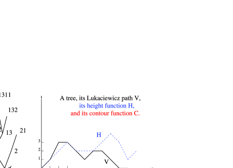
Figure 1: A finite tree and its encodings.

At times it is useful to encode a sequence of finite trees by a single function. This is done by concatenating the Lukaciewicz paths or height function of the trees of the sequence. Note that when coding a sequence of trees, jumping from one tree to the next corresponds to reaching a new integer infimum in the Lukaciewicz path, while it corresponds to a visit to 0 in the height process.

2.4 Encoding sin-trees

While the definitions of Lukaciewicz path, and height and contour functions, extend immediately to infinite (discrete) trees, these paths generally no longer encode a unique infinite tree. For example, all the trees containing the infinite branch $\{\varnothing,1,11,111,\ldots\}$ would have the identity function for height function, so that equal paths correspond to distinct infinite trees. In fact, the only part of an infinite tree which one can recover from the the height and contour functions is the subtree that lies left of the leftmost infinite branch. The Lukaciewicz path encodes additionally the degrees of vertices along the leftmost infinite branch.

However, if we restrict the encodings to the class of trees whose only infinite branch is the rightmost branch, then the three encodings still correspond to unique trees. In particular, observe that $\mbox{IPC}_{G}$ and ${\mathcal{R}}$ are fully encoded by their Lukaciewicz paths (as well as by their height, or contour functions). That is the reason we begin our discussion with these conditioned objects.

Not surprisingly, it is possible to encode any sin-tree, such as the IIC and IPC, by using two coding paths, one for the part of the tree lying to the left of the backbone, and one for the part lying to its right. More precisely, suppose ${\mathcal{T}}$ is a sin-tree, and BB denotes its backbone. The left tree is defined as the set of all vertices on or to the left of the backbone:

$${\mathcal{T}}_{G}:=\bigcup_{v\in\mathrm{BB}}{\mathcal{T}}^{v}=\{x\in{\mathcal{T}}\dvtx\exists v\in\mbox{BB},x\leq v\}.$$

We do not define the right-tree of ${\mathcal{T}}$ as the set of vertices which lie on or to the right of the backbone. Rather, in light of the way the encodings are defined, it is easier to work with the mirror-image of ${\mathcal{T}}$, denoted $\overline{{\mathcal{T}}}$ and defined as follows: since a plane tree is a tree where the children of each vertex are ordered, $\overline{{\mathcal{T}}}$ may be defined as the same tree but with the reverse order on the children at each vertex. We then define

$${\mathcal{T}}_{D}=(\overline{{\mathcal{T}}})_{G}.$$

Obviously, only the rightmost branches of ${\mathcal{T}}_{G},{\mathcal{T}}_{D}$ are infinite, so the Lukaciewicz paths $V_{G},V_{D}$, of ${\mathcal{T}}_{G},{\mathcal{T}}_{D}$, do encode uniquely each of these two trees (and so do the height functions $H_{G},H_{D}$ and the contour functions $C_{G},C_{G}$). Therefore, the pair of paths $(V_{G},V_{D})$ encodes ${\mathcal{T}}$ [and so do the pairs $(H_{G},H_{D})$, $(C_{G},C_{D})$]. Note that $H_{G},C_{G}$ are also, respectively, the height and contour functions of ${\mathcal{T}}$ itself, while $H_{D},C_{D}$ are, respectively, the height and contour functions of $\overline{{\mathcal{T}}}$.

2.5 Overview

Let us try to give briefly, and heuristically, some intuition of why Theorem 1.2 holds. For $t>0$, the tree emerging from $\mbox{BB}_{[kt]}$ is coded by the $[kt]$th excursion of $V$ above $0$. Except for its first step, this excursion has the same transition probabilities as a random walk with drift $\sigma\widehat{W}_{[kt]}-1$, which, by the convergence (20), is approximately $-L(t)/k$. Additionally, by AGdHS2008 , Proposition 3.1, $\widehat{W}_{n}$ is constant for long stretches of time. It is well known (see, e.g., Jacod1985 , Theorem 2.2.1) that a sequence of random walks with drift $c/k$, suitably scaled, converges as $k\to\infty$ to a $c$-drifted Brownian motion. Thus, we expect to find segments of drifted Brownian paths in our limit. According to the convergence (20), the drift is expressed in terms of the $L$-process. This is what the definition of $Y$ expresses.

Thus, the idea when dealing with either the conditioned or the unconditioned IPC is to cut these sin-trees into pieces corresponding to stretches where $\widehat{W}$ is constant, and to look separately at the convergence of each piece. Since we deal extensively with codings of trees by paths, we call these pieces of trees segments, although in the terminology of NewmanStein1995 , GoodmanPondsInPrep , DamronSapozhnikov2010 and other works they are known as the ponds of the IPC.

In Section 3 we establish existence and uniqueness results for equation (${\mathcal{E}}(L)$).

In Section 4 we look at the convergence of the rescaled paths coding a sequence of such segments for well chosen, fixed values of the $\widehat{W}$-process. In fact, we consider slightly more general settings which allows us to treat the case of the IIC as well as the various flavors of the IPC.

In Section 5 we prove Theorem 1.2 and Theorem 1.3 by combining segments. To deal with the fact that $\widehat{W}$ is random and exploit the convergence (20), we use a coupling argument (see Section 5.2). We then prove that the segments fall into the family dealt with in Section 4. Because of the divergence of the $L$-process at the origin, we only perform the above for subtrees above certain levels, and bound the resulting error separately. The proof of Theorem 1.1 follows from Theorem 1.2.

Finally, in Section 6 we apply our convergence results to establish asymptotics for level and volume estimates of the IPC, to recover and extend results of AGdHS2008 .

3 Solving (${\mathcal{E}}(L)$)

Claim 3.1

Solutions to (${\mathcal{E}}(L)$), ${\mathcal{E}}(L/2)$ are unique in law.

Curiously, we were unable to determine whether the solutions to (${\mathcal{E}}(L)$) are a.s. pathwise unique (i.e., whether strong uniqueness holds). For our purposes uniqueness in law suffices. Proof of Claim 3.1 We prove this claim for equation (${\mathcal{E}}(L)$). The proof for equation ${\mathcal{E}}(L/2)$ is identical.

Let $Y$ be a solution of (${\mathcal{E}}(L)$). Since $L$ is positive, $Y_{t}\leq B_{t}$. Since $L$ is nonincreasing, $\int_{0}^{t}L(-\underline{Y}_{s})\,ds\leq\int_{0}^{t}L(-\underline{B}_{s})\,ds$. For any fixed $\varepsilon>0$, a.s. for all small enough $s$, $-\underline{B}_{s}>s^{1/2-\varepsilon}$, while a.s. for all small enough $u$, $L(u)<u^{-(1+\varepsilon)}$. We deduce that almost surely $\lim_{t\to 0}\int_{0}^{t}L(-\underline{Y}_{s})\,ds=0$. Thus, any solution of (${\mathcal{E}}(L)$) is continuous.

Let us now consider two solutions $Y^{1}$, $Y^{2}$ of $\mathcal{E}(L)$ and fix $\varepsilon>0$. Introduce

$$j^{\varepsilon}:=\inf\{t>0\dvtx L(t)<\varepsilon^{-1}\}$$

and

$$t_{0}^{\varepsilon} := \inf\{t>0\dvtx-\underline{B}_{t}>j^{\varepsilon}\},$$

$$t_{1}^{\varepsilon} := \inf\{t>0\dvtx-\underline{Y}^{1}_{t}>j^{\varepsilon}\},$$

$$t_{2}^{\varepsilon} := \inf\{t>0\dvtx-\underline{Y}^{2}_{t}>j^{\varepsilon}\}.$$

From the continuity of $Y^{1},Y^{2}$ we have $Y^{1}(t_{1}^{\varepsilon})=Y^{2}(t_{2}^{\varepsilon})=-j^{\varepsilon}$. Moreover, we have a.s. $t_{1}^{\varepsilon}\vee t_{2}^{\varepsilon}\leq t_{0}^{\varepsilon}$, and, therefore,

$$t_{1}^{\varepsilon}\vee t_{2}^{\varepsilon}\displaystyle\mathop{\hbox to28.45274pt{\rightarrowfill}}_{\varepsilon\to 0}^{\mathrm{a.s.}}0.$$ (22)

Introduce a Brownian motion $\beta$ independent of $B$ and consider the (SDE)

$$Z_{t}^{\varepsilon}=\beta_{t}-\int_{0}^{t}L(j^{\varepsilon}-\underline{Z}^{\varepsilon}_{s})\,ds. {\mathcal{E}}(\varepsilon,L)$$ ()

Pathwise existence and uniqueness hold for (${\mathcal{E}}(\varepsilon,L)$) by standard arguments.

We then define

$$Y^{1,\varepsilon}_{t} = \cases{Y^{1}_{t},&\quad if $t<t_{1}^{\varepsilon}$,\cr Y^{1}_{t_{1}^{\varepsilon}}+Z_{t}^{\varepsilon},&\quad if $t\geq t_{1}^{\varepsilon}$,}$$

$$Y^{2,\varepsilon}_{t} = \cases{Y^{2}_{t},&\quad if $t<t_{2}^{\varepsilon}$,\cr Y^{2}_{t_{2}^{\varepsilon}}+Z_{t}^{\varepsilon},&\quad if $t\geq t_{2}^{\varepsilon}$.}$$

Clearly, $Y^{1,\varepsilon},Y^{2,\varepsilon}$ are a.s. continuous, and, moreover, $Y^{1}$ and $Y^{1,\varepsilon}$ have the same distribution, and so do $Y^{2}$ and $Y^{2,\varepsilon}$. However, $(Y^{i,\varepsilon}(t_{i}^{\varepsilon}+t))_{t\geq 0}$ for $i=1,2$ have a.s. the same path. From this fact, the continuity of $Y^{1,\varepsilon},Y^{2,\varepsilon}$ and (22), it follows that for any $F\in{\mathcal{C}}_{b}({\mathcal{C}}({\mathbb{R}}_{+},{\mathbb{R}}),{\mathbb{R}})$

$$|E[F(Y^{1})]-E[F(Y^{2})]|=|E[F(Y^{1,\varepsilon})]-E[F(Y^{2,\varepsilon})]|$$

goes to 0 as $\varepsilon$ goes to 0, which completes the proof.

4 Scaling simple sin-trees and their segments

The goal of this section is to establish the convergence of the rescaled paths encoding suitable sequences of well-chosen segments. In order to cover the separate cases at once, we will work in a slightly more general context than might seem necessary. We first look at a sequence of particular sin-trees $\mathbf{T}^{k}$ for which the vertices adjacent to the backbone generate i.i.d. subcritical (or critical) Galton–Watson trees. The law of such a tree is determined by the branching law on these Galton–Watson trees and the degrees along the backbone. If the degrees along the backbone do not behave too erratically and the percolation parameter scales correctly, then the sequence of Lukaciewicz paths ${\mathbf{V}}^{k}$ has a scaling limit.

The results for the IIC follow directly. Also, we determine the scaling limits of the paths encoding a sequence of subtrees obtained by truncations at suitably vertices on the backbones of $\mathbf{T}^{k}$. These will be important intermediate results in the proofs of Theorems 1.2 and 1.3.

4.1 Notation

Throughout this section we fix for each $k\in{\mathbb{Z}}_{+}$ a parameter $w_{k}\in[0,1/\sigma]$, and denote by $(\theta_{n}^{k})_{n\in{\mathbb{Z}}_{+}}$ a sequence of i.i.d. subcritical Galton–Watson trees with branching law $\operatorname{Bin}(\sigma,w_{k})$. For each $k$ we also let $Z_{k}$ be a sequence of random variables $(Z_{k,n})_{n\geq 0}$ taking values in ${\mathbb{Z}}_{+}$.

Definition 4.1.

The $(Z_{k},\theta^{k})$-tree is the sin-tree defined as follows. The backbone BB is the rightmost branch. The vertex $\mbox{BB}_{i}$ has $1+Z_{k,i}$ children, including $\mbox{BB}_{i+1}$. Let $v_{0},\ldots$ be all vertices adjacent to the backbone, in lexicographic order, and identify $v_{n}$ with the root of the tree $\theta^{k}_{n}$.

Thus, the first $Z_{k,0}$ of the $\theta$’s are attached to children of $\mbox{BB}_{0}$, the next $Z_{k,1}$ to children of $\mbox{BB}_{1}$ and so on. We will use the notation ${\mathbf{T}}^{k}$ to designate the $(Z_{k},\theta^{k})$-tree, and ${\mathbf{V}}^{k}$ for its Lukaciewicz path.

Definition 4.2.

Let $T$ be a sin-tree whose backbone is its rightmost branch. For $i\in{\mathbb{Z}}_{+}$, let $\mbox{BB}_{i}$ be the vertex at height $i$ on the backbone of $T$. The $i$-truncation of $T$ is the subtree

$$T^{i}:=\{v\in T\dvtx v\leq\mbox{BB}_{i}\},$$

where $\leq$ denotes lexicographic ordering.

Thus, the $i$-truncation of a tree consists of the backbone up to $\mbox{BB}_{i}$ and the subtrees attached strictly below level $i$. We denote by ${\mathbf{T}}^{k,i}$ the $i$-truncation of ${\mathbf{T}}^{k}$, and by ${\mathbf{V}}^{k,i}$ its Lukaciewicz path. We further define $\tau^{(i)}$ as the time of the $(i+1)$th return to 0 of ${\mathbf{V}}^{k}$; here we suppress the dependence of $\tau^{(i)}$ on $k$. Observe then that ${\mathbf{V}}^{k,i}$ coincides with ${\mathbf{V}}^{k}$ up to the time $\tau^{(i)}$, takes the value $-1$ at $\tau^{(i)}+1$, and terminates at that time.

It will be useful to study first the special case where $Z_{k}$ is a sequence of i.i.d. binomial $\operatorname{Bin}(\sigma,w_{k})$ random variables. Observe that in this case the subtrees attached to the backbone are i.i.d. Galton–Watson trees [with branching law $\operatorname{Bin}(\sigma,w_{k})$]. We use calligraphed letters for the various objects in this case. We denote the binomial variables ${\mathcal{Z}}_{k,n}$, we write ${\mathcal{T}}^{k}$ for the corresponding $({\mathcal{Z}}_{k},\theta^{k})$-tree, ${\mathcal{T}}^{k,i}$ for its $i$-truncation, and ${\mathcal{V}}^{k},{\mathcal{V}}^{k,i}$ for the corresponding Lukaciewicz paths.

In the perspective of proving our main results, we note another special distribution of the variables $Z_{k,n}$ that is of interest. If $Z_{k,n}$ are i.i.d. $\operatorname{Bin}(\sigma-1,w_{k})$, then the subtrees emerging from the backbone of the $(Z_{k},\theta^{k})$-tree are independent subcritical percolation clusters with parameter $w_{k}$. In particular, for suitably chosen values of $w_{k},n_{k}$, ${\mathbf{T}}^{k,n_{k}}$ has the same law as a certain segment of ${\mathcal{R}}$. On the other hand, if $w_{k}\equiv\sigma^{-1}$, then the corresponding $(Z,\theta)$-tree is simply the IIC conditioned on its backbone being the rightmost branch of $\mathcal{T}$, which we denote by $\mbox{IIC}_{{\mathcal{R}}}$. We will see below that the IIC with unconditioned backbone, as well as segments of the unconditioned IPC, can be treated in a similar way.

4.2 Scaling of segments

Proposition 4.3

Let $Z_{k,n}$ be random variables satisfying the following assumptions:

$$\cases{\mbox{For any $k$, the variables $(Z_{k,n})_{n}$ are i.i.d.;}\cr\mbox{for some $C,\alpha>0$, ${\mathbb{E}}Z_{k,n}^{1+\alpha}<C$ for any $k$;}\cr\mbox{for some $\eta>0$, ${\mathbb{P}}(Z_{k,n}>0)>\eta$ for any $k$;}\cr\mbox{if $m_{k}={\mathbb{E}}Z_{k,n}$ then $m=\lim m_{k}$ exists.}} {\mathcal{A}}$$ ()

Further assume that $w_{k}\leq\sigma^{-1}$ satisfy $\lim_{k}k(1-\sigma w_{k})=u$. Then, as $k\to\infty$, weakly in ${\mathcal{C}}({\mathbb{R}}_{+},{\mathbb{R}})$,

$$\biggl{(}\frac{1}{k}{\mathbf{V}}^{k}_{[k^{2}t]}\biggr{)}_{t\geq 0}\displaystyle\mathop{\hbox to28.45274pt{\rightarrowfill}}_{k\to\infty}(X_{t})_{t\geq 0},$$ (23)

where $X_{t}=Y_{t}-\underline{Y}_{t}$ and $Y_{t}=B_{\gamma t}-ut$ is a drifted Brownian motion.

Since our goal is to represent segments of the IPC as well-chosen ${\mathbf{T}}^{k,i}$, we have to deduce from Proposition 4.3 some results for the coding paths of the truncated trees. The convergence will take place in the space of continuous stopped paths denoted ${\mathcal{S}}$. An element $f\in{\mathcal{S}}$ is given by a lifetime $\zeta(f)\geq 0$ and a continuous function $f$ on $[0,\zeta(f)]$. ${\mathcal{S}}$ is a Polish space with metric

$$d(f,g)=|\zeta(f)-\zeta(g)|+\sup_{t\leq\zeta(f)\wedge\zeta(g)}\{|f(t)-g(t)|\}.$$

It is clear from the right-hand description of Lukaciewicz paths that the path of ${\mathbf{T}}^{k,i}$ visits 0 exactly when reaching backbone vertices. In particular, its length is $\tau^{(i)}$, the time of the $i$th return to 0 by the path ${\mathbf{V}}^{k}$. We shall use this to prove the following.

Corollary 4.4

Assume the conditions of Proposition 4.3 are in force. Assume further that $0<x=\lim n_{k}/k$. Then, weakly in ${\mathcal{S}}$,

$$\biggl{(}\frac{1}{k}{\mathbf{V}}_{[k^{2}t]}^{k,n_{k}}\biggr{)}_{t\leq\tau^{(n_{k})}/k^{2}}\displaystyle\mathop{\hbox to28.45274pt{\rightarrowfill}}_{k\to\infty}(X_{t})_{t\leq\tau_{mx}},$$ (24)

where $X$ and $Y$ are as in Proposition 4.3, and $\tau_{y}$ is the stopping time $\inf\{t>0\dvtx Y_{t}=-y\}$.

It is then straightforward to deduce convergence of the height functions. Let $h^{k}$ (resp., $h^{k,i}$) denote the height function coding the tree ${\mathbf{T}}^{k}$ (resp., ${\mathbf{T}}^{k,i}$).

Corollary 4.5

Suppose the assumptions of Corollary 4.4 are in force. Then weakly in ${\mathcal{C}}({\mathbb{R}}_{+},{\mathbb{R}})$,

$$\biggl{(}\frac{1}{k}h^{k}_{[tk^{2}]}\biggr{)}_{t\geq 0}\displaystyle\mathop{\hbox to28.45274pt{\rightarrowfill}}_{k\to\infty}\biggl{(}\frac{2}{\gamma}(Y_{t}-\underline{Y}_{t})-\frac{1}{m}\underline{Y}_{t}\biggr{)}_{t\geq 0}.$$ (25)

Furthermore, weakly in ${\mathcal{S}}$,

$$\biggl{(}\frac{1}{k}h^{k,n_{k}}_{[tk^{2}]}\biggr{)}_{t\leq\tau^{(n_{k})}/k^{2}}\displaystyle\mathop{\hbox to28.45274pt{\rightarrowfill}}_{k\to\infty}\biggl{(}\frac{2}{\gamma}(Y_{t}-\underline{Y}_{t})-\frac{1}{m}\underline{Y}_{t}\biggr{)}_{t\leq\tau_{mx}}.$$ (26)

4.3 Proof of Proposition 4.3

We start with the following lemma, which relates the Lukaciewicz paths of a sequence of trees, and that of the tree consisting of a backbone to which the trees of the sequence are attached.

Lemma 4.6

Let $(\theta_{n})_{n\geq 0}$ be a sequence of trees, and define the sin-tree $T$ to be the sin-tree with a backbone BB on the right, such that the root of $\theta_{n}$ is identified with $\mbox{BB}_{n}$. Let $U$ be the Lukaciewicz path coding the sequence $\theta$, and let $V$ be the Lukaciewicz path of $T$. Then

$$V_{n}=U_{n}+1-\underline{U}_{n-1},$$

where $\underline{U}$ is the infimum process of $U$ and by convention $\underline{U}_{-1}=1$.

The lemma follows directly from the definition of Lukaciewicz paths. $U$ reaches a new infimum (and $\underline{U}$ decreases) exactly when the process completes the exploration of a tree in the sequence. The increments of $V$ differ from the increments of $U$ only at vertices of the backbone of $T$, where the degree in $T$ is one more than the degree in $\theta_{n}$.

We first establish the proposition in the special case introduced earlier, where ${\mathcal{Z}}_{k}$ is a sequence of i.i.d. $\operatorname{Bin}(\sigma,w_{k})$ random variables. In this case, the subtrees attached to the backbone of ${\mathcal{T}}^{k}$ are a sequence of i.i.d. Galton–Watson trees with branching law having expectation $\sigma w_{k}$ (which tends to 1 as $k\to\infty$) and variance $\sigma w_{k}(1-w_{k})$ (which tends to $\gamma$ as $k\to\infty$).

The Lukaciewicz path ${\mathcal{U}}^{k}$ of this sequence of Galton–Watson trees is a random walk with drift $\sigma w_{k}-1$ and stepwise variance $\sigma w_{k}(1-w_{k})$. From a well-known extension of Donsker’s invariance principle (see, e.g., Jacod1985 , Theorem II.3.5), it follows that

$$\biggl{(}\frac{1}{k}{\mathcal{U}}^{k}(k^{2}t)\biggr{)}_{t\geq 0}\displaystyle\mathop{\hbox to28.45274pt{\rightarrowfill}}_{k\to\infty}(Y_{t})_{t\geq 0}$$

weakly in ${\mathcal{C}}({\mathbb{R}}_{+},{\mathbb{R}})$. It now follows from Lemma 4.6 that

$$\biggl{(}\frac{1}{k}{\mathcal{V}}^{k}(k^{2}t)\biggr{)}_{t\geq 0}\displaystyle\mathop{\hbox to28.45274pt{\rightarrowfill}}_{k\to\infty}(X_{t})_{t\geq 0}.$$ (27)

Having Proposition 4.3 for ${\mathcal{Z}}_{k,n}$, we now extend it to other degree sequences. By the Skorokhod representation theorem, we may assume (by changing the probability space as needed) that (27) holds a.s.:

$$\biggl{(}\frac{1}{k}{\mathcal{V}}^{k}(k^{2}t)\biggr{)}_{t\geq 0}\displaystyle\mathop{\hbox to28.45274pt{\rightarrowfill}}_{k\to\infty}^{\mathrm{a.s.}}(X_{t})_{t\geq 0}.$$ (28)

We further couple the trees ${\mathcal{T}}^{k}$ and ${\mathbf{T}}^{k}$ (on a suitable probability space where the sequences $Z_{k}$ are defined) by using the same sequences $\theta^{k}$ of off-backbone trees. Namely, the subtree descended from the $n$th vertex adjacent to the backbone, in lexicographic order, is $\theta_{n}^{k}$ for both ${\mathcal{T}}^{k}$ and ${\mathbf{T}}^{k}$, and we will identify $v\in\theta_{n}^{k}$ with the corresponding vertices of ${\mathcal{T}}^{k}$ and ${\mathbf{T}}^{k}$. However, because the sequences $Z_{k}$ and ${\mathcal{Z}}_{k}$ are different, the Lukaciewicz paths of these two trees differ, and we now give bounds to control this difference.

It will be convenient to consider the sets of points

$${\mathbf{G}}^{k}:=\{(i,{\mathbf{V}}^{k}(i)),i\in{\mathbb{Z}}_{+}\},\qquad{\mathcal{G}}^{k}:=\{(i,{\mathcal{V}}^{k}(i)),i\in{\mathbb{Z}}_{+}\},$$

which are the integer points in the graphs of ${\mathbf{V}}^{k},{\mathcal{V}}^{k}$. To each vertex $v\in{\mathbf{T}}^{k}$ corresponds a point $({\mathbf{x}}_{v},{\mathbf{y}}_{v})\in{\mathbf{G}}^{k}$ [and similarly $(x_{v},y_{v})\in{\mathcal{G}}^{k}$ for $v\in{\mathcal{T}}^{k}$]. From the right-hand description of Lukaciewicz paths introduced in Section 2.3, we see that

$${\mathbf{G}}^{k} = \{({\mathbf{x}}_{v},{\mathbf{y}}_{v})\dvtx v\in{\mathbf{T}}^{k}\}=\bigl{\{}\bigl{(}\#({\mathbf{T}}^{k})^{v},n(v,{\mathbf{T}}^{k})-1\bigr{)}\dvtx v\in{\mathbf{T}}^{k}\bigr{\}},$$

$${\mathcal{G}}^{k} = \{(x_{v},y_{v})\dvtx v\in{\mathcal{T}}^{k}\}=\bigl{\{}\bigl{(}\#({\mathcal{T}}^{k})^{v},n(v,{\mathcal{T}}^{k})-1\bigr{)}\dvtx v\in{\mathcal{T}}^{k}\bigr{\}}.$$

The next step is to show that these two sets are close to each other. Any $v\in\theta^{k}_{n}$ is contained in both ${\mathbf{T}}^{k}$ and ${\mathcal{T}}^{k}$. We first show that ${\mathbf{x}}_{v}\approx x_{v}$ and ${\mathbf{y}}_{v}\approx y_{v}$ for such $v$, and then show how to deal with the backbones.

Any tree $\theta^{k}_{n}$ is attached by an edge to some vertex in the backbone of ${\mathbf{T}}^{k}$ and ${\mathcal{T}}^{k}$. For any vertex $v\in\theta^{k}_{n}$ we denote the height of this vertex by ${\mathbf{l}}_{v}$ and $\ell_{v}$, respectively:

$${\mathbf{l}}_{v}=\sup\{t\dvtx\mbox{BB}_{t}<v\mbox{ in }{\mathbf{T}}^{k}\},\qquad\ell_{v}=\sup\{t\dvtx\mbox{BB}_{t}<v\mbox{ in }{\mathcal{T}}^{k}\}.$$

These values depend implicitly on $k$. Note that ${\mathbf{l}}_{v},\ell_{v}$ do not depend on which $v\in\theta^{k}_{n}$ is chosen, hence, by a slight abuse of notation, we also use ${\mathbf{l}}_{n},\ell_{n}$ for the same values whenever $v\in\theta^{k}_{n}$.

Lemma 4.7

Assume $v\in\theta^{k}_{n}$. Then

$$|{\mathbf{x}}_{v}-x_{v}| = |{\mathbf{l}}_{v}-\ell_{v}|,$$

$$|{\mathbf{y}}_{v}-y_{v}| \leq \sigma+Z_{k,{\mathbf{l}}_{v}}.$$

We have

$$x_{v}=\#({\mathcal{T}}^{k})^{v}=\sum_{i<n}\#\theta_{i}^{k}+\#(\theta^{k}_{n})^{v}+\ell_{n}$$

and, similarly,

$${\mathbf{x}}_{v}=\#({\mathbf{T}}^{k})^{v}=\sum_{i<n}\#\theta_{i}^{k}+\#(\theta^{k}_{n})^{v}+{\mathbf{l}}_{n}.$$

The first claim follows.

For the second bound use ${\mathbf{y}}_{v}=n(v,{\mathbf{T}}^{k})-1$. There are $n(v,\theta^{k}_{n})$ edges connecting $({\mathbf{T}}^{k})^{v}$ to its complement inside $\theta^{k}_{n}$ and at most $Z_{k,{\mathbf{l}}_{n}}$ edges connecting $\mbox{BB}_{{\mathbf{l}}_{n}}$ to the complement. Similarly, in ${\mathcal{T}}^{k}$ we have the same $n(v,\theta^{k}_{n})$ edges inside $\theta^{k}_{n}$ and at most ${\mathcal{Z}}_{k,\ell_{n}}\leq\sigma$ edges connecting $\mbox{BB}_{\ell_{n}}$ to the complement. It follows that the difference is at most $\sigma+Z_{k,{\mathbf{l}}_{n}}$.

Next we prepare to deal with the backbone. For a vertex $v\in{\mathbf{T}}^{k}$, define $u\in{\mathbf{T}}^{k}$ by

$$u=\min\{u\in({\mathbf{T}}^{k}\setminus\mbox{BB})\dvtx u\geq v\}.$$

If $v\notin\mbox{BB}$, then $u=v$. If $v$ is on the backbone, then $u$ is the first child of $v$, unless $v$ has no children outside the backbone. Note that $u\in\theta^{k}_{n}$ for some $n$, so we may also consider $u$ as a vertex of ${\mathcal{T}}^{k}$. Note also that $v\to u$ is a nondecreasing map from ${\mathbf{T}}^{k}$ to ${\mathcal{T}}^{k}$.

Lemma 4.8

For a backbone vertex $v$ in ${\mathbf{T}}^{k}$, define $n$ by $\theta^{k}_{n}<v<\theta^{k}_{n+1}$. Then

$$|{\mathbf{x}}_{v}-{\mathbf{x}}_{u}| \leq 1+{\mathbf{l}}_{n+1}-{\mathbf{l}}_{n},$$

$$|{\mathbf{y}}_{v}-{\mathbf{y}}_{u}| \leq \sigma+Z_{k,{\mathbf{l}}_{n+1}}.$$

The only vertices between $v$ and $u$ in the lexicographic order are $u$ and some of the backbone vertices with indices from ${\mathbf{l}}_{n}$ to ${\mathbf{l}}_{n+1}$, yielding the first bound.

Let $w\in\mbox{BB}$ be $u$’s parent. If $v$ has children apart from the next backbone vertex, then $w=v$ and $u$ is $v$’s first child, so ${\mathbf{y}}_{u}-{\mathbf{y}}_{v}=k_{u}-1\leq\sigma-1$. If $v$ has no other children, then ${\mathbf{y}}_{u}-{\mathbf{y}}_{v}=(k_{u}-1)+(k_{w}-1)\leq\sigma+Z_{k,{\mathbf{l}}_{n+1}}$.

Lemma 4.9

Fix $\varepsilon,A>0$ and let $w$ be the $[Ak^{2}]$th vertex of ${\mathbf{T}}^{k}$. Then with high probability $\ell_{w},{\mathbf{l}}_{w}\leq k^{1+\varepsilon}$.

Since each $\theta^{k}_{n}$ is (slightly) subcritical, we have ${\mathbb{P}}(\#\theta^{k}_{n}>k^{2})>c_{1}k^{-1}$ for some $c_{1}>0$. Consider the first $k^{1+\varepsilon}$ vertices along the backbone in ${\mathbf{T}}^{k}$. With high probability, the number of $\theta$’s attached to them is at least $\eta k^{1+\varepsilon}/2$. On this event, with high probability, at least $c_{2}k^{\varepsilon}$ of these have size at least $k^{2}$, hence, there are $c_{2}k^{2+\varepsilon}\gg Ak^{2}$ vertices $v$ with ${\mathbf{l}}_{v}\leq k^{1+\varepsilon}$ (and these include the first $Ak^{2}$ vertices in the tree). $\ell_{w}$ is dealt with in the same way.

Lemma 4.10

Fix $A>0$ and let $w$ be the $[Ak^{2}]$th vertex of ${\mathbf{T}}^{k}$. For $\varepsilon>0$ small enough,

$${\mathbb{P}}\Bigl{(}\sup_{v<w}|{\mathbf{x}}_{v}-x_{u}|>3k^{1+\varepsilon}\Bigr{)}\displaystyle\mathop{\hbox to28.45274pt{\rightarrowfill}}_{k\to\infty}0$$

and

$${\mathbb{P}}\Bigl{(}\max_{v<w}|{\mathbf{y}}_{v}-y_{u}|>k^{1-\varepsilon}\Bigr{)}\displaystyle\mathop{\hbox to28.45274pt{\rightarrowfill}}_{k\to\infty}0.$$

For a vertex $v\in\theta^{k}_{n}$ off the backbone we have $u=v$ and

$$|{\mathbf{x}}_{v}-x_{u}|\leq|{\mathbf{l}}_{v}-\ell_{v}|\leq{\mathbf{l}}_{v}+\ell_{v}\leq{\mathbf{l}}_{w}+\ell_{w},$$

and with high probability this is at most $2k^{1+\varepsilon}$. If $v<w$ is in the backbone, then we argue that $|{\mathbf{x}}_{v}-{\mathbf{x}}_{u}|\ll k^{1+\varepsilon}$. To this end, note that ${\mathbf{l}}_{n+1}-{\mathbf{l}}_{n}$ is dominated by a geometric random variable with mean $1/\eta$ (since the $Z_{k,n}$’s are independent). Since only $n<Ak^{2}$ might be relevant to the initial part of the tree, this shows that with high probability $|{\mathbf{x}}_{v}-{\mathbf{x}}_{u}|<c\log k\ll k^{1+\varepsilon}$.

The bound on the $y$’s follows from the bounds on $|{\mathbf{y}}_{v}-y_{u}|$. All that is needed is to show that with high probability $Z_{k,n}<k^{1-\varepsilon}$ for all $n<k^{1+\varepsilon}$, and this follows from assumption (${\mathcal{A}}$) and Markov’s inequality.

We now finish the proof of Proposition 4.3. Because the path of ${\mathbf{V}}^{k}$ is linearly interpolated between consecutive integers, and since for any $A>0$ the paths of $X$ are a.s. uniformly continuous on $[0,A]$, the proposition will follow if we establish that for any $A,\varepsilon>0$,

$${\mathbb{P}}\biggl{(}\sup_{t\in[0,A]}\biggl{|}\frac{1}{k}V^{k}_{[k^{2}t]}-X_{t}\biggr{|}>\varepsilon\biggr{)}\displaystyle\mathop{\hbox to28.45274pt{\rightarrowfill}}_{k\to\infty}0.$$ (29)

Consider first $t$ such that $k^{2}t\in{\mathbb{Z}}_{+}$. Then there is some vertex $v\in{\mathbf{T}}^{k}$ so that ${\mathbf{x}}_{v}=k^{2}t$. Let $u\in{\mathcal{T}}^{k}$ be as defined above, and suppose $k^{2}s=x_{u}$. Then (28) implies that $|k^{-1}y_{u}-X_{s}|$ is uniformly small. Lemma 4.10 implies that with high probability $|k^{2}s-k^{2}t|=|x_{u}-{\mathbf{x}}_{v}|\leq 3k^{1+\varepsilon}$ for all such $v$. Thus, $|s-t|\leq k^{-1+\varepsilon}\ll 1$. Since paths of $X$ are uniformly continuous, we find $|X_{s}-X_{t}|$ is uniformly small, and so $|k^{-1}y_{u}-X_{t}|$ is uniformly small. Finally, Lemma 4.10 states that $|y_{u}-{\mathbf{y}}_{v}|\leq C$, so the scaled vertical distance is also $o(1)$.

Next, assume $m<k^{2}t<m+1$. Then ${\mathbf{V}}^{k}(k^{2}t)$ lies between ${\mathbf{V}}^{k}(m)$ and ${\mathbf{V}}^{k}(m+1)$. Since both of these are close to the corresponding values of $X$, and since $X$ is uniformly continuous (and the pertinent points differ by at most $k^{-2}$), we may interpolate to find that (29) holds for all $t<A$.

4.4 Proofs of Corollaries 4.4 and 4.5

Proof of Corollary 4.4 By Proposition 4.3, the limit of the process $(\smash{\frac{1}{k}V_{[k^{2}t]}^{k}})_{t\leq\tau^{(n_{k})}}$ must take the form $(X_{t})_{t\leq\tau}$ for some possibly random time $\tau$, and, furthermore, $X_{\tau}=0$. We need to show that $\tau=\tau_{mx}=\inf\{t\geq 0\dvtx-Y_{t}=mx\}$.

In the special case of the tree ${\mathcal{T}}^{k}$ we note that the infimum process $\underline{{\mathcal{U}}}^{k}$ records the index of the last visited vertex along the backbone. Therefore, $\tau^{(n_{k})}$ is the time at which ${\mathcal{U}}^{k}$ first reaches $-n_{k}$, and by assumption $n_{k}\sim xk$. Using the a.s. convergence of $\frac{1}{k}{\mathcal{U}}^{k}([k^{2}t])$ toward $Y_{t}$, along with the fact that for any fixed $x>0$, $\varepsilon>0$, one has a.s. $\underline{Y}_{\tau_{x}-\varepsilon}>-x>\underline{Y}_{\tau_{x}+\varepsilon}$, we deduce that a.s., $\tau^{(n_{k})}/k^{2}\to\tau_{x}$. It then follows that

$$\biggl{(}\frac{1}{k}\mathcal{V}^{k}_{[k^{2}t]},t\leq\bigl{(}\tau^{(n_{k})}+1\bigr{)}/k^{2}\biggr{)}\displaystyle\mathop{\hbox to28.45274pt{\rightarrowfill}}_{k\to\infty}^{\mathrm{a.s.}}(X_{t},t\leq\tau_{x}).$$

Since, in this case, $m_{k}=\sigma w_{k}\to m=1$, this implies the corollary for this special distribution.

The general case then follows as a consequence of excursion theory. Indeed, $(-\underline{Y}_{t},t\geq 0)$ can be chosen to be the local time at its infimum of $Y$ (see, e.g., RogWill1994v2 , Paragraph VI.8.55), that is, a local time at $0$ of $X$, since excursions of $Y$ away from its infimum match those of $X$ away from $0$. However, if $N_{t}^{(\varepsilon)}$ denotes the number of excursions of $X$ away from $0$ that are completed before $t$ and reach level $\varepsilon$, then $(\lim_{\varepsilon\to 0}\varepsilon N_{t}^{(\varepsilon)},t\geq 0)$ is also a local time at $0$ of $X$, which means that it has to be proportional to $(-\underline{Y}_{t},t\geq 0)$ (cf., e.g., Blumenthal1992 , Section III.3(c) and Theorem VI.2.1). In other words, there exists a constant $c>0$ such that for any $t\geq 0$,

$$\lim_{\varepsilon\to 0}\varepsilon N_{t}^{(\varepsilon)}=-c\underline{Y}_{t}.$$

In the special case when $\mathcal{Z}_{k,n}=\operatorname{Bin}(\sigma,w_{k})$ we have already proven the corollary. In particular, the number $\mathcal{N}^{k,(\varepsilon)}$ of excursions of $(\frac{1}{k}{\mathcal{U}}_{k^{2}t}^{k},t\leq\tau^{(n_{k})})$ which reach level $\varepsilon$ is such that, when letting $k\to\infty$ and then $\varepsilon\to 0$, we have $\varepsilon\mathcal{N}^{k,(\varepsilon)}\to cx$.

Let $N^{k,(\varepsilon)}$ be the number of excursions of $(\frac{1}{k}\smash{V_{[k^{2}t]}^{k}},t\leq\tau^{(n_{k})})$ which reach level $\varepsilon$. It follows from Proposition 4.3 that, in distribution, $N^{k,(\varepsilon)}\to N_{\tau}^{\varepsilon}$ as $k\to\infty$.

However, by assumption $\mathcal{A}$ we can use the law of large numbers for the sequences $(Z_{k,n})_{n\in{\mathbb{N}}}$ along with the fact that $m_{k}\to m$, to ensure that $\varepsilon N^{k,(\varepsilon)}\displaystyle\mathop{\sim}_{k\to\infty}m\varepsilon\mathcal{N}^{k,(\varepsilon)}$. Therefore, letting first $k\to\infty$, then $\varepsilon\to 0$, we find $\varepsilon N^{k,(\varepsilon)}\to mcx$.

From the fact that $\tau^{(n_{k})}$ are stopping times, we deduce that $\tau$ itself is a stopping time. Since $X_{\tau}=0$, for any $s>0$, the local time at $0$ of $X$ (i.e., $-\underline{Y}$) increases on the interval $(\tau,\tau+s)$. It follows that for a certain real-valued random variable $R$, $\tau=\tau_{R}=\inf\{t\geq 0\dvtx-Y_{t}=R\}$, and we deduce that, in distribution, $R=mx$, that is, $\tau=\tau_{mx}$ Proof of Corollary 4.5 The relation between the height function and the Lukaciewicz path is well known; see, for example, DuqLeG2002 , Theorem 2.3.1 and equation (1.7). Combining with Proposition 4.3, one finds that the height process of the sequence of trees emerging from the backbone of ${\mathbf{T}}^{k}$ converges when rescaled to the process

$$\frac{2}{\gamma}(Y_{t}-\underline{Y}_{t}).$$

Moreover, the difference between the height process of ${\mathbf{T}}^{k}$ and that of the sequence of trees emerging from the backbone of ${\mathbf{T}}^{k}$ is simply $-\underline{U}^{k}$. As in the proof of Corollary 4.4, one has weakly in ${\mathcal{C}}({\mathbb{R}}_{+},{\mathbb{R}})$,

$$\biggl{(}-\frac{1}{k}\underline{U}^{k}_{[k^{2}t]}\biggr{)}_{t\geq 0}\displaystyle\mathop{\hbox to28.45274pt{\rightarrowfill}}_{k\to\infty}\biggl{(}-\frac{1}{m}\underline{Y}_{t}\biggr{)}_{t\geq 0},$$

and (25) follows. The proof of (26) is similar.

In fact, DuqLeG2002 , Corollary 2.5.1, states the joint convergence of Lukaciewicz paths, height and contour functions. It is thus easy to deduce a strengthening of Corollary 4.5 to get the joint convergence.

4.5 Two-sided trees

The limit appearing in Proposition 4.3 retains very minimal information about the sequence $Z_{k}$. If two trees (or two sides of a tree) are constructed as above using independent $\theta$’s but dependent sequences of $Z$’s, the dependence between two sequences might disappear in the scaling limit. For $k\in{\mathbb{Z}}_{+}$, let $w_{k}\in[0,1/\sigma]$, and denote by $(\theta_{n}^{k})_{n\in{\mathbb{Z}}_{+}}$ and $(\widetilde{\theta}_{n}^{k})_{n\in{\mathbb{Z}}_{+}}$ two independent sequences of i.i.d. subcritical Galton–Watson trees with branching law $\operatorname{Bin}(\sigma,w_{k})$. We let $Z_{k}$, $\widetilde{Z}_{k}$ be two sequences of random variables taking values in ${\mathbb{Z}}_{+}$ such that the pairs $(Z_{k,n},\widetilde{Z}_{k,n})$ are independent for different $n$; however, we allow $Z_{k,n}$ and $\widetilde{Z}_{k,n}$ to be correlated.

Let ${\mathbf{T}}^{k},\widetilde{{\mathbf{T}}}^{k}$ designate, respectively, the $(Z_{k},\theta^{k})$-tree, $(\widetilde{Z}_{k},\widetilde{\theta}^{k})$-tree as defined in Section 4.1. Let ${\mathbf{V}}^{k}$, respectively, $\widetilde{{\mathbf{V}}}^{k}$, denote their Lukaciewicz paths. We recall that ${\mathbf{T}}^{k,n_{k}}$, $\widetilde{{\mathbf{T}}}^{k,n_{k}}$ are, respectively, the $n_{k}$-truncation of ${\mathbf{T}}^{k}$, respectively, $\widetilde{{\mathbf{T}}}^{k}$, and we denote by ${\mathbf{V}}^{k,n_{k}},\widetilde{{\mathbf{V}}}^{k,n_{k}}$ their respective Lukaciewicz paths.

Proposition 4.11

Suppose $w_{k}\leq\sigma^{-1}$ is such that $u=\lim_{k\to\infty}k(1-\sigma w_{k})$ exists, and assume that both sequences of variables $Z_{k,n},\widetilde{Z}_{k,n}$ satisfy assumption (${\mathcal{A}}$). Then, as $k\to\infty$, weakly in ${\mathcal{C}}({\mathbb{R}}_{+},{\mathbb{R}}^{2})$

$$k^{-1}\bigl{(}{\mathbf{V}}_{[k^{2}t]}^{k},\widetilde{{\mathbf{V}}}_{[k^{2}t]}^{k}\bigr{)}_{t\geq 0}\displaystyle\mathop{\hbox to28.45274pt{\rightarrowfill}}_{k\to\infty}(X_{t},\widetilde{X}_{t})_{t\geq 0},$$

where the processes $X,\widetilde{X}$ are two independent reflected Brownian motions with drift $-u$ and diffusion coefficient $\gamma$.

Moreover, if $n_{k}/k\to x>0$, $m_{k}\to m$, $\widetilde{m}_{k}\to\widetilde{m}$ as $k\to\infty$, we have

$$k^{-1}\bigl{(}{\mathbf{V}}_{[k^{2}t]}^{k,n_{k}},\widetilde{\mathbf{V}}_{[k^{2}t]}^{k,n_{k}}\bigr{)}_{t\leq\tau^{(n_{k})}/k^{2}}\displaystyle\mathop{\hbox to28.45274pt{\rightarrowfill}}_{k\to\infty}(X_{t},\widetilde{X}_{t})_{t\leq\tau_{mx}}.$$

The proof is almost identical to that of Proposition 4.3. When the sequences $Z_{k},\widetilde{Z}_{k}$ are independent with $\operatorname{Bin}(\sigma,w_{k})$ elements the result follows from Proposition 4.3. For general sequences, the coupling of Section 4.3 shows that the sides have the same joint scaling limit.

4.6 Scaling the IIC

At this point we are already in a position to prove the path convergence results for the IIC, equations (10)–(15) from Theorem 1.6. As discussed in Section 2.2, the IIC is the result of setting $w_{k}=1/\sigma$ in the above constructions. Specifically, let us first suppose that $Z$ is a sequence of i.i.d. $\operatorname{Bin}(\sigma-1,1/\sigma)$ variables and $(\theta_{n})_{n}$ is a sequence of i.i.d. $\operatorname{Bin}(\sigma,1/\sigma)$ Galton–Watson trees. Let ${\mathbf{T}}$ be a $(Z,\theta)$-tree: then ${\mathbf{T}}$ has the same distribution as $\mbox{IIC}_{{\mathcal{R}}}$.

The convergence of the rescaled Lukaciewicz path encoding this sin-tree to a time-changed reflected Brownian path is thus a special case of Proposition 4.3. The scaling limits of the height and contour functions follow from Corollary 4.5. We have $m=\gamma$, so both limits are $\frac{2}{\gamma}B_{\gamma t}-\frac{3}{\gamma}\underline{B}_{\gamma t}$.

For the IIC with unconditioned backbone, let $Y_{n}$ be i.i.d. uniform in $\{1,\ldots,\sigma\}$. Let $Z_{n}\sim\operatorname{Bin}(Y_{n}-1,1/\sigma)$ and $\widetilde{Z}_{n}\sim\operatorname{Bin}(\sigma-Y_{n},1/\sigma)$, independent conditioned on $Y_{n}$ and independently of all other $n$. Moreover, suppose that $\theta,\widetilde{\theta}$ are two independent sequences of i.i.d. $\operatorname{Bin}(\sigma,1/\sigma)$ Galton–Watson trees. Then, ${\mathbf{T}}$ and $\widetilde{\mathbf{T}}$ are jointly distributed as $\mbox{IIC}_{G}$ and $\mbox{IIC}_{D}$.

Since in this case $m=\widetilde{m}=\gamma/2$, from Proposition 4.11 we see that the rescaled Lukaciewicz paths encoding these two trees converge toward a pair of independent time-changed reflected Brownian motions, and similarly for the right/left height and contour functions of the IIC.

The proofs of the remaining parts of Theorems 1.6 and 1.7 are identical to the proofs for the IPC, which are given in the next two sections.

5 Bottom-up construction

5.1 Right grafting and concatenation

Definition 5.1.

Given a finite plane tree, its rightmost leaf is the maximal vertex in the lexicographic order; equivalently, it is the last vertex to be reached by the contour process, and is the rightmost leaf of the subtree above the rightmost child of the root.

Definition 5.2.

The right-grafting of a plane tree $S$ on a finite plane tree $T$, denoted $T\oplus S$, is the plane tree resulting from identifying the root of $S$ with the rightmost leaf of $T$. More precisely, let $v$ be the rightmost leaf of $T$. The tree $T\oplus S$ is given by its set of vertices $\{u\dvtx u\in T\setminus\{v\}\mbox{ or }u=vw,w\in S\}$.

Note, in particular, that the vertices of $S$ have been relabeled in $T\oplus S$ through the mapping from $S$ to $T\oplus S$ which maps $w$ to $vw$.

Definition 5.3.

The concatenation of two functions $V_{1},V_{2}\in{\mathcal{S}}$ with $V_{2}(0)=0$, denoted $V=V_{1}\oplus V_{2}$, is defined by

$$V(t)=\cases{V_{1}(t),&\quad$t\leq\zeta(V_{1})$,\cr V_{1}(\zeta(V_{1}))+V_{2}\bigl{(}t-\zeta(V_{1})\bigr{)},&\quad$t\in[\zeta(V_{1}),\zeta(V_{1})+\zeta(V_{2})]$.}$$

Lemma 5.4

If each $Y_{i}\in{\mathcal{S}}$ attains its minimum at $\zeta(Y_{i})$, then

$$\bigoplus(Y_{i}-\underline{Y}_{i})=\bigoplus Y_{i}-\underline{\bigoplus Y_{i}}.$$

The following is straightforward to check, and may be used as an alternate definition of right-grafting.

Lemma 5.5

Let $R=T\oplus S$ be finite plane trees, and denote the Lukaciewicz path of $R$ (resp., $T,S$) by $V_{R}$ (resp., $V_{T},V_{S}$). Let $V^{\prime}_{T}$ be $V_{T}$ terminated at $\#T$ (i.e., without the final value of $-$1). Then $V_{R}=V^{\prime}_{T}\oplus V_{S}$.

Consider a sin-tree $T$ in which the backbone is the rightmost path (i.e., the path through the rightmost child at each generation). Given some increasing sequence $\{x_{i}\}$ of vertices along the backbone, we cut the tree at these vertices: let

$$\widetilde{T}_{i}:=\{v\in T\dvtx x_{i}\leq v\leq x_{i+1}\}.$$

Thus, $\widetilde{T}_{i}$ contains the segment of the backbone $[x_{i},x_{i+1}]$ as well as all the subtrees connected to any vertex of this segment except $x_{i+1}$. We let $T_{i}$ be $\widetilde{T}_{i}$ rerooted at $x_{i}$ (formally, $T_{i}$ contains all $v$ with $x_{i}v\in\widetilde{T}_{i}$). It is clear from the definitions that $T=\bigoplus_{i=0}^{\infty}T_{i}$. Note that apart from being increasing, the sequence $x_{i}$ is arbitrary.

5.2 IPC structure and the coupling: Proof of Theorem 1.2

In this section we prove Theorem 1.2.

Recall the $\widehat{W}$-process introduced in Section 2.1 and the convergence (20). The $\widehat{W}$-process is constant for long stretches, giving rise to a partition of ${\mathcal{R}}$ into what we shall call segments. Each segment consists of an interval of the backbone along which $\widehat{W}$ is constant, together with all subtrees attached to the interval. To be precise, define $x_{i}$ inductively by $x_{0}=0$ and $x_{i+1}=\inf_{n>x_{i}}\{\widehat{W}_{n}>\widehat{W}_{x_{i}}\}$. With a slight abuse, we also let $x_{i}$ designate the vertex along the backbone at height $x_{i}$.

The backbone is the union of the intervals $[x_{i},x_{i+1}]$ for all $i\geq 0$, and the rest of the IPC consists of subcritical percolation clusters attached to each vertex of the backbone $y\in[x_{i},x_{i+1})$. We can now write

$${\mathcal{R}}=\bigoplus_{i=0}^{\infty}R_{i},$$

where $R_{i}$ is the $[x_{i},x_{i+1}]$ segment of ${\mathcal{R}}$, rerooted at $x_{i}$. $R_{i}$ has a rightmost branch of length $n_{i}:=x_{i+1}-x_{i}$. The degrees along this branch are i.i.d. $\operatorname{Bin}(\sigma-1,\widehat{W}_{x_{i}})$, and each child off the rightmost branch is the root of an independent Galton–Watson tree with branching law $\operatorname{Bin}(\sigma,\widehat{W}_{x_{i}})$. In what follows, we say that $R_{i}$ is a $\widehat{W}_{x_{i}}$-segment of length $n_{i}$, and we observe that these segments fall into the family dealt with in Section 4.

We may summarize the above in the following lemma:

Lemma 5.6

Suppose $\widehat{W}$ consists of values $U_{i}$ repeated $n_{i}$ times. Then $R_{i}$ is distributed as a $U_{i}$-segment of length $n_{i}$ and conditioned on $\{U_{i},n_{i}\}$, the trees $\{R_{i}\}$ are independent.

A difficulty we must deal with is that in the scaling limit there is no first segment, but rather a doubly infinite sequence of segments. Furthermore, the initial segments are far from critical, and so need to be dealt with separately. This is related to the fact that the Poisson lower envelope process $L(t)$ diverges near 0 and has no “first segment.” Because of this we restrict ourselves at first to a slightly truncated invasion percolation cluster. For any $\beta>0$ we define

$$x_{0}^{\beta}=\min\{x\dvtx\sigma\widehat{W}_{x}>1-\beta/k\},\qquad x_{i+1}^{\beta}=\min\{\smash{x>x_{i}^{\beta}\dvtx\widehat{W}_{x}>\widehat{W}_{x_{i}^{\beta}}}\}.$$

Note that $x^{\beta}_{0}=x_{m}$ for some $m$ and that $x^{\beta}_{i}=x_{m+i}$ for the same $m$ and all $i$.

Since we have convergence in distribution of the process $\widehat{W}$, we may couple the IPCs for different $k$’s so that the convergence holds a.s. (This means that the random tree ${\mathcal{R}}$ depends on $k$; we will leave this dependence implicit.) More precisely, let $(j_{i}^{\beta})_{i\in{\mathbb{Z}}}$ be the sequence of jump times for $\{L(t)\}$, indexed such that $L(j_{0}^{\beta})<\beta<L(j_{-1}^{\beta})$ a.s. [We may do this since a.s. $\beta$ is not in the range of $L(t)$.] By the convergence (20) and the Skorohod representation theorem, we may assume that a.s. for any $t\notin J$ we have $k^{-1}(1-\sigma\widehat{W}^{k}_{[kt]})\displaystyle\mathop{\hbox to28.45274pt{\rightarrowfill}}_{k\to\infty}L(t)$. Indeed, we will assume further that $k^{-1}x_{i}^{\beta}\to j_{i}^{\beta}$ a.s. for each $i$. This slightly stronger statement follows from (19), which shows that $(k(1-\sigma\widehat{W}_{[kt]}))$ and $L(t)$ have asymptotically the same total jump rate. In other words, there are no “small” jumps of $\widehat{W}$ that disappear in the scaling limit $L(t)$.

Denote by $V^{\beta}_{i}$ (implicitly depending on $k$) the Lukaciewicz path corresponding to the $i$th segment $R^{\beta}_{i}$ in ${\mathcal{R}}^{\beta}$. For any $\beta,i$, the $i$th segment has associated percolation parameter $w_{i}^{\beta}$ satisfying $k(1-\sigma w_{i})\displaystyle\mathop{\hbox to28.45274pt{\rightarrowfill}}_{k\to\infty}L(j_{i}^{\beta})$ and length $n_{i}^{\beta}$ satisfying $k^{-1}n^{\beta}_{i}\rightarrow j_{i+1}^{\beta}-j_{i}^{\beta}$. By Corollary 4.4, we have the convergence in distribution

$$\bigl{(}k^{-1}V^{\beta}_{i}(k^{2}t),0\leq t\leq\tau^{(n_{i}^{\beta})}\bigr{)}\displaystyle\mathop{\hbox to28.45274pt{\rightarrowfill}}_{k\to\infty}\bigl{(}X_{t},0\leq t\leq\tau_{\gamma(j_{i+1}^{\beta}-j_{i}^{\beta})}\bigr{)},$$ (30)

where $X_{t}=Y_{t}-\underline{Y}_{t}$, and $Y_{t}$ solves

$$dY_{t}=\sqrt{\gamma}\,dB_{t}-L(j_{i}^{\beta})\,dt.$$

As in the previous section, $\tau^{(n_{i}^{\beta})}$ denotes the lifetime of $V^{\beta}_{i}$ [i.e., its $(n_{i}^{\beta})$th return to $0$] and $\tau_{y}$ is the hitting time of $-y$ by $Y$.

Because the convergence in (30) holds for all $\beta,i\in{\mathbb{N}}$, we may construct the coupling of the probability spaces so that the convergence is also almost sure, and this is the final constraint in our coupling.

Lemma 5.7

Fix $\beta>0$. In the coupling described above we have, almost surely, the scaling limit

$$k^{-1}{\mathcal{V}}^{\beta}(k^{2}t)\displaystyle\mathop{\hbox to28.45274pt{\rightarrowfill}}_{k\to\infty}X_{t},$$

where $X_{t}={\mathcal{Y}}^{\beta}_{t}-\underline{{\mathcal{Y}}}^{\beta}_{t}$, and ${\mathcal{Y}}^{\beta}$ solves

$${\mathcal{Y}}^{\beta}_{t}=\sqrt{\gamma}B_{t}-\int_{0}^{t}L\biggl{(}j^{\beta}_{0}-\frac{1}{\gamma}\underline{{\mathcal{Y}}}^{\beta}_{s}\biggr{)}\,ds.$$ (31)

Solutions of the equation for ${\mathcal{Y}}^{\beta}$ are a concatenation of segments. In each segment the drift is fixed, and each segment terminates when $\underline{{\mathcal{Y}}}^{\beta}$ reaches a certain threshold. The corresponding segments of $X$ exactly correspond to the scaling limit of the tree segments $R^{\beta}_{i}$.

Lemma 5.7 then follows from Lemmas 5.4 and 5.5.

Lemma 5.8

Almost surely,

$$({\mathcal{Y}}^{\beta}_{t},t>0)\displaystyle\mathop{\hbox to28.45274pt{\rightarrowfill}}_{\beta\to\infty}{\mathcal{Y}}_{t},$$

where ${\mathcal{Y}}$ solves

$${\mathcal{Y}}_{t}=\sqrt{\gamma}B_{t}-\int_{0}^{t}L\biggl{(}-\frac{1}{\gamma}\underline{{\mathcal{Y}}}_{s}\biggr{)}\,ds.$$

Consider the difference between the solutions for a pair $\beta<\beta^{\prime}$. We have the relation

$${\mathcal{Y}}^{\beta^{\prime}}=Z\oplus{\mathcal{Y}}^{\beta},$$

where $Z$ is a solution of $Z_{t}=\sqrt{\gamma}B_{t}-\int_{0}^{t}L(j_{0}^{\beta^{\prime}}-\frac{1}{\gamma}\underline{Z}_{s})\,ds$, killed when $\underline{Z}$ first reaches $\gamma(j^{\beta^{\prime}}_{0}-j^{\beta}_{0})$. In particular, $Z$ is a stochastic process with drift in $[-\beta^{\prime},-\beta]$ (and quadratic variation $\gamma$). Thus, to show that ${\mathcal{Y}}^{\beta}$ is close to ${\mathcal{Y}}^{\beta^{\prime}}$, we need to show that $Z$ is small both horizontally and vertically, that is, $\zeta(Z)$ is small, as is $\|Z\|_{\infty}$.

The vertical translation of ${\mathcal{Y}}^{\beta}$ is $\sqrt{\gamma}k^{-1}(x^{\beta}_{0}-x^{\beta^{\prime}}_{0})$, which is at most $k^{-1}x^{\beta}_{0}$. From AGdHS2008 we know that this tends to 0 in probability as $\beta\to\infty$. This convergence is a.s. since $x^{\beta}_{0}$ is nonincreasing in $\beta$.

The values of $Z$ are unlikely to be large, since $Z$ has a nonpositive (in fact, negative) drift and is killed when $\underline{Z}$ reaches some negative level close to 0.

Finally, there is a horizontal translation of ${\mathcal{Y}}^{\beta}$ in the concatenation. This translation is just the time at which $\underline{Z}$ first reaches $\gamma(j^{\beta^{\prime}}_{0}-j^{\beta}_{0})$, which is also small, uniformly in $\beta^{\prime}$.

Theorem 1.2(1) is now a simple consequence of Lemmas 5.7 and 5.8. Indeed, the process ${\mathcal{Y}}-\underline{{\mathcal{Y}}}$ has the same law as the right-hand side of (1), due to the scale invariance of solutions of (${\mathcal{E}}(L)$). We shall note that, in fact, ${\mathcal{Y}}$ is the limit of the rescaled Lukaciewicz path coding the sequence of off-backbone trees.

The same argument using Corollary 4.5 instead of Corollary 4.4 gives the convergence of the height function.

Finally, convergence of contour functions is deduced from that of height functions by a routine argument (see, e.g., LeGall2005 , Section 1.6).

5.3 The two-sided tree: Proof of Theorem 1.3

For convenience we use the shorter notation ${\mathcal{T}}$ to designate the IPC, and we recall the left and right trees ${\mathcal{T}}_{G}$ and ${\mathcal{T}}_{D}$ as introduced in Section 2.4. The two trees ${\mathcal{T}}_{G}$ and ${\mathcal{T}}_{D}$ obviously have the same distribution, but are not independent. As in the previous section, we may cut these two trees into segments along which the $\widehat{W}$-process is constant. More precisely,

$${\mathcal{T}}_{G}=\bigoplus_{i=0}^{\infty}T_{G}^{i},\qquad{\mathcal{T}}_{D}=\bigoplus_{i=0}^{\infty}T_{D}^{i},$$

where the distribution of $T_{D}^{i},T_{G}^{i}$ can be made precise as follows.

Let $(\theta_{n}^{i})_{n},(\widetilde{\theta}_{n}^{i})_{n}$ be sequences of Galton–Watson trees with branching law $\operatorname{Bin}(\sigma,\widehat{W}_{x_{i}})$, all independent. Let $Y_{n},n\in{\mathbb{Z}}_{+}$ be independent uniform on $\{1,\ldots,\sigma\}$, and, conditionally on $Y_{n}$, let $Z_{n}$ be $\operatorname{Bin}(Y_{n}-1,\widehat{W}_{x_{i}})$ and $\widetilde{Z}_{n}$ be $\operatorname{Bin}(\sigma-Y_{n},\widehat{W}_{x_{i}})$, where conditioned on the $Y$’s all are independent. Then $T_{G}^{i}$ and $T_{D}^{i}$ are distributed as the $n_{i}$-truncations of the $(Z,\theta^{i})$-tree, respectively, of the $(\widetilde{Z},\widetilde{\theta}^{i})$-tree (constructed as in Definition 4.1).

The rest of the proof of Theorem 1.3 is then almost identical to that of Theorem 1.2, using Proposition 4.11 instead of Proposition 4.3. Note, however, that the expected number of children of a vertex on the backbone of ${\mathcal{T}}_{G}$ or ${\mathcal{T}}_{D}$ [i.e., ${\mathbb{E}}(Z_{n})$ or ${\mathbb{E}}(\widetilde{Z}_{n})$] is divided by $2$ compared to the conditioned case. As a consequence, the limits of the rescaled coding paths of ${\mathcal{T}}_{G}^{\beta},{\mathcal{T}}_{R}^{\beta}$ will be expressed in terms of solutions to the equation

$${\mathcal{Y}}_{t}^{\beta}=\sqrt{\gamma}B_{t}-\int_{0}^{t}L\biggl{(}j_{0}^{\beta}-\frac{2}{\gamma}\underline{{\mathcal{Y}}}^{\beta}_{s}\biggr{)}\,ds$$ (32)

instead of the equation (31) from Lemma 5.7. Further details are left to the reader.

5.4 Convergence of trees: Proof of Theorem 1.1

In this section we prove weak convergence of the trees as metric spaces. We refer to LeGall2005 for background on the theory of continuous real trees. Proof of Theorem 1.1 To prove convergence in the pointed Gromov–Hausdorff topology, it suffices to prove that the ball of radius $R$ in the rescaled metric converges in the ordinary Gromov–Hausdorff sense (note that these balls are all compact a.s.). To simplify the argument, we will consider ${\mathcal{R}}$, the IPC conditioned to have its backbone on the right, which does not affect the metric structure.

For compact real trees $T_{g},T^{\prime}_{g}$ coded by compactly supported contour functions $g,g^{\prime}$, the inequality

$$d_{\mathrm{G\mbox{-}H}}(T_{g},T^{\prime}_{g})\leq 2\|g-g^{\prime}\|_{\infty}$$ (33)

relates convergence of contour functions to convergence of metric spaces (see, e.g., LeGall2005 , Lemma 2.4). Therefore, fix $R>0$ and write

$$g_{k}(t)=k^{-1}C_{{\mathcal{R}}}(2k^{2}t),\qquad T_{k,R}=\sup\{t\dvtx g_{k}(t)\leq R\}.$$

By Theorem 1.2, $g_{k}$ converges in distribution as $k\to\infty$.

Claim 5.9

$T_{k,R}$ also converges in distribution.

Assuming this for the moment, the function defined by

$$g_{k,R}(t)=\cases{g_{k}(t)\wedge R,&\quad if $t\leq T_{k,R}$,\cr R+T_{k,R}-t,&\quad if $T_{k,R}<t\leq R+T_{k,R}$,\cr 0,&\quad if $t>T_{k,R}+R$,}$$

is continuous, has compact support, and converges in distribution as $k\to\infty$. But $g_{k,R}$ is a contour function coding the part of ${\mathcal{R}}$ within rescaled distance $R$ of the root. By (33) this completes the proof subject to Claim 5.9. Proof of Claim 5.9 $T_{k,R}$ is determined by $g_{k}(t)$, but we have convergence of $g_{k}(t)$ only for $t$ in compact subsets of ${\mathbb{R}}_{+}$. Therefore, it suffices to show that $T_{k,R}$ is tight.

Fix $t>0$ and note that ${\mathbb{P}}(T_{k,R}>t)$ is the probability that the tree ${\mathcal{R}}$ has more than $k^{2}t$ descendants of backbone vertices at heights at most $kR$. We will bound this by replacing ${\mathcal{R}}$ by a stochastically larger tree ${\mathcal{T}}$, namely, the tree ${\mathcal{T}}^{k}$ from Section 4.3 with $w_{k}=p_{c}$ for each $k$. Write ${\mathcal{U}}$ for the Lukaciewicz path for the corresponding sequence of off-backbone paths, so that $-\underline{{\mathcal{U}}}([k^{2}t])$ is the height of the backbone vertex from which the $[k^{2}t]$th vertex is descended. Thus, ${\mathbb{P}}(T_{k,R}>t)\leq{\mathbb{P}}(-\underline{{\mathcal{U}}}(k^{2}t)\leq kR)$. But $-\frac{1}{k}\underline{{\mathcal{U}}}(k^{2}t)\to-\underline{B}_{\gamma t}$, where $B_{t}$ is a Brownian motion. Tightness follows since $-\underline{B}_{\gamma t}\nearrow\infty$ as $t\to\infty$.

6 Level sizes and volumes: Proofs of Theorems 1.4 and 1.5

Proof of Theorem 1.4 We first prove (7). We begin by observing that

$$\frac{1}{n^{2}}C[0,an]=\int_{0}^{\infty}\mathbf{1}_{[0,a]}\biggl{(}\frac{1}{n}H_{{\mathcal{R}}}(sn^{2})\biggr{)}\,ds.$$

Our objective is the limit in distribution

$$\int_{0}^{\infty}\mathbf{1}_{[0,a]}\biggl{(}\frac{1}{n}H_{{\mathcal{R}}}(sn^{2})\biggr{)}\,ds\displaystyle\mathop{\hbox to28.45274pt{\rightarrowfill}}_{n\to\infty}\int_{0}^{\infty}\mathbf{1}_{[0,a]}(H_{s})\,ds.$$

This almost follows from Theorem 1.2. The problem is that $\int\mathbf{1}_{[0,a]}(X_{s})\,ds$ is not a continuous function of the process $X$, and this is for two reasons. First, because of the indicator function, and second, because the topology is uniform convergence on compacts and not on all of ${\mathbb{R}}$.

To overcome the second obstacle, we argue that for any $\varepsilon$ there is an $A$ such that

$${\mathbb{P}}\biggl{(}\int_{A}^{\infty}\mathbf{1}_{[0,a]}\biggl{(}\frac{1}{n}H_{{\mathcal{R}}}(sn^{2})\biggr{)}\,ds\neq 0\biggr{)}<\varepsilon.$$

Indeed, in order for the height function to visit $[0,na]$ after time $n^{2}A$, the total size of the $[na]$ subcritical trees attached to the backbone up to height $[na]$ must be at least $[n^{2}A]$. This probability is small for $A$ sufficiently large, even if the trees are replaced by $[na]$ critical trees. Thus, it suffices to prove that for every $A$

$$\int_{0}^{A}\mathbf{1}_{[0,a]}\biggl{(}\frac{1}{n}H_{{\mathcal{R}}}(sn^{2})\biggr{)}\,ds\displaystyle\mathop{\hbox to28.45274pt{\rightarrowfill}}_{n\to\infty}^{\mathrm{dist}.}\int_{0}^{A}\mathbf{1}_{[0,a]}(H_{s})\,ds.$$ (34)

Next we deal with the discontinuity of $\mathbf{1}_{[0,a]}$ by a standard argument. We may bound $f_{\varepsilon}\leq\mathbf{1}_{[0,a]}\leq g_{\varepsilon}$, where $f_{\varepsilon},g_{\varepsilon}$ are continuous and coincide with $\mathbf{1}_{[0,a]}$ outside of $[a-\varepsilon,a+\varepsilon]$. Define the operators

$$F_{\varepsilon}(X)=\int_{0}^{A}f_{\varepsilon}(X_{s})\,ds,\qquad G_{\varepsilon}(X)=\int_{0}^{A}g_{\varepsilon}(X_{s})\,ds.$$

Then we have a sandwich

$$F_{\varepsilon}\biggl{(}\frac{1}{n}H_{{\mathcal{R}}}(sn^{2})\biggr{)}\leq\int_{0}^{A}\mathbf{1}_{[0,a]}\biggl{(}\frac{1}{n}H_{{\mathcal{R}}}(sn^{2})\biggr{)}\,ds\leq G_{\varepsilon}\biggl{(}\frac{1}{n}H_{{\mathcal{R}}}(sn^{2})\biggr{)},$$

and similarly for $H_{s}$. By continuity of the operators,

$$F_{\varepsilon}\biggl{(}\frac{1}{n}H_{{\mathcal{R}}}(sn^{2})\biggr{)}\displaystyle\mathop{\hbox to28.45274pt{\rightarrowfill}}_{n\to\infty}^{\mathrm{dist}.}F_{\varepsilon}(H_{s}),\qquad F_{\varepsilon}\biggl{(}\frac{1}{n}H_{{\mathcal{R}}}(sn^{2})\biggr{)}\displaystyle\mathop{\hbox to28.45274pt{\rightarrowfill}}_{n\to\infty}^{\mathrm{dist}.}F_{\varepsilon}(H_{s}).$$

In the limit we have

$$G_{\varepsilon}(H_{s})-F_{\varepsilon}(H_{s})\displaystyle\mathop{\hbox to28.45274pt{\rightarrowfill}}_{\varepsilon\to 0}^{\mathrm{a.s.}}0$$

and since $G_{\varepsilon}-F_{\varepsilon}$ is continuous, we also have for any $\delta>0$

$$\lim_{\varepsilon\to 0}\lim_{n\to\infty}{\mathbb{P}}\biggl{(}G_{\varepsilon}\biggl{(}\frac{1}{n}H_{{\mathcal{R}}}(sn^{2})\biggr{)}-F_{\varepsilon}\biggl{(}\frac{1}{n}H_{{\mathcal{R}}}(sn^{2})\biggr{)}>\delta\biggr{)}=0.$$

Combining these bounds implies (34), and thus (7).

We now turn to the proof of (8). From (7), we know that for any $\eta>0$,

$$\frac{1}{\eta n^{2}}C[an,(a+\eta)n]\displaystyle\mathop{\hbox to28.45274pt{\rightarrowfill}}_{n\to\infty}^{\mathrm{dist}.}\frac{1}{\eta}\int_{0}^{\infty}\mathbf{1}_{[a,a+\eta]}(H_{s})\,ds.$$

Thus, (8) will follow if we can prove that for any $\eta>0$, we have the following limit in probability as $n\to\infty$:

$$\biggl{|}\frac{\eta nC[an]-C[an,(a+\eta)n]}{\eta n^{2}}\biggr{|}\stackrel{{\scriptstyle{\mathbb{P}}}}{{\to}}0.$$ (35)

For a given vertex $v$, let $h_{v}$ denote the height of $v$. If $v$ is not on the backbone, we let $\mbox{perc}(v)$ be the percolation parameter of the off-backbone percolation cluster to which $v$ belongs. We now single out the vertex on the backbone at height $[an]$ and group together vertices at height $[an]$ which correspond to the same percolation parameter.

More precisely, if $\widehat{w}_{1},\widehat{w}_{2},\widehat{w}_{3},\ldots,\widehat{w}_{N_{n}}$ are the distinct values taken by the $\widehat{W}$-process up to time $[na]$, we let

$$C_{n}^{(w_{i})}:=\{v\in\mbox{IPC}\setminus\mbox{BB}\dvtx h_{v}=[an],\mbox{perc}(v)=\widehat{w}_{i}\},$$

so that

$$\mathfrak{C}[an]:=\{v\in\mbox{IPC}\dvtx h_{v}=[an]\}=\bigcup_{i=1}^{N_{n}}C^{(\widehat{w}_{i})}\cup\mbox{BB}_{[an]},\qquad C[an]=\#\mathfrak{C}[an].$$

Moreover, any vertex between heights $[an]$ and $[(a+\eta)n]$ in the IPC descends from one of the vertices of $\mathfrak{C}[an]$. We let

$${\mathcal{P}}_{n}^{(\widehat{w}_{i})} := \bigl{\{}v\in\mbox{IPC}\setminus\mbox{BB}\dvtx[an]\leq h_{v}\leq(a+\eta)n,\exists w\in C^{(\widehat{w}_{i})}\mbox{ s.t. }w\leq v\bigr{\}},$$

$${\mathcal{P}}_{n}^{\mathrm{BB}_{[an]}} := \bigl{\{}v\in\mbox{IPC}\dvtx[an]\leq h_{v}\leq(a+\eta)n,\mbox{BB}_{[an]}\leq v\bigr{\}}.$$

In particular, $C_{n}^{(w_{i})}\subset{\mathcal{P}}_{n}^{(w_{i})}$ and vertices of the backbone between heights $[an]$ and $[(a+\eta)n]$ are contained in ${\mathcal{P}}_{n}^{\mathrm{BB}_{[an]}}$. Moreover,

$$\mathfrak{C}[an,(a+\eta)n]:=\{v\in\mbox{IPC}\dvtx[an]\leq h_{v}\leq(a+\eta)n\}={\mathcal{P}}_{n}^{\mathrm{BB}_{[an]}}\cup\bigcup_{i=1}^{N_{n}}{\mathcal{P}}_{n}^{(w_{i})}.$$

However, the number of distinct values of percolation parameters which one sees at height $[an]$ remains bounded with arbitrarily high probability.

Claim 6.1

For any $\epsilon>0$, there is $A>0$ such that, for any $n\in{\mathbb{N}}$,

$${\mathbb{P}}\bigl{[}\#\bigl{\{}i\in\{1,\ldots,N_{n}\}\dvtx\bigl{|}C_{n}^{(w_{i})}\bigr{|}\neq 0\bigr{\}}>A\bigr{]}\leq\epsilon.$$

From AGdHS2008 , Proposition 3.1, the number of distinct values the $\widehat{W}$-process takes between $[na]/2$ and $[na]$ is bounded, uniformly in $n$, with arbitrarily high probability. Furthermore, it is well known that with arbitrarily high probability, among $[na]/2$ critical Galton–Watson trees, the number which reach height $[na]/2$ is bounded, uniformly in $n$. It follows that the number of clusters rising from the backbone at heights $\{0,\ldots,[na]/2\}$ and which possess vertices at height $[na]$ is, with arbitrarily high probability, also bounded for all $n$. The claim follows.

Claim 6.2

For any $\eta>0$, in probability,

$$\lim_{n\to\infty}\biggl{|}\frac{1}{\eta n^{2}}{\mathcal{P}}_{n}^{\mathrm{BB}_{[an]}}\biggr{|}=0.$$

Fix $\eta$. We observe that ${\mathcal{P}}_{n}^{\mathrm{BB}_{[an]}}$ is bounded by the total progeny up to height $\eta n$ of $\eta n$ critical Galton–Watson trees. If $|B|$ denotes a reflected Brownian motion and $l_{t}^{0}(|B|)$ its local time at $0$ up to $t$, we then deduce from a convergence result for a sequence of such trees (cf. formula (7) of LeGall2005 ) that for any $\epsilon>0$,

$$\limsup_{n\to\infty}{\mathbb{P}}\biggl{[}\frac{1}{\eta n^{2}}{\mathcal{P}}_{n}^{\mathrm{BB}_{[an]}}>\epsilon\biggr{]}\leq{\mathbb{P}}\biggl{[}\frac{1}{\eta}\inf\{t>0\dvtx l_{t}^{0}(|B|)>\eta\}>\epsilon\biggr{]},$$

and the claim follows from the fact that $(\inf\{t>0\dvtx l_{t}^{0}(|B|)>u\},u\geq 0)$ is a half stable subordinator.

Claim 6.3

For any $t\in(0,a)$, $\eta>0$, in probability,

$$\lim_{n\to\infty}\biggl{|}\frac{{\mathcal{P}}_{n}^{(\widehat{W}_{[nt]})}}{\eta n^{2}}-\frac{\#(C_{n}^{(\widehat{W}_{[nt]})})}{n}\biggr{|}=0.$$

Fix $t,\eta$, and define $w_{n}:=\widehat{W}_{[nt]}$. We have

$${\mathbb{P}}\biggl{[}\biggl{|}\frac{{\mathcal{P}}_{n}^{(w_{n})}}{\eta n^{2}}-\frac{\#(C_{n}^{(w_{n})})}{n}\biggr{|}>\epsilon\biggr{]}$$

$$\qquad\leq{\mathbb{P}}\bigl{[}\#\bigl{(}C_{n}^{(w_{n})}\bigr{)}>n\epsilon^{-2}\bigr{]}+{\mathbb{P}}\biggl{[}\biggl{|}\frac{{\mathcal{P}}_{n}^{(w_{n})}}{\eta n^{2}}-\frac{\#(C_{n}^{(w_{n})})}{n}\biggr{|}>\epsilon,\#\bigl{(}C_{n}^{(w_{n})}\bigr{)}<\epsilon^{2}n\biggr{]}$$

$$\qquad\quad{}+\sum_{k=[\epsilon^{2}n]}^{[\epsilon^{-2}n]}{\mathbb{P}}\bigl{(}\#\bigl{(}C_{n}^{(w_{n})}\bigr{)}=k\bigr{)}{\mathbb{P}}\biggl{[}\biggl{|}\frac{{\mathcal{P}}_{n}^{(w_{n})}}{\eta n^{2}}-\frac{\#(C_{n}^{(w_{n})})}{n}\biggr{|}>\epsilon\Big{|}\#\bigl{(}C_{n}^{(w_{n})}\bigr{)}=k\biggr{]}.$$

Using a comparison to critical trees as in the previous argument, the first two terms in the sum above go to $0$ as $n\to\infty$. Furthermore, from DuqLeG2002 , Corollary 2.5.1, we know that, conditionally on the processes $\widehat{W}$, $L$, for any $u>0$, the level sets of $[un]$ subcritical Galton–Watson trees with branching law $\operatorname{Bin}(\sigma,w_{n})$ converge to the local time process of a reflected drifted Brownian motion $(|X_{s}|,s\geq 0)$, with drift $L(t)$, stopped at $\tau_{u}$. Therefore, for any $u>0$,

$$\lim_{n\to\infty}{\mathbb{P}}\biggl{[}\biggl{|}\frac{{\mathcal{P}}_{n}^{(w_{n})}}{\eta n^{2}}-\frac{\#(C_{n}^{(w_{n})})}{n}\biggr{|}>\epsilon\Big{|}\#\bigl{(}C_{n}^{(w_{n})}\bigr{)}=[nu]\biggr{]}$$

$$\qquad={\mathbb{P}}\biggl{[}\biggl{|}\frac{1}{\eta}\int_{0}^{\tau_{u}}\mathbf{1}_{[0,\eta]}(|X_{s}|)\,ds-l_{t}^{0}(|X|)\biggr{|}>\epsilon\biggr{]},$$

which for any $\epsilon>0$ goes to $0$ as $\eta\to 0$. Thus, by dominated convergence,

$$\lim_{\eta\to 0}\limsup_{n\to\infty}\sum_{k=[\epsilon^{2}n]}^{[\epsilon^{-2}n]}{\mathbb{P}}\bigl{(}\#\bigl{(}C^{(w_{n})}\bigr{)}=k\bigr{)}$$

$$\hskip 57.6pt\qquad{}\times{\mathbb{P}}\biggl{[}\biggl{|}\frac{{\mathcal{P}}_{n}^{(w_{n})}}{\eta n^{2}}-\frac{\#(C^{(w_{n})})}{n}\biggr{|}>\epsilon\Big{|}\#\bigl{(}C^{(w_{n})}\bigr{)}=k\biggr{]}=0.$$

Claim 6.3 follows.

From our decompositions of $\mathfrak{C}[an,(a+\eta)n],\mathfrak{C}[an]$, and Claims 6.1, 6.2 and 6.3, we now deduce (35). This implies (8) and completes the proof of Theorem 1.4. Proof of Theorem 1.5 The basis of the proof is to express the limiting quantity in (8) as a sum of independent contributions corresponding to distinct excursions of $Y-\underline{Y}$. Conditionally on the $L$-process, these contributions will be independent exponential random variables, with parameters arising from certain excursion measures.

From (8), the corollary will be proved if we manage to express $\frac{\gamma}{4}l_{\infty}^{a}(H)$ as the right-hand side of (9). Note that, if $l_{t}^{x}(\frac{\sqrt{\gamma}}{2}H)$ denotes the local time up to time $t$ at level $x$ of

$$\frac{\sqrt{\gamma}}{2}H=Y_{t}-\frac{3}{2}\underline{Y}_{t},$$

then

$$\frac{\gamma}{4}l_{t}^{a}(H)=\frac{\sqrt{\gamma}}{2}l_{t}^{{\sqrt{\gamma}a}/{2}}\biggl{(}\frac{\sqrt{\gamma}}{2}H\biggr{)},$$

so that we may as well express $\frac{\sqrt{\gamma}}{2}l_{t}^{{\sqrt{\gamma}a}/{2}}(\frac{\sqrt{\gamma}}{2}H)$.

To reach this goal, it is convenient to decompose the path of $\frac{\sqrt{\gamma}}{2}H$ according to the excursions above the origin of $Y-\underline{Y}$. Let us introduce some notation. We let ${\mathcal{F}}({\mathbb{R}}_{+},{\mathbb{R}})$ denote the space of real-valued finite paths, so that excursions of $Y$ and of $Y-\underline{Y}$ are elements of ${\mathcal{F}}({\mathbb{R}}_{+},{\mathbb{R}})$. For a path $e\in{\mathcal{F}}({\mathbb{R}}_{+},{\mathbb{R}})$, we define $\overline{e}:=\sup_{s\geq 0}e(s)$, $\underline{e}:=\inf_{s\geq 0}e(s)$. For $c\geq 0$, we let $N^{(-c)}$ denote the excursion measure of drifted Brownian motion with drift $-c$ away from the origin, and $n^{(-c)}$ that of reflected drifted Brownian motion with drift $-c$ above the origin (see, e.g., RogWill1994v2 , Chapter VI.8).

Lemma 6.4

For any $c>0$, $a>0$, we have

$$n^{(-c)}(\overline{e}>a) = \frac{2c}{\exp(2ca)-1},$$ (36)

$$N^{(-c)}(\underline{e}<-a) = \frac{c}{1-\exp(-2ca)}.$$ (37)

For $c=0$ we have $n^{(0)}(\overline{e}>a)=a^{-1}$, $N^{(0)}(\underline{e}<-a)=(2a)^{-1}$.

This result is well known and can be proven by using basic properties of drifted Brownian motion and excursion measures.

We are now going to determine the excursions of $Y-\underline{Y}$ which give a nonzero contribution to $\frac{\gamma}{4}l_{\infty}^{a}(H)$. We may and will choose $-\underline{Y}$ to be the local time process at $0$ of $Y-\underline{Y}$. Using excursion theory (see, e.g., RogWill1994v2 , Section VI.8.55), we know that for this normalization of local time, conditionally on the $L$-process, the excursions of $Y-\underline{Y}$ form an inhomogeneous Poisson point process $\mathfrak{P}$ in the space ${\mathbb{R}}_{+}\times{\mathcal{F}}({\mathbb{R}}_{+},{\mathbb{R}}_{+})$ with intensity $ds\times n^{(-L(s))}$.

For $b\geq 0$, let $\tau_{b}$ denote the hitting time of $b$ by $-Y$. Note that for any $s>\tau_{b}$, $-\underline{Y}_{s}>b$, from the fact that drifted Brownian motion started at $0$ instantaneously visits the negative half line. We therefore observe that the last visit to $\frac{\sqrt{\gamma}}{2}a$ by $\frac{\sqrt{\gamma}}{2}H$ is at time $\tau_{a\sqrt{\gamma}}$. Hence, any point of $\mathfrak{P}$ whose first coordinate is larger than $a\sqrt{\gamma}$ corresponds to a part of the path of $H$ which lies strictly above $a$, and therefore cannot contribute to $l_{\infty}^{a}(H)$. Moreover, a part of the path of $\frac{\sqrt{\gamma}}{2}H$ which corresponds to an excursion of $Y-\underline{Y}$ starting at a time $s<\tau_{a\sqrt{\gamma}}$ will only reach height $\frac{\sqrt{\gamma}}{2}a$ whenever the supremum of this excursion is greater or equal than $\frac{1}{2}(a\sqrt{\gamma}-\underline{Y}_{s})$. Therefore, any excursion of $Y-\underline{Y}$ which gives a nonzero contribution to $l_{\infty}^{a}(H)$ corresponds to a point of $\mathfrak{P}$ whose first coordinate is some $s$ such that $s\leq a\sqrt{\gamma}$ and whose second coordinate is an excursion $e$ such that $\overline{e}\geq\frac{1}{2}(a\sqrt{\gamma}-s)$.

These considerations, along with properties of Poisson point processes, lead to the following claim.

Claim 6.5

Conditionally on the $L$-process, the excursions of $Y-\underline{Y}$ which give a nonzero contribution to $\frac{\gamma}{4}l_{\infty}^{a}(H)=\frac{\sqrt{\gamma}}{2}l_{\infty}^{{\sqrt{\gamma}a}/{2}}(\frac{\sqrt{\gamma}}{2}H)$ are points of a Poisson point process ${\mathcal{P}}\subset\mathfrak{P}$ on ${\mathbb{R}}_{+}\times{\mathcal{F}}({\mathbb{R}}_{+},{\mathbb{R}}_{+})$ with intensity

$$\mathbf{1}_{[0,a\sqrt{\gamma}]}(s)\mathbf{1}\bigl{(}\overline{e}\geq\tfrac{1}{2}\bigl{(}a\sqrt{\gamma}-s\bigr{)}\bigr{)}\,ds\times n^{-L(s)}(\cdot).\vspace*{-2pt}$$

The number of points of ${\mathcal{P}}$ clearly is almost surely countable, so we may write ${\mathcal{P}}=(s_{i},e_{i})_{i\in{\mathbb{Z}}_{+}}$. In particular, by (36), $(s_{i})_{i\in{\mathbb{Z}}_{+}}$ are the points of the Poisson point process on $[0,a\sqrt{\gamma}]$ introduced in Theorem 1.5.

Note that $\{e_{i},i\in{\mathbb{Z}}_{+}\}$ correspond obviously to distinct excursions of $Y-\underline{Y}$, so that their contributions to $l_{\infty}^{{\sqrt{\gamma}a}/{2}}(\frac{\sqrt{\gamma}}{2}H)$ are independent.

Claim 6.6

Conditionally given $L$, for each $i\in{\mathbb{Z}}_{+}$ the contribution of the excursion $e_{i}$ to $l_{\infty}^{{\sqrt{\gamma}a}/{2}}(\frac{\sqrt{\gamma}}{2}H)$ is exponentially distributed with parameter

$$N^{(-L(s_{i}))}\bigl{(}\underline{e_{i}}\leq\tfrac{1}{2}\bigl{(}-a\sqrt{\gamma}+s_{i}\bigr{)}\bigr{)}.\vspace*{-2pt}$$

Fix $i\in{\mathbb{Z}}_{+}$, and condition on $L$. Recall that $(s_{i},e_{i})$ is one of the points of the Poisson process ${\mathcal{P}}$, so that $e_{i}$ is chosen according to the measure

$$n^{(-L(s_{i}))}\bigl{(}\cdot,\overline{e}>\tfrac{1}{2}\bigl{(}a\sqrt{\gamma}-s_{i}\bigr{)}\bigr{)}.$$

Up to the time at which $e_{i}$ reaches $\frac{1}{2}(a\sqrt{\gamma}-s_{i})$, $e_{i}$ does not contribute to $l_{\infty}^{{\sqrt{\gamma}}a/{2}}(\frac{\sqrt{\gamma}}{2}H)$. From the Markov property of $e$ under the restricted measure $n^{(-L(s_{i}))}(\cdot,\overline{e}>\frac{1}{2}(a\sqrt{\gamma}-s_{i}))$, the remaining part of $e_{i}$ [after it has reached $\frac{1}{2}(a\sqrt{\gamma}-s_{i}$)] follows the path of a drifted Brownian motion, with drift $-L(s_{i})$, started at $\frac{1}{2}(a\sqrt{\gamma}-s_{i})$, and stopped when it gets to the origin. Thus, the contribution of $e_{i}$ to $l_{\infty}^{{\sqrt{\gamma}a}/{2}}(\frac{\sqrt{\gamma}}{2}H)$ is exactly the local time of this stopped drifted Brownian motion at level $\frac{1}{2}(a\sqrt{\gamma}-s_{i})$. By shifting vertically, it is also $l_{\infty}^{0}(X)$, the total local time at the origin of $X$, a drifted Brownian motion, with drift $-L(s_{i})$, started at the origin and stopped when reaching $\frac{1}{2}(-a\sqrt{\gamma}+s_{i})$. By excursion theory, if $\widetilde{\mathfrak{P}}_{i}$ is a Poisson point process on ${\mathbb{R}}_{+}\times{\mathcal{F}}({\mathbb{R}}_{+},{\mathbb{R}})$ with intensity $ds\times N^{(-L(s_{i}))}$, then $l_{\infty}^{0}(X)$ is the coordinate of the first point of $\widetilde{\mathfrak{P}}_{i}$ which falls into the set

$${\mathbb{R}}_{+}\times\bigl{\{}e\in{\mathcal{F}}({\mathbb{R}}_{+},{\mathbb{R}})\dvtx\underline{e}<\tfrac{1}{2}\bigl{(}-a\sqrt{\gamma}+s_{i}\bigr{)}\bigr{\}}.$$

Claim 6.6 follows.

From Lemma 6.4, Claim 6.5 (along with the remark which follows it) and Claim 6.6, we deduce Theorem 1.5.

References

- (1) {barticle}[mr] \bauthor\bsnmAldous, \bfnmDavid\binitsD. (\byear1991). \btitleAsymptotic fringe distributions for general families of random trees. \bjournalAnn. Appl. Probab. \bvolume1 \bpages228–266. \bidissn=1050-5164, mr=1102319 \bptokimsref \endbibitem
- (2) {barticle}[mr] \bauthor\bsnmAngel, \bfnmOmer\binitsO., \bauthor\bsnmGoodman, \bfnmJesse\binitsJ., \bauthor\bparticleden \bsnmHollander, \bfnmFrank\binitsF. and \bauthor\bsnmSlade, \bfnmGordon\binitsG. (\byear2008). \btitleInvasion percolation on regular trees. \bjournalAnn. Probab. \bvolume36 \bpages420–466. \biddoi=10.1214/07-AOP346, issn=0091-1798, mr=2393988 \bptokimsref \endbibitem
- (3) {barticle}[mr] \bauthor\bsnmBarlow, \bfnmMartin T.\binitsM. T. and \bauthor\bsnmKumagai, \bfnmTakashi\binitsT. (\byear2006). \btitleRandom walk on the incipient infinite cluster on trees. \bjournalIllinois J. Math. \bvolume50 \bpages33–65 (electronic). \bidissn=0019-2082, mr=2247823 \bptokimsref \endbibitem
- (4) {bbook}[mr] \bauthor\bsnmBlumenthal, \bfnmRobert M.\binitsR. M. (\byear1992). \btitleExcursions of Markov Processes. \bpublisherBirkhäuser, \baddressBoston, MA. \biddoi=10.1007/978-1-4684-9412-9, mr=1138461 \bptokimsref \endbibitem
- (5) {barticle}[mr] \bauthor\bsnmChayes, \bfnmJ. T.\binitsJ. T., \bauthor\bsnmChayes, \bfnmL.\binitsL. and \bauthor\bsnmNewman, \bfnmC. M.\binitsC. M. (\byear1985). \btitleThe stochastic geometry of invasion percolation. \bjournalComm. Math. Phys. \bvolume101 \bpages383–407. \bidissn=0010-3616, mr=0815191 \bptokimsref \endbibitem
- (6) {barticle}[mr] \bauthor\bsnmDamron, \bfnmMichael\binitsM. and \bauthor\bsnmSapozhnikov, \bfnmArtëm\binitsA. (\byear2011). \btitleOutlets of 2D invasion percolation and multiple-armed incipient infinite clusters. \bjournalProbab. Theory Related Fields \bvolume150 \bpages257–294. \biddoi=10.1007/s00440-010-0274-y, issn=0178-8051, mr=2800910 \bptokimsref \endbibitem
- (7) {barticle}[mr] \bauthor\bsnmDuquesne, \bfnmThomas\binitsT. (\byear2005). \btitleContinuum tree limit for the range of random walks on regular trees. \bjournalAnn. Probab. \bvolume33 \bpages2212–2254. \biddoi=10.1214/009117905000000468, issn=0091-1798, mr=2184096 \bptokimsref \endbibitem
- (8) {barticle}[mr] \bauthor\bsnmDuquesne, \bfnmThomas\binitsT. and \bauthor\bsnmLe Gall, \bfnmJean-François\binitsJ.-F. (\byear2002). \btitleRandom trees, Lévy processes and spatial branching processes. \bjournalAstérisque \bvolume281 \bpagesvi+147. \bidissn=0303-1179, mr=1954248 \bptokimsref \endbibitem
- (9) {bmisc}[auto:STB—2012/05/24—14:27:48] \bauthor\bsnmGoodman, \bfnmJesse\binitsJ. (\byear2012). \bhowpublishedExponential growth of ponds in invasion percolation on regular trees. J. Stat. Phys. DOI:\doiurl10.1007/s10955-012-0509-7. \bptokimsref \endbibitem
- (10) {bincollection}[mr] \bauthor\bsnmJacod, \bfnmJ.\binitsJ. (\byear1985). \btitleThéorèmes limite pour les processus. In \bbooktitleÉcole D’été de Probabilités de Saint-Flour, XIII—1983. \bseriesLecture Notes in Math. \bvolume1117 \bpages298–409. \bpublisherSpringer, \baddressBerlin. \bidmr=0883648 \bptokimsref \endbibitem
- (11) {barticle}[mr] \bauthor\bsnmJárai, \bfnmAntal A.\binitsA. A. (\byear2003). \btitleInvasion percolation and the incipient infinite cluster in 2D. \bjournalComm. Math. Phys. \bvolume236 \bpages311–334. \biddoi=10.1007/s00220-003-0796-6, issn=0010-3616, mr=1981994 \bptokimsref \endbibitem
- (12) {barticle}[mr] \bauthor\bsnmKesten, \bfnmHarry\binitsH. (\byear1986). \btitleThe incipient infinite cluster in two-dimensional percolation. \bjournalProbab. Theory Related Fields \bvolume73 \bpages369–394. \biddoi=10.1007/BF00776239, issn=0178-8051, mr=0859839 \bptokimsref \endbibitem
- (13) {barticle}[mr] \bauthor\bsnmLe Gall, \bfnmJean-François\binitsJ.-F. (\byear2005). \btitleRandom trees and applications. \bjournalProbab. Surv. \bvolume2 \bpages245–311. \biddoi=10.1214/154957805100000140, issn=1549-5787, mr=2203728 \bptokimsref \endbibitem
- (14) {barticle}[mr] \bauthor\bsnmMunn, \bfnmMichael\binitsM. (\byear2010). \btitleVolume growth and the topology of pointed Gromov–Hausdorff limits. \bjournalDifferential Geom. Appl. \bvolume28 \bpages532–542. \biddoi=10.1016/j.difgeo.2010.04.004, issn=0926-2245, mr=2670085 \bptokimsref \endbibitem
- (15) {barticle}[auto:STB—2012/05/24—14:27:48] \bauthor\bsnmNewman, \bfnmC. M.\binitsC. M. and \bauthor\bsnmStein, \bfnmD. L.\binitsD. L. (\byear1995). \btitleBroken ergodicity and the geometry of rugged landscapes. \bjournalPhys. Rev. E (3) \bvolume51 \bpages5228–5238. \bptokimsref \endbibitem
- (16) {barticle}[mr] \bauthor\bsnmNickel, \bfnmBernie\binitsB. and \bauthor\bsnmWilkinson, \bfnmDavid\binitsD. (\byear1983). \btitleInvasion percolation on the Cayley tree: Exact solution of a modified percolation model. \bjournalPhys. Rev. Lett. \bvolume51 \bpages71–74. \biddoi=10.1103/PhysRevLett.51.71, issn=0031-9007, mr=0708864 \bptokimsref \endbibitem
- (17) {bbook}[mr] \bauthor\bsnmRogers, \bfnmL. C. G.\binitsL. C. G. and \bauthor\bsnmWilliams, \bfnmDavid\binitsD. (\byear1994). \btitleDiffusions, Markov Processes and Martingales, \bedition2nd ed. \bseriesCambridge Mathematical Library \bvolume2. \bpublisherCambridge Univ. Press, \baddressCambridge. \bptokimsref \endbibitem
- (18) {barticle}[mr] \bauthor\bsnmWilkinson, \bfnmDavid\binitsD. and \bauthor\bsnmWillemsen, \bfnmJorge F.\binitsJ. F. (\byear1983). \btitleInvasion percolation: A new form of percolation theory. \bjournalJ. Phys. A \bvolume16 \bpages3365–3376. \bidissn=0305-4470, mr=0725616 \bptokimsref \endbibitem