Disorder in low dimensions : localisation effects in spin glass wires and cold atoms

Abstract

In this paper, we review the recent activity of our group on the study of disorder effects on systems displaying phase coherence. These studies have focused on both the electronic transport through mesoscopic metallic spin glasses, and cold atomic gases trapped in a disordered potential.

Weak localisation; Spin Glass; Atomic gases.

D. Carpentier received his PhD in Physics from the University Pierre et Marie Curie in Paris. He is a CNRS researcher at the Laboratoire de Physique de l’ENSL. E. Orignac received his PhD in Physics from the University Paris-Sud. He is a CNRS researcher at the Laboratoire de Physique de l’ENSL. T. Roscilde received his PhD in Physics from the University of Florence, Italy. He is an associate professor at the Laboratoire de Physique de l’ENSL. G. Paulin is a graduate student at the Laboratoire de Physique de l’ENSL.

1 Introduction

The last ten years have witnessed tremendous developments in the control of systems at the nanoscale, allowing the fabrication of artificial structures that are effectively two-dimensional geim_graphene ; castroneto2007 , one-dimensional ijima_nanotubes_synthesis ; charlier_nanotubes or zero-dimensional hanson_dots . Simultaneously, progress in optical trapping of atoms have also lead to the possibility of realizing quantum systems of controllable effective dimensionality bloch08_manybody . From the theoretical point of view, these low dimensional systems are expected to exhibit a rich physics resulting from quantum coherence which is now becoming experimentally accessible. A particularly striking property in low dimension is the phenomenon of Anderson localisation anderson_localisation , in which disorder makes the wavefunction of particles localised. In both one mott_loc and two abrahams_loc dimensions, any small amount of disorder is expected to localise all particles. In one dimension, random matrix theories have provided a highly detailed understanding of the localisation phenomenon beenakker_rmt , while in two dimensions the regime of weak localisation has been thoroughly studied. Our group has been exploring at a theoretical level the physics of localisation in low-dimensional artificial structures. Two main lines of research have been emphasised. In the first one, carpentier:2008 ; paulin1 , reviewed in Sec. 2, mesoscopic samples of metallic spin glasses are analysed. In these systems, the underlying disorder is generated by the spin glass state, and weak localisation is used as a tool to probe its statistical properties. The fluctuations of observable quantities such as the conductance and the correlations between them in the weak localisation regime are shown to provide information on the overlap between the states of the spin glass of the spin glass state. In the second line of research, reviewed in Sec. 3, trapped bosonic atomic gases are considered. Dengetal08 ; Roscilde08 ; Roscilde09 In these systems, in contrast to the spin glass systems, there is a high degree of control of the disorder acting on the system, and the aim is to explore how Anderson localisation is affected by the interaction and the statistics of the quantum particles, a long standing problem of condensed matter physics. fisher_boson_loc

2 Electronic transport through a spin glass nanowire

2.1 Short overview of spin glass physics

Spin glasses are amorphous magnetic phases. The canonical examples of such glasses are obtained by doping with magnetic impurities noble non-magnetic metals, such as Cu:Mn, Ag:Mn, Au:Fe. At high enough concentrations, the coupling between the randomly located impurities lead to the appearance of a new magnetic phase. In this phase, the spins are frozen but lack any simple long range order. The analogy with conventional glasses is at the origin of the denomination of this magnetic phase. The understanding of the nature of this frozen phase and the associated transition from the paramagnetic phase has motivated numerous experimental, theoretical and numerical works over the last three decades. Experimentally, this freezing manifest itself through the sharp reduction of magnetic susceptibility $\chi^{\prime}(\omega\to 0,T)$ below the glass transition (but not on e.g the specific heat). This decrease of $\chi^{\prime}(\omega\to 0)$ is accompanied by a broad spectrum of the imaginary part of $\chi^{\prime\prime}(\omega)$, manifesting the very slow magnetic relaxation in the spin glass phase. Indeed, no intrinsic time scale characteristic of this relaxation can be determined experimentally : the spin glass is said to be aging. Its only relevant time scale is its age $t_{w}$ : correlation and response functions are not stationary and depend explicitly on both times $t_{w}$ and $t_{w}+t$. This dependence on history of the spin glass properties possesses remarkable properties : for example, the spin susceptibility $\chi^{\prime}(\omega\to 0,T)$ crucially depends on the presence or not of a small magnetic field upon cooling through the transition temperature (field cooled or zero field cooled protocols). The response of the aging properties of the thermo-remanent magnetisation to small variations of temperatures manifest the so-called memory and rejuvenation effects.

These unusual properties have focused the attention of a large community of condensed matter theoreticians. Most studies have focused on the Ising spin glass, expected to describe the low energy excitations in the presence of spin anisotropy (originating from e.g. spin-orbit coupling). For Ising spin glasses, G. Parisi proposed a mean field Ansatz which is now understood to be exact Parisi:1980 ; Guerra:2002 ; Talagrand:2006 . In this mean field solution for the statics, the phase space is complex with different ergodic components (see Mezard:1987 ; Parisi:2007 for pedagogical reviews). These ergodic components correspond to different pure states. Naively, we expect from such a mean field scenario that whenever we enter the spin glass phase by crossing the transition temperature, we end up in a randomly chosen ergodic component where relaxation dynamics takes place. If we repeat the quenching procedure in the same sample, we can end up in another of these ergodic component. History dependence follows directly. The number of different ergodic components (or “energy valleys”) depends of the complexity of the phase space, and is encoded in the distribution of probability of distances between these pure states. These distances are conveniently encoded using the overlap between spin configurations. Let us consider two classical spin configurations $\{\vec{S}^{(1)}_{i}\}_{i}$ and $\{\vec{S}^{(2)}_{i}\}_{i}$ (same positions of the spins, but different orientations). The overlap between these configurations is defined as

$$Q_{12}=\frac{1}{N_{imp}}\sum_{i=1}^{N_{imp}}\vec{S}^{(1)}_{i}.\vec{S}^{(2)}_{i},$$ (1)

where $N_{imp}$ is the number of magnetic impurities (spins). For Ising spins, this overlap will count by how many spins flips the configurations $\{\vec{S}^{(1)}_{i}\}_{i}$ and $\{\vec{S}^{(2)}_{i}\}_{i}$ differ. The distribution of overlaps is a central object in the Parisi’s mean field solution Mezard:1987 ; Parisi:2007 , and its distribution is indeed the proposed order parameter for the spin glass transition. Moreover besides allowing to encode part of the complexity of the phase space, this overlap is also a useful tool to measure variations of a spin configuration under variation of an external parameter (temperature or magnetic field), or as time evolves, for which configurations $1$ and $2$ corresponds to different times (see e.g Cugliandolo:2002 ).

Coming back to the mean field solution, its relevance to the physical situation $D=3$ is still an active domain of research. Besides this static solution, solutions of mean-field dynamics have been obtained by Cugliandolo and Kurchan (see Cugliandolo:2002 for a recent detailed review). Mean field aging dynamics can also be described in the so-called weak-ergodicity scenario proposed by Bouchaud Bouchaud:1992 . Moreover, even the complexity of the phase space have been questioned. In another proposal based on scaling ideas Fisher:1986 ; Bray:1986 , the peculiar properties of spin glasses are attributed solely to the aging dynamics, without any need for a complex phase space. In this phenomenological theory, the slow dynamics is described analogously to the evolution of a quenched ferromagnet : domains of various sizes and shapes evolve slowly in time. It is fair to say that, while these numerous results have deepened our understanding of the amazing properties of spin glasses, a complete understanding of real spin glasses is still lacking. The purpose of our work is to propose another experimentally accessible probe of metallic spin glasses, allowing interesting and crucial comparisons with current theories.

2.2 What does coherent electronic transport probe in a spin glass ?

In this work, we take advantage of the metallic nature of canonical spin glasses and consider their electronic transport properties in the coherent regime. In metals, electron’s inelastic scattering off e.g. phonons limit the phase coherence of these electrons. This dephasing can be described phenomenologically by a dephasing length scale $L_{\phi}(T)$ beyond which phase coherence can be safely neglected when describing transport properties. At room temperatures, the high density of phonons induce an $L_{\phi}(T)$ much smaller than conductors sizes : the classical Drude theory correctly describes the conductance of metallic wires. However upon lowering the temperature, $L_{\phi}(T)$ increases up to a few $\mu m$, allowing to study transport in wires of size comparable to $L_{\phi}(T)$. When describing the electronic transport through such devices, interferences effects have to be taken into account : this is the so-called mesoscopic regime (for a recent and very detailed introduction to this field, see Akkermans:2007 ). In this regime, the conductance is sample dependent. Moreover, when applying a small magnetic field transverse to the wire, the conductance fluctuates in a random manner. The corresponding magneto-conductance trace is considered as a fingerprint of the configuration of disorder in the sample : two samples with the same amount of disorder differ by the exact realization of the random potential. Hence they display magneto-conductance traces that are different, but with the same amplitude.

In a metallic spin glass, part of the randomness consists in the random orientations of the impurities magnetic moments. The influence of these random spins on the fluctuations of the conductance was soon realised by Al’tshuler and Spivak Altshuler:1985 and specific consequences of the droplet theory of spin glasses were discussed in Feng:1987 . Experimentally, de Vegvar et al. pioneered the mesoscopic transport studies in metallic spin glasses by clearly demonstrating the existence of reproducible magneto-conductance traces below the glass transition in Cu:Mn wires deVegvar:1991 . By using the antisymmetric component of conductance upon time-reversal symmetry, they attributed the appearance of these coherent conductance fluctuations to the freezing of impurities spins. In parallel, Israeloff et al. focused on the electrical noise in spin glass Cu:Mn wires, i.e. on the time dependence of conductance fluctuations Israeloff:1989 ; Alers:1992 ; Meyer:1995 . The dynamical characteristics of these spontaneous fluctuations were analysed in view of both the mean-field and the droplets theories of spin glasses (see Weissman:1993 for a review). However, comparison with existing theoretical ideas Altshuler:1985 ; Feng:1987 was hampered by the necessity of averaging over the conductance distribution in theoretical predictions. Later, universal conductance fluctuations were analysed in diluted magnetic semiconductor in the spin glass regime Jaroszynski:1998 . In these compound, a rapid increase of the amplitude of these fluctuations was noted below the spin glass transition temperature, as well as the usual field cooled/zero field cooled dependence of these fluctuations. More recently, similar studies have been conducted on Au:Fe wires Neuttiens:1998 ; Neuttiens:2000 . These different studies have validated the use of mesoscopic conductance fluctuations as an interesting new tool to probe the spin glass freezing. Most of this work have focused on either the amplitude of these fluctuations, or their time-dependence (electrical noise). In the present study, we consider the correlation between traces of magneto-conductance as a new and most relevant way to analyse spin glass properties.

2.3 Probing the distribution of overlaps through conductance correlations

We now focus on the description of electron’s coherent transport in a metallic spin glass. In this paper we will focus on the spin glass phase, and motivated by previous experimental results we will assume that the dephasing length scale $L_{\phi}(T)$ (which is dominated by spins able to flip during the diffusion time scale) is comparable with sample size. The spins that do not contribute to $L_{\phi}(T)$ are then described by frozen classical spins with random orientations (we do not assume these spins to be Ising like). We consider lattice model describing the electrons in the presence of these impurities which contribute both to a scalar potential $v_{i}$ and a magnetic part $\vec{S}_{i}$ :

$$H=\sum_{<i,j>,s}t~{}c^{\dagger}_{i,s}c_{j,s}+\sum_{i,s}v_{i}~{}c^{\dagger}_{i,s}c_{i,s}+\sum_{i}J~{}\vec{\sigma}_{ss^{\prime}}.\vec{S}_{i}c^{\dagger}_{i,s}c_{i,s^{\prime}}$$ (2)

The transport properties of this model in the coherent regime were analysed both using diagrammatic perturbation theory Altshuler:1985 ; carpentier:2008 , and a numerical Landauer approach paulin1 . This last technique consists in obtaining the conductance of a finite sample for a given configuration of disorder, i.e without any averaging procedure. Following Landauer formula, this conductance is deduced from the electron’s scattering matrix of the system connected to two reservoirs. In this numerical procedure, the scalar site-disorder $v_{i}$ are uniformly distributed in $v_{i}\in[-W/2,+W/2]$ in units of $t=1$. We typically used $W$ of order $0.5$. The spin glass configuration is mimicked numerically by choosing spins $\vec{S}_{i}$ randomly on the unit sphere, without any spatial correlations. As explained below special care was devoted to correlations (overlap) between different spin configurations.

Let us first review the situation without magnetic disorder ($J=0$). For a nanowire of size $L_{y},L_{z}\ll L_{\phi}\simeq L_{x}$, coherent electronic diffusion is effectively one-dimensional (1D). In this quasi-1D regime, the Anderson’s localisation length scales proportionally to the number of propagating modes $N_{e}$ : $\xi=N_{e}l_{e}$ where $l_{e}$ is the elastic mean free path. For wire’s length $L_{x}$ much smaller than $\xi$, in the so-called weak-localisation regime, the distribution of conductance $P(G)$ is Gaussian. Without magnetic impurities ($J=0$), its variance reads $\left<(\delta G)^{2}\right>_{V}=s^{2}F(L/L_{\phi})$ with Pascaud:1998 (see Fig. 1)

$$F(x)=12\left(\frac{e^{2}}{h}\right)^{2}\sum_{n=1}^{\infty}\frac{1}{[n^{2}\pi^{2}+x^{2}]^{2}}=\frac{3}{x^{4}}\left(x^{2}~{}\textrm{csch}^{2}x+x\coth(x)-2\right),$$ (3)

where $\langle\rangle_{V}$ denotes an average over the random scattering potential $V({\bf r})=\sum_{i}v_{i}\delta({\bf r}-{\bf r}_{i})$ , and $\delta G$ is defined relative to the average conductance $\delta G=G-\langle G\rangle_{V}$. In this formula $s$ is the level degeneracy, which corresponds to $s=2$ for spins $1/2$ .

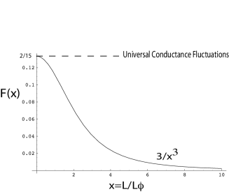
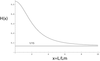
Figure 1: Function $F(x=L/L_{\phi})$ describing the scaling of the variance of the conductance distribution without magnetic impurities : see eq. (3). The function $H(x)$ represented on the right of the figure, describes the scaling of this variance when magnetic impurities are present, and a new dephasing length $L_{m}$ appears : see eq. (5).

For an infinite dephasing length scale ($x=0$), we recover the universal conductance value $\left<(\delta G)^{2}\right>_{V}=s^{2}\frac{2}{15}$, whereas $\left<(\delta G)^{2}\right>_{V}$ vanishes as expected in the classical limit $L\gg L_{\phi}$.

In the presence of magnetic impurities, the conductance $G$ is now a function of both the configuration of scalar potential $V({\bf r})=\sum_{i}v_{i}\delta({\bf r}-{\bf r}_{i})$ and the configuration of frozen spins $\{S_{i}\}$. For a given configuration of spin $\{S_{i}\}$, we can consider the distribution of $G(V,\{S_{i}\})$ as $V$ varies. This distribution $P_{V}(G(\{S_{i}\}))$ is still gaussian and independent of the configuration of spins. The length dependence of its variance is modified by the presence of the symmetry breaking disorder. A new magnetic dephasing length $L_{m}$ appears (here given to order $J^{-1}$) :

$$L_{m}^{2}=\hbar D\left(4\pi n_{\rm imp}\rho_{0}J^{2}S^{2}\right)^{-1},$$ (4)

where $D$ is the diffusion coefficient in the sample, $n_{\rm imp}$ the density of impurities and $\rho_{0}$ the electron’s density of states. In the limit $L_{m},L\ll L_{\phi}$, the variance of $P_{V}(G)$ reads

$$\left<\left[\delta G(\{S_{i}\})\right]^{2}\right>_{V} =H(L/L_{m})$$ (5)

$$=\frac{1}{4}F\left(0\right)+\frac{3}{4}F\left(\frac{2}{\sqrt{3}}\frac{L}{L_{m}}\right)+\frac{1}{4}F\left(\sqrt{2}\frac{L}{L_{m}}\right)+\frac{3}{4}F\left(\sqrt{\frac{2}{3}}\frac{L}{L_{m}}\right).$$

This function $H(x)$ is represented in figure 1 for $L_{\phi}\to\infty$.

We now focus on the dependence of this conductance on variations of the configurations of spins. For a given configuration of $V$, we consider the variation of conductance between two spin configurations (which differ by the orientation of the frozen spins $\{S_{i}\}$, but not their position) :

$$G\left(V,\{S_{j}^{(1)}\}\right)-G\left(V,\{S_{j}^{(2)}\}\right).$$ (6)

As $V$ is varied, this quantity fluctuates similarly to $G$. The corresponding distribution, obtained using the numerical Landauer method, is represented in Fig. 2 for several pairs of configurations $\{S_{j}^{(1)}\}$ and $\{S_{j}^{(2)}\}$.

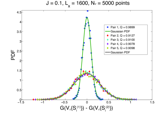
Figure 2: Distribution of the variation of conductance between two spin configurations $\{S_{j}^{(1)}\}$ and $\{S_{j}^{(2)}\}$ in a given sample $V$. These distributions are obtained using a numerical Landauer approach for the model (2) paulin1 . The coupling $J$ between the spins of the electron and the impurities was chosen as $J/t=0.1$, the system size was $40\times 1600$. For each configuration of spins, $5000$ configurations of scalar disorder $V$ were generated. The histograms over these $5000$ points are shown for $5$ pairs of spin configurations. While the distributions for pairs with a spin overlap $Q\simeq 0.91$ collapse within a good approximation, the distribution corresponding to $Q=0.99$ clearly deviates from these other distributions. This result illustrates the parameterisation of the distribution of $G\left(V,\{S_{j}^{(1)}\}\right)-G\left(V,\{S_{j}^{(2)}\}\right)$ by the spin overlap $Q$.

As expected, this distribution is still gaussian, with a vanishing average. For a fixed geometry, its variance appears to be parameterised by the overlap (1) between the two spin configurations : the distributions of $G$ for different pairs of configurations with similar overlap collapse. Indeed, its variance is entirely encoded by the average correlation between the conductances in two different frozen spin configurations $,\{S_{j}^{(1)}\}$ and $\{S_{j}^{(2)}\}$ :

$$(\Delta G)^{2}_{S^{(1)}S^{(2)}}=\left<\delta G\left(V,\{S_{j}^{(1)}\}\right)\delta G\left(V,\{S_{j}^{(2)}\}\right)\right>_{V},$$ (7)

where $\delta G(V,\{S_{j}^{(1)}\})=G(V,\{S_{j}^{(1)}\})-\langle G(V,\{S_{j}^{(1)}\})\rangle_{V}$. The length dependence of these correlations is obtained by extending (5) [Altshuler:1985, ; carpentier:2008, ]. In the same limit $L_{m}\ll L_{\phi}$ as in (5) , it reads

$$(\Delta G)^{2}_{S^{(1)}S^{(2)}} =\frac{1}{4}F\left(\sqrt{1-Q}\frac{L}{L_{m}}\right)+\frac{3}{4}F\left(\sqrt{1+\frac{Q}{3}}\frac{L}{L_{m}}\right)$$

$$+\frac{1}{4}F\left(\sqrt{1+Q}\frac{L}{L_{m}}\right)+\frac{3}{4}F\left(\sqrt{1-\frac{Q}{3}}\frac{L}{L_{m}}\right)$$ (8)

where $Q$ is the overlap between the two spin configurations defined in (1). This result is the starting point for our proposal to measure the overlap between random spin configurations : in a given sample when orientations of the spins are varied, the variations of the quantity (6) are entirely encoded by the overlap between the corresponding spin configuration. Such a measurement would allow for the first experimental determination of spin configuration’s overlap.

A crucial step needed to experimentally measure (6) is to sample the corresponding distribution. This distribution was defined by considering the statistics of $G$ when the potential $V$ is varied. However, one cannot vary the diffusing potential in a semiconducting spin glass without modifying completely the spin glass configuration ! We thus have to resort to the usual ergodic hypothesis of weak localisation (see Tsyplyatyev:2003 for a recent discussion). Following this hypothesis, the statistics of $G$ are usually determined experimentally by considering a magneto-conductance trace of a given metallic sample. When a flux is applied perpendicular to the sample, the conductance fluctuates in a random but reproducible way (see Fig. 3). The variance of the corresponding distribution approximates correctly the variance of the distribution $P_{V}(G)$ Tsyplyatyev:2003 .

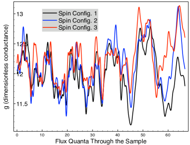
Figure 3: Magnetoconductance traces obtained by a numerical Landauer approach paulin1 . The different traces correspond to the same sample, i.e configuration of scalar disorder, but different configurations (i.e orientations) of the frozen spins.

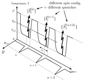
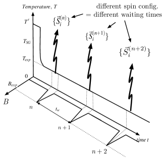
Figure 4: Proposed protocols to measure the correlations (overlap) between spin configurations corresponding to different quenches or different waiting times. In the first case, the different spins states $\{\vec{S}_{i}^{(n)}\}$ are labelled by the index of the quench $n$. All these states correspond to the spin configuration obtained after a time $t_{w}$ after entering the spin glass phase. At this time $t_{w}$, the spin configuration is sampled through the measurement of the corresponding magnetoconductance trace. The correlation between these traces gives access to the overlap between the corresponding spin states. In the second case, the spin configuration correspond to different waiting time $t_{w}^{(n)}$. Similarly, these states are probed through magnetoconductance measurements.

Following this line of reasoning, the proposed quantity to measure instead of (7) is

$$\langle\delta G(V,\{S_{j}^{(1)}\})\delta G(V,\{S_{j}^{(2)}\})\rangle_{B}=\\ \frac{1}{B_{\rm max}-B_{\phi}}\int_{B_{\phi}}^{B_{\rm max}}\delta G(V,\{S_{j}^{(1)}\},B)\delta G(V,\{S_{j}^{(2)}\},B)dB$$ (9)

A crucial approximation made in using (9) as an evaluation of (7) is the neglect of the spin glass response to the (weak) magnetic field. A crucial step in this possible experimental route would thus consist in determining the optimal maximum field $B_{\rm max}$ below which this spin glass response can be neglected, but high enough to provide the necessary sampling of the statistics of $G$.

In conclusion, we have proposed a first route to measurements of spin configurations overlap in metallic mesoscopic conductors. This route consist in determining the magneto-conductance traces for different spin configurations. The correlation between these traces gives access through eq. (2.3) to the overlap between the corresponding spin configurations. In a spin glass, these different spin configurations can be accessed either by successive cooling below the glass transition, or e.g by different waiting times. The proposed protocols corresponding to these two situations are illustrated in Fig. 4.

3 Anderson localisation with cold atoms

3.1 Introduction

The field of ultracold atoms has emerged in recent years as a new research field at the frontier between atomic, molecular and optical physics and condensed matter physics.  jaksch05_coldatoms ; lewenstein07_coldatoms_review ; bloch08_manybody . Trapping potentials of arbitrary shapes can be Fourier-synthesised via the superposition of different laser standing waves. In particular a single standing wave confines the atoms into planes, with negligible inter-plane coupling (over the time duration of the experiments, typically 100ms-1s); two orthogonal standing waves confine the atoms into tubes, while three standing waves create a cubic optical lattice. More sophisticated lattice geometries can be then achieved by superposing further spatial Fourier components. Hence optical potentials give unprecedented access to low-dimensional quantum systems and to arbitrary lattice Hamiltonians. When ultracold atoms are loaded in the lowest band of optical lattices, their physics is faithfully described by Bose- and Fermi-Hubbard models. The depth of the optical lattice allows to control the inter-site hopping, and hence the relevance of interactions against the kinetic energy over several orders of magnitude. Interactions are generally short-ranged (on-site only), and can be further tuned with the use of Feshbach resonances  roberts98_feshbach_rb . Hence experiments can span all regimes of lattice Hamiltonians, from the weakly interacting one to the strongly interacting one, and probe fundamental phenomena such as the onset of Mott insulating physics and the suppression of quantum coherence Greineretal02 ; Schneideretal08 .

Yet cold atomic samples contain typically $10^{5}-10^{6}$ atoms; when standing waves are applied to divide the system into planes or tubes, each layer/tube contains typically $10^{3}-10^{4}$ / 10-100 atoms respectively. Hence trapped cold atoms can be viewed as a particular instance of mesoscopic systems huang_meso , where the finite system size, dictated by a global (parabolic) trapping imposed on the atoms, can be far exceeded by the quantum coherence length. Coherent quantum many-body phenomena out of equilibrium can be probed in the system via a real-time control on the Hamiltonian parameters, and they have been demonstrated in recent experiments on Bloch oscillations in periodic lattices Dahanetal96 , Josephson oscillations in a double-well potential Albiezetal05 , coherent dipole oscillations in a parabolic trap Fertigetal05 , transitions from integrability to non-integrability kinoshita_cradle , etc.

Our recent theoretical activities on mesoscopic aspects of trapped cold atoms have been focused on the physics of Anderson localisation anderson_localisation of interacting bosonic atoms. Anderson localisation of interacting bosons is a long-standing problem in condensed matter physics fisher_boson_loc , and various experimental realizations have been attempted with ⁴He in a porous medium such as Vycor, aerogels or xerogels chan_vycor_localization or with disordered Josephson junctions vanoudenaarden_josephson_localization . However an experimental test of fundamental theoretical predictions is still lacking. Thanks to the flexibility in designing the trapping potential, cold atomic systems offer the possibility to explore one dimensional geometries, in which strong localisation effects are dramatic mott_loc and have been extensively studied theoretically lifshitz_desordonne . Moreover, the use of optical lattices and Feshbach resonances allow to study the interplay of disorder and a continuously tuned interaction.

Two methods to realise a controlled random (or pseudo-random) optical potential are currently available. One consists of imaging a disordered diffusive plate onto the atomic sample, thus creating a so-called laser-speckle potential lye05_speckle ; fort05_speckle1d ; clement_disorder_quasi_1D ; clement06_speckles . The reduction of the speckle size below the bosonic healing length has recently allowed to clearly observe real-space signatures of Anderson localisation on the density profile of a highly dilute gas expanding in a one-dimensional speckle potential billy_loc . The second method, to which our recent investigations have been devoted, is specific of optical lattice systems, and it is based on superposing a dominant (primary) standing wave with a secondary standing wave with an incommensurate period with respect to the primary one. In this way a quasi-periodic superlattice is created, whose physics interpolates between the one of a random system and the one of a perfectly periodic potential, as we will discuss in the next section. This approach has also allowed to recently observe clear signatures of Anderson localisation in expanding one-dimensional atomic clouds with negligible interaction roati_loc , as well as signatures of unconventional insulating behaviour in the strongly correlated regime fallani07_boseglass .

3.2 Ultracold bosonic atoms in disordered optical lattices

Interacting bosons loaded in a deep optical lattice plus a random potential are described by a Bose-Hubbard Hamiltonian jaksch_bose_hubbard , of the form

$$H=-J\sum_{\langle ij\rangle}(b^{\dagger}_{i}b_{j}+\mathrm{H.c.})+\frac{U}{2}\sum_{i}n_{i}(n-1)+\sum_{i}(\epsilon_{i}-\mu)n_{i},$$ (10)

where $b_{i}$ is the boson annihilation operator, $n_{i}=b^{\dagger}_{i}b_{i}$ is the boson number operator, $J$ is the hopping integral, $U$ is the on-site boson-boson repulsion, $i$ runs over the sites of an optical lattice, and $\langle ij\rangle$ runs over the pairs of nearest neighbouring sites. $\epsilon_{i}$ is the on-site energy, accounting for the overall trapping potential (of the form $V_{t}(i-i_{0})^{2}$) and for any additional random or quasi-random potential.

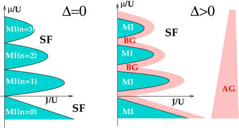
Figure 5: Schematic phase diagram of the Bose Hubbard model without disorder (left panel) and with disorder (right panel). MI=Mott insulator, SF=superfluid, BG=Bose glass, AG=Anderson glass.

In absence of additional potentials, the Bose-Hubbard model at zero temperature features a gapless superfluid (SF) phase with long-range phase coherence for large $J/U$; lowering this ratio leads the system to a quantum phase transition towards gapped Mott-insulating (MI) phases at integer fillings and with short-range coherence. (see Fig. 5). Upon introducing a random on-site potential, namely taking $\epsilon_{i}$ as a random variable in the interval $[-\Delta/2,\Delta/2]$, two new phases appear: for large $J/U$, an Anderson glass (AG) phase, in which weakly interacting particles are Anderson-localised by disorder, and their state connects continuously with that of the single-particle localisation problem; in the strongly interacting regime (low $J/U$ ratio), a Bose glass (BG) phase, characterised by Anderson localisation of collective modes of the system, which can be essentially pictured as particle-hole excitations involving localised quasi-particle states. Both AG and BG are exotic insulators compared to the MI, in that they feature a gapless spectrum and a finite compressibility in absence of long-range coherence. The schematic phase diagrams of Fig. 5 can be obtained via mean-field theory fisher_boson_loc and have been repeatedly confirmed via numerically exact techniques, such as quantum Monte Carlo (QMC) ProkofevS98 and density matrix renormalization group (DMRG) Rapschetal99 .

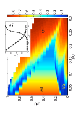
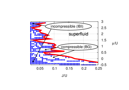
Figure 6: Phase diagrams for the Bose-Hubbard model in a Harper potential. Left panel: phase diagram for weak disorder $\Delta/U=0.1$ (in the inset the superfluid fraction and the compressibility gap are plotted as functions of $t/U$ for $\mu/U=0.25$). Right panel: phase diagram for strong disorder, $\Delta/U=0.5$.

In the case of a quasi-periodic superlattice, the on-site potential takes the form of a Harper potential $\epsilon_{i}=\Delta\cos(2\pi\alpha i+\phi)$ where $0<\alpha<1$ is an irrational number and $\phi$ an arbitrary phase factor. In the following we will specialise the discussion to one-dimensional systems, for which the problem of a single quantum particle in the Harper potential has been the subject of extensive investigations in the past Sokoloff85 . A one-dimensional particle in a purely random potential (as the one described above) is known to undergo Anderson localisation in all its energy eigenstates for any infinitesimal disorder strength, namely the Anderson transition occurs at $\Delta=0$. Moreover the single-particle density of states is continuous (on average over the disorder realizations). On the contrary a single particle in the Harper potential undergoes an Anderson transition from all extended to all localised eigenstates for a finite disorder, $\Delta=2J$ Aubry_harper . The density of states is not continuous (even upon averaging over the arbitrary phase $\phi$), and it is structured in bands both on the extended and on the localised side of the transition.

Our investigations have been focused on effect of strong interactions on the localisation phenomena of bosons in a Harper potential, following a setup which has been recently realised in optical lattice experiments fallani07_boseglass . Making use of numerical exact diagonalisation, QMC and DMRG methods, as well as of analytical bosonization techniques, we have addressed the fundamental questions on the topology of the phase diagram in presence of a quasi-random potential Roscilde08 ; Dengetal08 . Fig 6 shows the phase diagram of the Hubbard model in the Harper potential for two values of the disorder potential $\Delta/U=0.1$ (obtained via DMRG) and $\Delta/U=0.5$ (obtained via QMC), and for $\alpha=830/1076$, which is chosen as the ratio of the wavelengths used in the experimental realization, Ref.  fallani07_boseglass . In the case of weaker disorder ( $\Delta/U=0.1$) one observes the appearance of a Bose-glass phase with vanishing superfluid density and finite compressibility at the interface between the conventional Mott insulating and superfluid phase. Yet, at variance with the case of a truly random potential ProkofevS98 ; Rapschetal99 , a direct transition is possible between SF and MI close to the tip of the Mott lobe (as shown in the inset of Fig. 6). This fact is intimately related with the existence of a finite localisation threshold associated with the quasiperiodic potential: analogously to what happens at the single particle level, when the intersite hopping exceeds a critical value the quasiperiodic potential has no localising effect on the collective modes of the system, so that the Bose-glass phase is not observed, and a conventional phase transition between MI and SF can take place with the onset of gapless and propagating collective modes. The single-particle localisation threshold $\Delta=2J$ is attained for $J/U=0.2$, which is already to the left of the Mott-lobe tip; on the other hand interactions play the role of screening the quasi-periodic potential, so that even a smaller $J$ is expected to mark the disappearance of the Bose glass. This is quantitatively consistent with our data, where the BG phase seems to disappear for $J/U\approx 0.15$.

On the opposite side of the spectrum, a very strong quasi-periodic potential has the effect of fully destabilising the MI phase of the homogeneous system at integer fillings; indeed for $\Delta/U=0.5$ the amplitude of the fluctuations of the Harper potential ($\sim U$) overcome the gap characteristic of the MI phase, which is upper-bounded by $U$. Hence the MI phase disappears from the phase diagram, substituted by novel insulating phases stabilised by the quasi-periodic potential. Such phases reflect the intermediate nature of the quasi-periodic potential: in fact gapless and incoherent BG regions alternate with gapped incommensurate-band-insulator (IBI) regions, which are the quasi-periodic analog of conventional band insulators appearing in interacting bosonic models in a commensurate superlattice Rousseauetal06 . In the limit of a deep quasiperiodic potential, the IBI phase can be associated to the opening of a finite gap for addition of a particle in any of the potential wells of the Harper potential: in this case an incommensurate ”shell” of localised state is filled, and to start filling the next shell a gap needs to be overcome. This phenomenon does not occur in the case of a truly random potential, because the potential wells are not bounded in size, and hence the ”charging energy” of each well can be arbitrarily small, making the system gapless at all fillings.

3.3 Detecting disorder-induced phases

The above results show that a very rich showcase of quantum phases can be implemented by experiments with strongly interacting bosons in incommensurate optical superlattices. Nonetheless the fundamental question remains on how one can detect experimentally the occurrence of such phases and all the details of complicated phase diagrams. This question is ultimately related with the potential use of these physical systems as analog quantum simulators feynman82_simulators , capable of providing the answer to open theoretical questions concerning models which are implemented literally in the experiment.

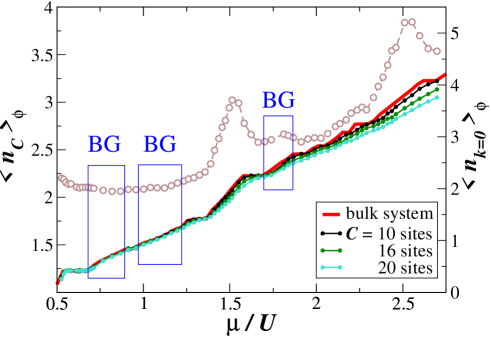
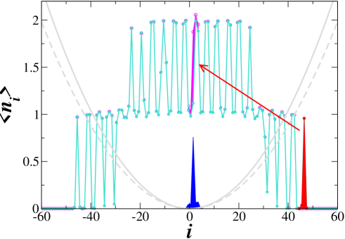
Figure 7: Trap-squeezing detection of Bose glass phases. Upper panel: average central density and coherent fraction as a function of the chemical potential (controlled by the trapping potential Roscilde09 ) for a system of $N=100$ trapped bosons in an incommensurate superlattice with $\Delta=U/2=10J$ and $\alpha=830/1076$; boxed regions show BG behaviour, namely finite compressibility without any significant increase in the coherence. Lower panel: trap-squeezing-induced migration of a particle from a localised state on the trap wings from a localised state in the trap centre. The shown data refer to a variation of the trapping potential $V_{t}$ from $0.013J$ to $0.014J$.

In the specific case of novel insulators induced by quasi-disordered potentials, our recent activity has been focused on how to detect their most striking feature, namely the simultaneous absence of a gap and of long-range phase coherence Roscilde09 . In particular the gapless excitations of a BG are particle excitations, hole excitations, and particle-hole ones, and they are probed directly by the compressibility, which is indeed finite in the BG phase. The trapping potential confining the atoms offers the possibility of probing the compressibility by studying the response of the system to the increase of the trapping frequency (”trap squeezing”). Indeed such an operation tries to push particles from the trap wings towards the centre, where new particles are accepted only if the local state of the system has a vanishing gap to particle addition. Hence measuring a finite response of the average density in the centre of the trap upon increasing the trap frequency amounts to probing the realization of a locally compressible phase in the trap centre.

Knowing that this phase actually corresponds to a BG requires the additional information on short-range coherence. The phase coherence of trapped cold atoms can be measured with time-of-flight measurements, which reveal the momentum distribution and in particular the zero-momentum component (coherent fraction):

$$n_{k=0}=\frac{1}{N}\sum_{ij}\langle b_{i}^{\dagger}b_{j}\rangle,$$ (11)

where $N$ is the total particle number. In particular, if a particle is added to a BG phase, it will occupy a Anderson localised quasi-particle state, and hence it will not increase the coherent fraction of the system. Consequently a BG phase realised in the centre of the trap should be identified with a finite response of the central density to trap squeezing and on the simultaneous absence of response in the coherent fraction. This is indeed what it is observed in QMC simulations on trapped bosons subject to a variable trapping potential, as shown in Fig. 7. The realization of such a behaviour occurs for values of the chemical potential which correspond to BG behaviour of the homogeneous system, so that this type of measurement allows to reconstruct the phase diagram of the system in absence of the trap. The major requirement of this proposal is the measurement of the average density over a region of a linear size of $5-10\mu$m, corresponding to 10-20 lattice sites. This is indeed possible with current large-aperture optics Sortaisetal07 .

References

- [1] A. H. Castro Neto, F. Guinea, N. M. R. Peres, K. S. Novoselov, and A. K. Geim, (2009) ‘The electronic properties of graphene’ Rev. Mod. Phys. 81, 109.
- [2] A. K. Geim and K. S. Novoselov, (2007) ‘The rise of graphene’ Nature Materials 6:183.
- [3] J.-C. Charlier, X. Blase, and S. Roche, (2007) ‘Electronic and transport properties of nanotubes’ Rev. Mod. Phys., 79:677.
- [4] S. Ijima, (1991) ‘Helical microtubules of graphitic carbon’ Nature (London), 354:56.
- [5] R. Hanson, L. P. Kouwenhoven, J. R. Petta, S. Tarucha, and L. M. K. Vandersypen, (2007) ‘Spins in few-electron quantum dots’ Rev. Mod. Phys., 79:1217.
- [6] I. Bloch, J. Dalibard, and W. Zwerger, (2008) ‘Many-body physics with ultracold gases’ Rev. Mod. Phys., 80:885.
- [7] P. W. Anderson, (1958) ‘Absence of diffusion in certain random lattices’ Phys. Rev., 109:1492.
- [8] N. F. Mott and W. D. Twose, (1961) ‘The theory of impurity conduction’ Adv. Phys., 10:107.
- [9] E. Abrahams, P. W. Anderson, D. C. Licciardello, and T. V. Ramakrishnan, (1979) ‘Scaling Theory of Localization: Absence of Quantum Diffusion in Two Dimensions’ Phys. Rev. Lett., 42:673.
- [10] C. W. J. Beenakker, (1997) ‘Random-matrix theory of quantum transport’ Rev. Mod. Phys., 69:731.
- [11] T. Roscilde, (2008) ‘Bosons in one-dimensional incommensurate superlattices’ Phys. Rev. A, 77:063605.
- [12] T. Roscilde, (2009) ‘Probing correlated phases of bosons in optical lattices via trap squeezing’ New J. of Physics, 11, 023019.
- [13] G. Paulin and D. Carpentier, (2009) Numerical Landauer study of coherent electronic transport with random magnetic fields. preprint.
- [14] D. Carpentier and E. Orignac, (2008) ‘Measuring overlaps in mesoscopic spin glasses via conductance fluctuations’ Phys. Rev. Lett., 100:057207.
- [15] X. Deng, R. Citro, A. Minguzzi, , and E. Orignac, (2008) ‘Phase diagram and momentum distribution of an interacting Bose gas in a bichromatic lattice’ Phys. Rev. A, 78:013625.
- [16] M. P. A. Fisher, P. B. Weichman, G. Grinstein, and D. S. Fisher, (1989) ‘Boson localization and the superfluid-insulator transition’ Phys. Rev. B, 40:546.
- [17] F. Guerra, (2002) ‘Broken replica symmetry bounds in the mean field spin glass model’ Comm. Math. Phys., 233:1.
- [18] G. Parisi, (1980) ‘The order parameter for spin glasses: a function on the interval 0-1’ J. Phys. A, 13:1101.
- [19] M. Talagrand, (2006) ‘The Parisi formula’ Ann. of Math., 163:221.
- [20] M. Mézard, G. Parisi, and M. Virasoro, (1987) Spin Glass Theory and Beyond. World Scientific.
- [21] G. Parisi, (2006) ‘Mean field theory of spin glasses: statics and dynamics’ In J.-P. Bouchaud, M. Mézard, and J. Dalibard, editors, Complex Systems, Les Houches Summer School, volume LXXXV.
- [22] E. Akkermans and G. Montambaux, (2007) Mesoscopic Physics of electrons and photons, Cambridge University Press.
- [23] M. Albiez, R. Gati, J. Fölling, S. Hunsmann, M. Cristiani, and M. K. Oberthaler, (2005) ‘Direct observation of tunneling and nonlinear self-trapping in a single bosonic Josephson junction’ Phys. Rev. Lett., 95:010402.
- [24] G.B. Alers, M.B. Weissman, and N.E. Israeloff, (1992) ‘Mesoscopic tests for thermally chaotic states in a Cu:Mn spin glass’ Phys. Rev. B, 46:507.
- [25] B.L. Al’tshuler and B.Z. Spivak, (1985) ‘Variation of the random potential and the conductivity of samples of small dimensions’ JETP Lett., 42:447.
- [26] S. Aubry and G. André, (1980) ‘Analyticity breaking and Anderson localization in incommensurate lattices’ Ann. Isr. Phys. Soc., 3:113.
- [27] J. Billy, V. Josse, Z. Zuo, A. Bernard, B. Hambrecht, P. Lugan, D. Clement, L. Sanchez-Palencia, P. Bouyer, and A. Aspect. ‘Direct observation of Andersen localization of matter waves in a controlled disorder’ Nature (London), 453:891, 2008.
- [28] J.-P. Bouchaud, (1992) ‘Weak ergodicity breaking and aging in disordered systems’ J. Phys. I, 2:1705.
- [29] A.J. Bray and M.A. Moore, (1986) In L. van Hemmen and I. Morgenstein, editors, Heidelberg Colloquium on Glassy Dynamics and Optimization. Springer-Verlag.
- [30] M. H. W. Chan, K. I. Blum, S. Q. Murphy, G. K. S. Wong, and J. D. Reppy, (1988) ‘Disorder and the superfluid transition in liquid 4He’ Phys. Rev. Lett., 61:1950, 1988.
- [31] D. Clément, A. F. Varón, M. Hugbart, J. A. Retter, P. Bouyer, L. Sanchez-Palencia, D. M. Gangardt, G. V. Shlyapnikov, and A. Aspect, (2005) ‘Suppression of transport of an interacting elongated Bose-Einstein condensate in a random potential’ Phys. Rev. Lett., 95:170409.
- [32] D. Clément, A. F. Varón, J. A. Retter, L. Sanchez-Palencia, A. Aspect, and P. Bouyer, (2006) ‘Experimental study of the transport of coherent interacting matter-waves in a 1d random potential induced by laser speckle’ New Journal of Physics, 8:165.
- [33] L. Cugliandolo, (2002) ‘Dynamics of glassy systems’ In Lecture notes, Les Houches, Elsevier, 2002.
- [34] M. Ben Dahan, E. Peik, J. Reichel, Y. Castin, and C. Salomon (1996) ‘Bloch oscillations of atoms in an optical potential’ Phys. Rev. Lett., 76:4508.
- [35] P.G.N. de Vegvar, L.P. Lévy, and T.A. Fulton, (1991) ‘Conductance fluctuations of mesoscopic spin glasses’ Phys. Rev. Lett., 66:2380.
- [36] L. Fallani, J. E. Lye, V. Guarrera, C. Fort, and M. Inguscio, (2007) ‘Ultracold atoms in a disordered crystal of light: Towards a Bose glass’ Phys. Rev. Lett., 98:130404.
- [37] S. Feng, A. Bray, P. Lee, and M. Moore, (1987) ‘Universal conductance fluctuations as a probe of chaotic behavior in mesoscopic metallic spin glasses’ Phys. Rev. B, 36:5624.
- [38] C. D. Fertig, K. M. O’Hara, J. H. Huckans, S. L. Rolston, W. D. Phillips, , and J. V. Porto, (2005) ‘Strongly inhibited transport of a degenerate 1d Bose gas in a lattice’ Phys. Rev. Lett., 94:120403.
- [39] R. P. Feynman, (1982) Simulating Physics with Computers, International Journal of Theoretical Physics, 21:467.
- [40] D. S. Fisher and D. A. Huse, (1986) ‘Ordered phase of short-range Ising spin-glasses’ Phys. Rev. Lett., 56:1601.
- [41] C. Fort, L. Fallani, V. Guarrera, J. E. Lye, M. Modugno, D. S. Wiersma, and M. Inguscio, (2005) ‘Effect of optical disorder and single defects on the expansion of a Bose-Einstein condensate in a one-dimensional waveguide’ Phys. Rev. Lett., 95:170410.
- [42] M. Greiner, O. Mandel, T. Esslinger, T.W. Hänsch, , and I. Bloch, (2002) ‘Quantum phase transition from a superfluid to a Mott insulator in a gas of ultracold atoms’ Nature (London), 415:39.
- [43] K. Huang, (2000) ‘Cold trapped atoms: A mesoscopic system’ invited talk at the third joint meeting of Chinese physicists worldwide, Chinese University of Hong Kong.
- [44] N.E. Israeloff, M.B. Weissman, G.J. Nieuwenhuys, and J. Kosiorowska, (1989) ‘Electrical noise from spins fluctuations in Cu:Mn’ Phys. Rev. Lett., 63:794.
- [45] D. Jaksch, C. Bruder, J. I. Cirac, C. W. Gardiner, and P. Zoller, (1998) ‘Cold Bosonic Atoms in Optical Lattices’ Phys. Rev. Lett., 81:3108.
- [46] D. Jaksch and P. Zoller, (2005) ‘The cold atom Hubbard toolbox’ Ann. Phys. (N. Y.), 315:52.
- [47] J. Jaroszynski, J. Wrobel, G. Karczewski, T. Wojtowicz, and T. Dietl, (1998) ’Magnetoconductance noise and irreversibilities in submicron wires of spin-glass n+-CdMnTe’ Phys. Rev. Lett., 80:5635.
- [48] T. Kinoshita, T. Wenger, and D. S. Weiss, (2006) ‘A quantum Newton’s cradle’ Nature (London), 440:900.
- [49] M. Lewenstein, A. Sanpera, V. Ahufinger, B. Damski, A. Sen De, and U. Sen, (2007) ‘Ultracold atomic gases in optical lattices: mimicking condensed matter physics and beyond’ Ann. Phys. (N. Y.), 56:243.
- [50] I. M. Lifshitz, L. P. Pastur, and S. Gredeskul, (1988) Introduction to the theory of disordered systems, Wiley and Sons, New York.
- [51] J. E. Lye, L. Fallani, M. Modugno, D. S. Wiersma, C. Fort, and M. Inguscio, (2005) ‘Bose-Einstein condensate in a random potential’ Phys. Rev. Lett., 95:070401.
- [52] K.A. Meyer and M.B. Weissman, (1995) ‘Mesoscopic electrical noise from spins in Au:Fe’ Phys. Rev. B, 51:8221.
- [53] G. Neuttiens, J. Eom, C. Strunk, H. Pattyn, C. Van Haesendonck, Y. Bruynseraede, and V. Chandrasekhar, (1998) ‘Thermoelectric effects in mesoscopic Au:Fe spin-glass wire’ Europhys. Lett., 42:185.
- [54] G. Neuttiens, C. Strunk, C. Van Haesendonck, and Y. Bruynseraede, (2000) ‘Universal conductance fluctuations and low-temperature 1/f noise in mesoscopic Au:Fe spin glasses’ Phys. Rev. B, 62:3905.
- [55] M. Pascaud and G. Montambaux, (1998) ‘Interference effects in mesoscopic disordered rings and wires’ Physics - Uspekhi, 41:182, 1998.
- [56] N. V. Prokof’ev and B. V. Svistunov, (1998) ‘Comment on “one-dimensional disordered bosonic Hubbard model: A density-matrix renormalization group study’ Phys. Rev. Lett., 80:4355.
- [57] S. Rapsch, U. Schollwöck, and W. Zwerger, (1999) ‘Density matrix renormalization group for disordered bosons in one dimension’ Europhys. Lett., 46:559.
- [58] G. Roati, C. D’Errico, L. Fallani, M. Fattori, C. Fort, M. Zaccanti, G. Modugno, M. Modugno, and M. Inguscio, (2008) ‘Anderson localization of a non-interacting Bose-Einstein condensate’ Nature (London), 453:895.
- [59] J. L. Roberts, N. R. Claussen, James P. Burke, Jr., Chris H. Greene, E. A. Cornell, and C. E. Wieman, (1998) ‘Resonant magnetic field control of elastic scattering in cold 85Rb’ Phys. Rev. Lett., 81:5109.
- [60] V. G. Rousseau, D. P. Arovas, M. Rigol, F. Hébert, G. G. Batrouni, , and R. T. Scalettar, (2006) ‘Exact study of the one-dimensional boson Hubbard model with a superlattice potential’ Phys. Rev. A, 73:174516.
- [61] U. Schneider, L. Hackermüller, S. Will, Th. Best, T. A. Costi I. Bloch, R. W. Helmes, D. Rasch, , and A. Rosch, (2008) ‘Metallic and insulating phases of repulsively interacting fermions in a 3d optical lattice’ Science, 322:520.
- [62] J.B. Sokoloff, (1985) ‘Unusual band structure, wave functions electrical conductance in crystals with incommensurate periodic potentials’ Phys. Rep., 126:189.
- [63] Y. R. P. Sortais, H. Marion, C. Tuchendler, A. M. Lance, M. Lamare, P. Fournet, C. Armellin, R. Mercier, G. Messin, A. Browaeys, and P. Grangier, (2007) ‘Diffraction-limited optics for single-atom manipulation’ Phys. Rev. A, 75:013406.
- [64] O. Tsyplyatyev, I.L. Aleiner, V.I. Fal’ko, and I.V. Lerner, (2009) ‘Applicability of the ergodic hypothesis to mesoscopic fluctuations’ Phys. Rev. B, 68:121301.
- [65] A. van Oudenaarden, S . J. K. Várdy, and J.E. Mooij, (1996) ‘One-dimensional localization of quantum vortices in disordered Josephson junction arrays’ Phys. Rev. Lett., 77:4257.
- [66] M.B. Weissman, (1993) ‘What is a spin glass ? a glimpse via mesoscopic noise’ Rev. Mod. Phys., 65:829.