Near-field intensity correlations in parametric photoluminescence from a planar microcavity

Abstract

We study the spatio-temporal pattern of the near-field intensity correlations generated by parametric scattering processes in a planar optical cavity. A generalized Bogolubov-de Gennes model is used to compute the second order field correlation function. Analytic approximations are developed to understand the numerical results in the different regimes. The correlation pattern is found to be robust against a realistic disorder for state-of-the-art semiconductor systems.

I Introduction

Quantum correlations in many-body and optical systems are playing a crucial role in a variety of fields, from the microscopic study of novel states of matter in quantum fluids Pitaevskii and Stringari (2003); Bloch et al. (2008), to the control and suppression of noise in optical systems Lugiato et al. (1998); Gatti et al. (2009); Zambrini et al. (2000); Lopez et al. (2008); Delaubert et al. (2008), to the exploration of analog models of gravitational and cosmological systems Balbinot et al. (2008); Carusotto et al. (2008, 2009).

In this perspective, non-linear optical systems exhibit a rich variety of phenomena Butcher and Cotter (1993); Walls and Milburn (1994), involving the interplay of parametric scattering with losses, non-linear energy shifts, and the peculiar dispersion of light in confined geometries. As a most significant example of this physics, an example of phase transition of the Bose-Einstein class has recently started being investigated in the optical parametric oscillation in planar geometries Savvidis et al. (2000); Ciuti et al. (2003).

Theoretical work has suggested that further insight in this physics can be obtained from the spatial and temporal pattern of correlations of the emitted light Carusotto and Ciuti (2005); Drummond and Dechoum (2005): as the critical point for parametric oscillation is approached, the correlation length and time of the parametric emission show a divergence that is closely related to the one of thermodynamical phase transitions.

To this purpose, semiconductor microcavities in the strong coupling regime appear as most favorable systems Savvidis et al. (2000); Ciuti et al. (2003); Deveaud (2005) as they are intrinsically grown with a planar geometry, and nonlinear interactions between the dressed photons – the so-called polaritons – are remarkably strong. First experiments demonstrating quantum correlations have recently appeared Savasta et al. (2005); Baas et al. (2006); Romanelli et al. (2007).

In the present work, we investigate the physics of the intensity correlations that are generated by parametric scattering processes. Depending on the pump frequency and intensity, different regimes can be identified. In addition to the usual short-distance correlations that are generally present in any interacting system, spontaneous parametric emission processes are responsible for additional long-distance ones, whose correlation length diverges as the optical parametric oscillation threshold is approached. In addition to their intrinsic interest, an experimental study of intensity correlation in this simplest system will open the way to the investigation of more complex geometries that in many aspects mimic the behavior of quantum fields in curved space-times Marino (2008).

Our approach is based on a generalized, non-equilibrium Bogolubov-de Gennes approximation in which weak fluctuations around the classical coherent field are described in terms of a quadratic Hamiltonian Castin (2001); Ciuti et al. (2003); Verger et al. (2007); Sarchi et al. (2009). Solving in frequency space the corresponding quantum Langevin equations allows to obtain predictions for the spatial and temporal dependence of the in-cavity intensity correlations. These then directly transfer to the near-field correlations of the emitted light. The study of the simplest planar geometry is extended to the more realistic case of weakly disordered systems: in this regime, the effect of disorder is shown not to qualitatively modify the peculiar correlation pattern.

In Section II, we review the theoretical formalism based on the Bogolubov approximation and we discuss how correlations transfer from the in-cavity field to the emitted radiation. In Section III.A we present the numerical results for a one-dimensional, spatially uniform case. Approximate analytical calculations are presented in Section III.B and used to physically interpret the numerical results. Numerical results for a two-dimensional disordered system are discussed in Section IV. Conclusions are drawn in Section V.

II Formalism

In this section we briefly review the formalism which will be used to calculate the intensity correlations of the emitted light. As we are restricting to the case of small fluctuations around a strong coherent field, a Bogolubov approach is adapted to describe the dynamics of quantum fluctuations. In the simplest case of a spatially homogeneous geometry the Bogolubov equations can be worked out to analytical expressions for the physical observables. In the general case, numerical results can be obtained by inverting the Bogolubov matrix for the specific geometry under investigation.

II.1 The system Hamiltonian

We describe the exciton and the photon quantum fields $\hat{\Psi}_{x}({\bf r})$ and $\hat{\Psi}_{c}({\bf r})$ as scalar Bose fields. The Hamiltonian is the sum of terms describing the free propagation of excitons and photons $\hat{H}_{0}$, their dipole coupling $\hat{H}_{R}$, the two-body exciton-exciton interaction $\hat{H}_{X}$, saturation of the exciton-photon coupling $\hat{H}_{s}$ and the external pumping $\hat{H}_{p}$ Ciuti et al. (2003); Carusotto and Ciuti (2004):

$$\hat{H}=\hat{H}_{0}+\hat{H}_{R}+\hat{H}_{x}+\hat{H}_{s}+\hat{H}_{p}.$$ (1)

The free propagation term has the form

$$\hat{H}_{0} = \int d^{2}{\bf r}\hat{\Psi}^{\dagger}_{x}({\bf r})[E_{x}-(\hbar^{2}/2m_{x})\nabla^{2}+U_{x}({\bf r})]\hat{\Psi}_{x}({\bf r})$$ (2)

$$+ \int d^{2}{\bf r}\hat{\Psi}^{\dagger}_{c}({\bf r})[\epsilon_{c}(-i\vec{\nabla})+U_{c}({\bf r})]\hat{\Psi}_{c}({\bf r})$$

where $E_{x}$ is the exciton energy, $m_{x}$ its effective mass, and $\epsilon_{c}$ is the photon dispersion in the planar cavity; $U_{x,c}$ are the external potentials acting on respectively the photon and the exciton. The dipole exciton-photon coupling has the form

$$\hat{H}_{R}=\hbar\Omega_{R}\int d^{2}{\bf r}[\hat{\Psi}^{\dagger}_{x}({\bf r})\hat{\Psi}_{c}({\bf r})+\textrm{h.c.}]$$ (3)

and is quantified by the Rabi frequency $\Omega_{R}$. The effective two-body exciton-exciton interaction term

$$\hat{H}_{x}=\frac{1}{2}g_{x}\int d^{2}{\bf r}\hat{\Psi}^{\dagger}_{x}({\bf r})\hat{\Psi}^{\dagger}_{x}({\bf r})\hat{\Psi}_{x}({\bf r})\hat{\Psi}_{x}({\bf r})$$ (4)

models both Coulomb interaction and the effect of Pauli exclusion on electrons and holes Rochat et al. (2000); Ben-Tabou de Leon and Laikhtman (2001).

$$\hat{H}_{s}=g_{s}\int d^{2}{\bf r}[\hat{\Psi}^{\dagger}_{c}({\bf r})\hat{\Psi}^{\dagger}_{x}({\bf r})\hat{\Psi}_{x}({\bf r})\hat{\Psi}_{x}({\bf r})+\textrm{h.c.}]$$ (5)

is the term modeling the saturation of the exciton oscillator strength Rochat et al. (2000). The external pump term has the form

$$\hat{H}_{p}=\hbar\int d^{2}{\bf r}[\hat{\Psi}^{\dagger}_{c}({\bf r})\,F_{p}({\bf r},t)+\textrm{h.c.}]\,.$$ (6)

In the following of the paper, we assume that the system is driven by a continuous-wave monochromatic pump with a plane wave spatial profile

$$F({\bf r},t)=e^{-i\omega_{p}t}e^{i{\bf k}_{p}\cdot{\bf r}}\,F_{0}.$$ (7)

Excitons and photons decay in time with a rate $\gamma_{x}$ and $\gamma_{c}$, respectively.

II.2 Bogolubov-de Gennes formalism

To make the problem analytically tractable, we perform the Bogolubov approximation Castin (2001): the two quantum fields are split into a strong coherent –classical– component and weak quantum fluctuations

$$\hat{\Psi}_{x(c)}({\bf r},t)=e^{-i\omega_{p}t}\left[\Phi_{x(c)}({\bf r})+\delta\hat{\psi}_{x(c)}({\bf r},t)\right].$$ (8)

This decomposition is then inserted into the Hamiltonian (1) and all terms of third and higher order in the fluctuations are neglected. This leads to a quadratic Hamiltonian for the fluctuation field that can be attacked with available theoretical tools.

The classical component ${\Phi}_{x(c)}({\bf r})$ is obtained from the Heisenberg equations of motion of the quantum field $\hat{\Psi}_{x(c)}({\bf r})$ by factorizing out the multi-operator averages. This leads to the following pair of generalized Gross-Pitaevskii equations:

$$\hbar\omega_{p}\Phi_{x}({\bf r}) = \left(-\frac{\hbar^{2}\nabla^{2}}{2m_{x}}+U_{x}({\bf r})-i\hbar\gamma_{x}/2+g_{x}\mid\Phi_{x}({\bf r})\mid^{2}\right.$$ (9)

$$+ \left.2g_{s}\mbox{Re}\left\{\Phi_{x}^{*}({\bf r})\Phi_{c}({\bf r})\right\}\right)\Phi_{x}({\bf r})$$

$$+ \left(\hbar\Omega_{R}+g_{s}\mid\Phi_{x}({\bf r})\mid^{2}\right)\Phi_{c}({\bf r}),$$

$$\hbar\omega_{p}\Phi_{c}({\bf r}) = \left[\epsilon_{c}(-i\vec{\nabla})+U_{c}({\bf r})-i\hbar\gamma_{c}/2\right]\Phi_{c}({\bf r})$$

$$+ \left(\hbar\Omega_{R}+g_{s}\mid\Phi_{x}({\bf r})\mid^{2}\right)\Phi_{x}({\bf r})+\hbar F_{0}e^{i{\bf k}_{p}\cdot{\bf r}}\,,$$

Note that the classical field $\Phi_{c,x}({\bf r})$ that is obtained from this equation does not include the correction due to the backaction of fluctuations onto the coherent component Castin and Dum (1997). To take this effect into account, one should include the contribution $\langle\delta\hat{\psi}^{\dagger}_{x}({\bf r})\,\delta\hat{\psi}_{x}({\bf r})\rangle$ of the fluctuating fields to the density and then iteratively solve (9-II.2) up to convergence. As in the present paper we are interested in the correlation properties of the field fluctuations, this effect can be safely neglected in what follows.

Within the input-output formalism Walls and Milburn (1994), the quantum dynamics of fluctuations can be written in terms of quantum Langevin equations of the form Ciuti and Carusotto (2006); Verger et al. (2007); Sarchi et al. (2009)

$$i\hbar\partial_{t}{\bf\delta\Psi}({\bf r},t)=\hat{M}\,{\bf\delta\Psi}({\bf r},t)+\hbar{\bf f}({\bf r},t)\,,$$ (11)

where

$${\bf\delta\Psi}=(\delta\psi_{x},\delta\psi_{x}^{\dagger},\delta\psi_{c},\delta\psi_{c}^{\dagger})^{T}$$ (12)

is the four-component quantum fluctuation field. The matrix $\hat{M}$ is obtained by linearizing the Heisenberg equation of motion for the quantum field around the classical component. In our case, it has the form:

$$\hat{M}=\left(\begin{array}[]{cccc}\hat{T}_{x}-i\frac{\hbar\gamma_{x}}{2}&\Sigma^{xx}_{12}&\tilde{\Omega}_{R}&\Sigma^{xc}_{12}\\ -(\Sigma^{xx}_{12})^{*}&-\hat{T}_{x}-i\frac{\hbar\gamma_{x}}{2}&-(\Sigma^{xc}_{12})^{*}&-\tilde{\Omega}_{R}\\ \tilde{\Omega}_{R}&\Sigma^{xc}_{12}&\hat{T}_{c}-i\frac{\hbar\gamma_{c}}{2}&0\\ -(\Sigma^{xc}_{12})^{*}&-\tilde{\Omega}_{R}&0&-\hat{T}_{c}-i\frac{\hbar\gamma_{c}}{2}\end{array}\right)\,,$$ (13)

with

$$\hat{T}_{x}({\bf r}) = -\frac{\hbar^{2}\nabla^{2}}{2m_{x}}+U_{x}({\bf r})-\hbar\omega_{p}+2g_{x}\mid\Phi_{x}({\bf r})\mid^{2}$$ (14)

$$+ 4g_{s}\mbox{Re}\{\Phi_{x}^{*}({\bf r})\Phi_{c}({\bf r})\}\,,$$

$$\hat{T}_{c}({\bf r}) = \epsilon_{c}(-i\vec{\nabla})+U_{c}({\bf r})\,,$$ (15)

$$\Sigma_{12}^{xx}({\bf r}) = g_{x}\Phi_{x}^{2}({\bf r})+2g_{s}\Phi_{x}({\bf r})\Phi_{c}({\bf r})\,,$$ (16)

$$\tilde{\Omega}_{R}({\bf r}) = \hbar\Omega_{R}+2g_{s}\mid\Phi_{x}({\bf r})\mid^{2}\,,$$ (17)

$$\Sigma^{xc}_{12}({\bf r}) = g_{s}\Phi^{2}_{x}({\bf r})\,.$$ (18)

The quantum Langevin force

$${\bf f}=(f_{x},f_{x}^{\dagger},f_{c},f_{c}^{\dagger})^{T}$$ (19)

describes the zero-point fluctuations in the input field. As the field dynamics takes place in a small frequency window around $\omega_{p}$ and the input field is assumed to be in the vacuum state, the spectrum of quantum Langevin force can be approximated by a white noise in both space and time,

$$\langle f_{\xi}({\bf r},t)f^{\dagger}_{\chi}({\bf r}^{\prime},t^{\prime})\rangle=\gamma_{\chi}\delta_{\xi,\chi}\,\delta({\bf r}-{\bf r}^{\prime})\,\delta(t-t^{\prime}).$$ (20)

This approximation is accurate in the present case where no other radiation is incident onto the cavity in addition to the driving at $\omega_{p}$ and the light-matter coupling $\hbar\Omega_{R}$ is small as compared to the natural oscillation frequencies $E_{x}$ and $\epsilon_{c}$ De Liberato, Ciuti, and Carusotto (2007); De Liberato, Gerace, Ciuti, and Carusotto (2009).

II.3 Evaluation of the correlation functions

In the present case of a monochromatic pump, temporal homogeneity guarantees that the correlation functions only depend on the time difference $t-t^{\prime}$ and different frequency components are decoupled:

$$\hbar\omega\,{\bf\delta\Psi}({\bf r},\omega)=\hat{M}{\bf\delta\Psi}({\bf r},\omega)+\hbar{\bf f}({\bf r},\omega)\,.$$ (21)

The two-operator averages of the fluctuation fields can be written as

$$\tilde{g}^{(1)}_{x(c)}({\bf r},t;{\bf r^{\prime}},t^{\prime})=\int d\omega e^{-i\omega(t-t^{\prime})}\tilde{g}^{(1)}_{x(c)}({\bf r},{\bf r^{\prime}},\omega)\,,$$ (22)

and

$$\tilde{m}^{(1)}_{x(c)}({\bf r},t;{\bf r^{\prime}},t^{\prime})=\int d\omega e^{-i\omega(t-t^{\prime})}\tilde{m}^{(1)}_{x(c)}({\bf r},{\bf r^{\prime}},\omega)\,.$$ (23)

where we have defined

$$\tilde{g}^{(1)}_{x(c)}({\bf r},{\bf r^{\prime}},\omega)=\int d\omega^{\prime}\langle\delta\psi_{x(c)}^{\dagger}({\bf r},\omega)\delta\psi_{x(c)}({\bf r^{\prime}},\omega^{\prime})\rangle\,,$$ (24)

$$\tilde{m}^{(1)}_{x(c)}({\bf r},{\bf r^{\prime}},\omega)=\int d\omega^{\prime}\langle\delta\psi_{x(c)}({\bf r},\omega)\delta\psi_{x(c)}({\bf r^{\prime}},\omega^{\prime})\rangle\,.$$ (25)

By introducing the frequency-domain correlation functions

$$\langle f_{\xi}({\bf r},\omega)f^{\dagger}_{\chi}({\bf r}^{\prime},\omega^{\prime})\rangle_{\bf f}=2\pi\gamma_{\chi}\delta_{\xi,\chi}\delta({\bf r}-{\bf r}^{\prime})\delta(\omega-\omega^{\prime})$$ (26)

and making use of (21), simple expressions for the two-operator averages are obtained

$$g_{x}({\bf r},{\bf r^{\prime}},\omega)=\sum_{l=1}^{4}\int d{\bf s}\langle{\bf s},l|\hat{M}_{\omega}^{-1}|{\bf r^{\prime}},1\rangle^{*}\langle{\bf s},l|\hat{M}_{\omega}^{-1}|{\bf r},1\rangle\Gamma_{l}\,,$$ (27)

$$g_{c}({\bf r},{\bf r^{\prime}},\omega)=\sum_{l=1}^{4}\int d{\bf s}\langle{\bf s},l|\hat{M}_{\omega}^{-1}|{\bf r^{\prime}},3\rangle^{*}\langle{\bf s},l|\hat{M}_{\omega}^{-1}|{\bf r},3\rangle\Gamma_{l}\,,$$ (28)

$$m_{x}({\bf r},{\bf r^{\prime}},\omega)=\sum_{l=1}^{4}\int d{\bf s}\langle{\bf s},l|\hat{M}_{\omega}^{-1}|{\bf r^{\prime}},2\rangle^{*}\langle{\bf s},l|\hat{M}_{\omega}^{-1}|{\bf r},1\rangle\Gamma_{l}\,,$$ (29)

$$m_{c}({\bf r},{\bf r^{\prime}},\omega)=\sum_{l=1}^{4}\int d{\bf s}\langle{\bf s},l|\hat{M}_{\omega}^{-1}|{\bf r^{\prime}},4\rangle^{*}\langle{\bf s},l|\hat{M}_{\omega}^{-1}|{\bf r},3\rangle\Gamma_{l}\,.$$ (30)

where ${\bf\Gamma}=2\pi\hbar^{2}(0,\gamma_{x},0,\gamma_{c})^{T}$ and the matrix

$$\hat{M}_{\omega}=\hat{M}-\hbar\omega\,{\bf 1}$$ (31)

is evaluated in the basis $|({\bf r},j)\rangle$. Here, $|{\bf r}\rangle$ spans the real space and the label $j=1,...,4$ refers to the block form of the Bogolubov matrix (13).

II.4 Intensity correlations

The present paper is focussed on the spatio-temporal correlations of the intensity fluctuations of the in-cavity photon field. As usual in generic planar microcavities, the in-cavity intensity correlations directly reflect into the near-field intensity correlation of the emitted light outside the cavity. An explicit calculation of the relation between the in-cavity and the emitted fields in the specific case of semiconductor DBR microcavities is given in the Appendix.

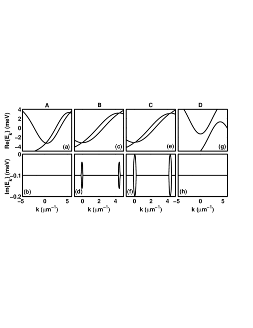
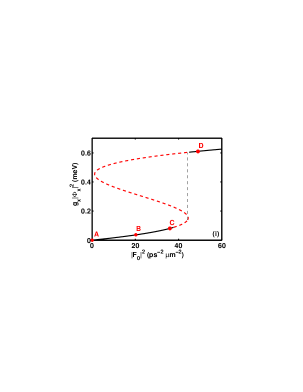
Figure 1: Real (a-g) and imaginary parts (b-h) of the Bogolubov dispersion as a function of the wavevector $k$, for the four regimes A-D marked in panel (i). The exciton interaction energy is $g|\Phi_{x}|^{2}=10^{-4}$ meV (a, b), $g|\Phi_{x}|^{2}=0.04$ meV (c, d), $g|\Phi_{x}|^{2}=0.08$ meV (e, f) and $g|\Phi_{x}|^{2}=0.61$ meV (g, h). (i) Bistable loop in the in-cavity exciton field intensity as a function of the incident pump intensity. The red dashed line represents the unstable solutions. The points labeled with the letters A-D mark the four regimes considered in panels (a-h).

The four operator correlation function describing the correlation of the intensity fluctuations of the in-cavity photon field is defined as usual as:

$$G^{(2)}({\bf r},t;{\bf r^{\prime}},t^{\prime})=\langle\hat{\Psi}_{c}^{\dagger}({\bf r},t)\hat{\Psi}_{c}^{\dagger}({\bf r^{\prime}},t^{\prime})\hat{\Psi}_{c}({\bf r^{\prime}},t^{\prime})\hat{\Psi}_{c}({\bf r},t)\rangle\,.$$ (32)

At the level of the Bogolubov approximation, three- and four-operator averages of the fluctuation field can be neglected and the correlation function (32) can be written in terms of two-operator averages as

$$G^{(2)}({\bf r},{\bf r^{\prime}},t) = |\Phi_{c}({\bf r})|^{2}|\Phi_{c}({\bf r^{\prime}})|^{2}+|\Phi_{c}({\bf r^{\prime}})|^{2}\langle\hat{\psi}_{c}^{\dagger}({\bf r})\hat{\psi}_{c}({\bf r})\rangle$$ (33)

$$+ |\Phi_{c}({\bf r})|^{2}\langle\hat{\psi}_{c}^{\dagger}({\bf r^{\prime}})\hat{\psi}_{c}({\bf r^{\prime}})\rangle$$

$$+ 2\mbox{Re}\{\Phi_{c}({\bf r^{\prime}})^{*}\Phi_{c}({\bf r})\langle\hat{\psi}_{c}^{\dagger}({\bf r},t)\hat{\psi}_{c}({\bf r^{\prime}},0)\rangle\}$$

$$+ 2\mbox{Re}\{\Phi_{c}({\bf r^{\prime}})^{*}\Phi_{c}({\bf r})^{*}\langle\hat{\psi}_{c}({\bf r},t)\hat{\psi}_{c}({\bf r^{\prime}},0)\rangle\}\,.$$

A particularly useful quantity is the reduced correlation function:

$$\bar{G}^{(2)}({\bf r},t;{\bf r^{\prime}},t^{\prime})=\frac{G^{(2)}({\bf r},t;{\bf r^{\prime},t^{\prime}})}{n_{c}({\bf r})\,n_{c}({\bf r^{\prime}})}-1\,,$$ (34)

scaled by the intensity of light

$$n_{c}({\bf r})=|\Phi_{c}({\bf r})|^{2}+\langle\delta\hat{\psi}^{\dagger}_{c}({\bf r})\,\delta\hat{\psi}_{c}({\bf r})\rangle\,,$$ (35)

which can be written in the following simple form:

$$\bar{G}^{(2)}({\bf r},{\bf r^{\prime}},t) \simeq 2\mbox{Re}\left\{\Phi_{c}({\bf r^{\prime}})^{*}\Phi_{c}({\bf r})\langle\hat{\psi}_{c}^{\dagger}({\bf r},t)\hat{\psi}_{c}({\bf r^{\prime}},0)\rangle\right.$$ (36)

$$+ \left.\Phi_{c}({\bf r^{\prime}})^{*}\Phi_{c}({\bf r})^{*}\langle\hat{\psi}_{c}({\bf r},t)\hat{\psi}_{c}({\bf r^{\prime}},0)\rangle\right\}\times$$

$$\times [|\Phi_{c}({\bf r})|^{2}|\Phi_{c}({\bf r^{\prime}})|^{2}]^{-1}\,.$$

In the next section, we will study the spatial and temporal features of this quantity in the most relevant cases.

III 1D uniform system

III.1 Numerical results

In this section we investigate the case of a spatially uniform system under a plane wave monochromatic pump. Spatial homogeneity guarantees that the correlation functions only depend on the relative spatial coordinate $r=x-x^{\prime}$.

We use typical parameters for a GaAs microcavity with $N=10$ quantum wells. In particular, we choose $\hbar\Omega_{R}=10$ meV, $\hbar\gamma_{c}=\hbar\gamma_{x}=\hbar\gamma=0.1$ meV, and we take zero exciton-photon detuning at $k=0$, $E_{x}=\epsilon_{c}(k=0)$. For the sake of simplicity, in the present section we focus our attention on a quasi-one-dimensional geometry where polaritons are transversally confined to a length $l_{1D}\sim 1~{}\mu$m. This corresponds to effective 1D nonlinear coupling constants $g_{x}=1.5\times 10^{-3}$meV $\mu$m and $g_{s}=0.5\times 10^{-3}$ meV $\mu$m. Such geometries are presently under active experimental investigation Dasbach et al. (2005). Extension to the 2D case does not qualitatively affect the physics and will be discussed in Sec. IV in connection to disorder issues.

We consider a configuration where the pump wave vector $k_{p}=2.2~{}\mu$m^-1 is close to the magic wave vector, and the pump energy is $\hbar\omega_{p}-\epsilon_{c}(0)=-8.7$ meV. This configuration allows to study the most significant regimes by simply varying the pump intensity. In Fig. 1 (i), we plot the corresponding exciton field intensity as a function of the pump intensity $|F_{0}|^{2}$: the hysteresis cycle typical of bistable systems is apparent Baas et al. (2004); Carusotto and Ciuti (2004); Ciuti and Carusotto (2005).

In the following, we will consider four different density regimes, marked on the bistability loop by the points A-D. Two of them (A, B) correspond to low-density conditions far from any instability, the point C is very close to the OPO threshold, and point D is in the stable region above the bistability and parametric oscillation region.

In the present uniform system, the elementary excitations on top of the steady-state of the pumped system can be classified in terms of their wavevector $k$. Examples of their Bogolubov dispersion Carusotto and Ciuti (2004) are shown in Fig. 1 (a-h) for the four different regimes marked in Fig. 1 (i) by the points A-D. In the figure, we restrict the field of view to the lower-polariton region that is involved in the physics under investigation here.

For increasing intensities, we observe: i) the low-density parametric regime A (panels a, b), where the Bogolubov modes reduce to the single-particle dispersion; ii) the regime B corresponding to moderate densities (panels c, d), where the imaginary parts are modified and a small region of flattened dispersion appears at the crossing of the Bogolubov modes; iii) the regime C close to OPO threshold (panels e, f), where the imaginary part of one mode tends to zero and a flat region in the Bogolubov dispersion is apparent; iv) the non-parametric configuration D, for intensities larger than the bistability threshold, where the normal and the ghost dispersions are well separated and the eigenmodes of the system tend again to the single-particle dispersion, yet blue-shifted by interactions (panels g, h).

For each of this A-D regimes, we have computed the spatio-temporal pattern of intensity correlations with the model described in the previous section. The results are presented in the next subsections. An analytical interpretation will be given later on in Sec. III.B.

III.1.1 Low-density parametric luminescence

In Fig. 2 (a), we show the spatio-temporal pattern of the intensity correlation in the low-density regime A corresponding to Fig. 1 (a, b): this is characterized by a system of parallel fringes and a butterfly-shaped envelope. The fringe amplitude is almost vanishing inside the cone delimited by the group velocities of the signal and the idler modes (represented by the thin solid lines in the figure) and largest on the edges of the cone. Further away in space and time, it decays back to zero as a consequence of the finite polariton lifetime. At zero delay $t=0$, the central bunching peak around $r=0$ shows a weak narrow dip [Fig.2(b)]. At larger delays [Fig.2(c)], the correlation signal is weaker in between the dot-dashed lines indicating the edges of the cone.

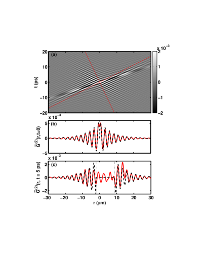
Figure 2: (a) Pattern of the reduced intensity correlations $\bar{G}^{(2)}(r,t)$ as a function of the spatial distance $r$ and of the temporal delay $t$, for the low-density regime A, corresponding to Fig. 1 (a, b). The two thin lines, $r=v_{g}^{s}t$ and $r=v_{g}^{i}t$, highlight the group velocities of the signal and idler modes. (b) Cut of the figure (a) along the zero delay $t=0$ line. (c) Cut along the $t=5$ ps line. In panels (b) and (c), the analytical prediction Eq. (45) is shown as a dashed line. In panel (c), the two vertical dash-dotted lines delimit the region where the analytical result (45) predicts vanishing correlations.

III.1.2 Moderate-density parametric luminescence

In Fig. 3 (a), we show the spatio-temporal pattern in the moderate density regime B corresponding to the energy dispersion shown in Fig. 1 (c, d). As compared to the low-density case, the qualitative shape of the correlation pattern is qualitatively modified: the system of parallel fringes extends in a significant way into the interior of the butterfly shape and the exponential decay in the external region takes place at a slower rate. This latter effect is a direct consequence of the increased lifetime of the Bogolubov modes in the parametric region (see Fig. 1 (d)).

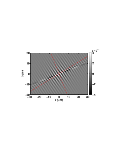
Figure 3: (a) Pattern of the intensity correlations $\bar{G}^{(2)}(r,t)$, for the moderate density regime B, still well below the OPO threshold and corresponding to Fig. 1 (c, d). The two thin lines, $r=v_{g}^{s}t$, and $r=v_{g}^{i}t$, highlight the group velocities of the signal and idler modes.

III.1.3 OPO critical region

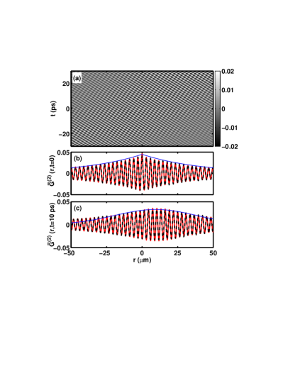
Figure 4: (a) Pattern of the intensity correlations $\bar{G}^{(2)}(r,t)$ for the density regime C just below the OPO threshold and corresponding to Fig. 1 (e, f). (b) Cut of the figure (a) along the zero delay $t=0$ line. (c) Cut along the $t=10$ ps line. In panels (b) and (c), the dashed line is the result of the analytical prediction Eqs. (47) and (LABEL:eq:G2kdom_HD).

In Fig. 4 (a), we show the spatio-temporal pattern for the regime C very close to the OPO threshold. In this case, the system of parallel fringes extends to the whole $(r,t)$ space and correlations are non-vanishing even at very long time and space separations. This is a consequence of the diverging correlation length of fluctuations in the critical region Carusotto and Ciuti (2005). The zero-delay $t=0$ cut of the correlation pattern is shown in Fig. 4 (b) and is characterized by a system of fringes centered at $r=0$ with a central bunching peak. The weak dip that was visible in the weak intensity regime is no longer present.

III.1.4 Non-parametric regime

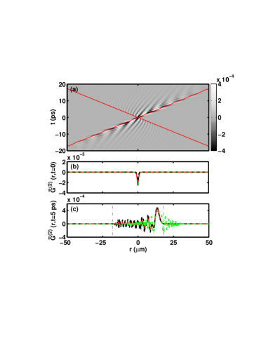
Figure 5: (a) Pattern of the intensity correlations $\bar{G}^{(2)}(r,t)$ for the high-density regime D, corresponding to Fig. 1 (g, h). In this regime, the large blue-shift of the polariton modes prevents the parametric oscillation. The two thin lines $r=\pm v_{g}^{max}t$ mark the maximal group velocities. (b) Cut of the previous figures along the zero delay $t=0$ line. (c) Cut along the $t=5$ ps line. In panels (b) and (c), the analytical prediction Eq. (III.2.3) (red dashed line) and Eq. (III.2.3) (green dash-dotted line) are also shown. In panel (c), the two vertical thin dash-dotted lines delimit the region where both the numerical result and the analytical result (III.2.3) predict vanishing correlations.

For even larger values of the pump intensity beyond the bistability threshold, the system is pushed into an higher density D regime, where the blue-shift induced by interactions brings parametric scattering processes far off-resonance [Fig. 1 (g, h)]. As a consequence, the system of parallel fringes due to parametric correlations almost completely disappears, as it can be seen in Fig. 5 (a). The remaining correlation pattern has an opposite shape, with substantial correlations limited to the region inside the cone delimited by the maximal group velocity of the polariton dispersion. At zero delay $t=0$ [Fig. 5 (b)] no spatial fringe is visible and the only feature is an anti-bunching dip at $r=0$. At finite time delays [Fig. 5 (c)], some spatial fringes appear, but they do not show any dominating periodicity. This suggests that a continuum of processes at different $k$’s are simultaneously taking place, each of them characterized by a different phase velocity.

III.2 Analytic model and interpretation

To physically understand the numerical results presented in the previous section, approximate analytic formulas for the behavior of $\bar{G}^{(2)}$ can be extracted for the most significant limiting cases. To simplify the analysis, we restrict our attention to the lower polariton branch. This approximation is accurate as long as the Rabi splitting is much larger than all other energy scales, e.g. $\hbar\Omega_{R}\gg\gamma$, $\hbar\Omega_{R}\gg g_{x}|\Phi_{x}|^{2},\,g_{s}|\Phi_{c}\,\Phi_{x}|$, and is safely fulfilled in all the cases that we are considering here. In this regime, the dynamics of the system can be described by a single polariton field. Its dispersion, linewidth $\gamma$ and nonlinear interaction coefficient $g$ are immediately obtained from the linear eigenmodes of the Gross-Pitaevskii equations (9) and (II.2) once interactions are neglected Ciuti et al. (2003). At the same level of approximation, also the $k$-dependence of the photon Hopfield factor $C_{k}\simeq C$ can be neglected. As a result, the same Hopfield coefficient $|C|^{4}$ appears in both the numerator and in the denominator of the intensity correlation function (34) of the photon field, which then reduces to the corresponding quantity for the lower-polariton field.

For a spatially homogeneous system under a monochromatic plane wave pump, equations can be written in the momentum space and the reduced second-order correlation function reads

$$\bar{G}^{(2)}({\bf r},t)=G^{(2)}_{1}({\bf r},t)+G^{(2)}_{2}({\bf r},t)=\\ =\frac{2}{|\Phi|^{2}}\,\textrm{Re}\left[\int\!\frac{d^{d}{\bf k}}{(2\pi)^{d}}\,e^{-i({\bf k}-{\bf k}_{p})\cdot{\bf r}}\langle\delta\psi^{\dagger}_{\bf k}(t)\delta\psi_{{\bf k}}(0)\rangle\right]+\\ +\frac{2}{|\Phi|^{4}}\,\textrm{Re}\left[\Phi^{*2}\,\int\!\frac{d^{d}{\bf k}}{(2\pi)^{d}}\,e^{i({\bf k}-{\bf k}_{p})\cdot{\bf r}}\langle\delta\psi_{\bf k}(t)\delta\psi_{\bar{\bf k}}(0)\rangle\right]$$ (37)

where $\bar{{\bf k}}=2{\bf k}_{p}-{\bf k}$. In the presence of quantum fluctuations onlyCiuti et al. (2003); Verger et al. (2007), the normal correlations are

$$\langle\delta\psi^{\dagger}_{\bf k}(t)\delta\psi_{{\bf k}}(0)\rangle=2\pi\hbar^{2}\,\gamma\,g^{2}\,|\Phi|^{4}\int d\omega\frac{e^{i\omega t}}{\Delta_{\bf k}(\omega)}\,,$$ (38)

and the anomalous correlations are

$$\langle\delta\psi_{\bf k}(t)\delta\psi_{\bar{{\bf k}}}(0)\rangle=-2\pi\hbar^{2}\,\gamma\,g\,\Phi^{2}\int d\omega\,e^{-i\omega t}\frac{\tilde{\epsilon}_{\bar{\bf k}}+\hbar\omega+i\frac{\hbar\gamma}{2}}{\Delta_{\bf k}(\omega)}\,.$$ (39)

Here we have introduced the notation $\tilde{\epsilon}_{\bf k}=\epsilon_{\bf k}+2g|\Phi|^{2}-\hbar\omega_{p}$ for the shifted single-particle dispersion of polaritons, ${\bf k}_{p}$ and $\omega_{p}$ respectively indicate the wave vector and the frequency of the pump. The denominator $\Delta_{\bf k}$ is defined in terms of the eigenvalues $E_{\bf k}^{(1,2)}$ of the Bogolubov matrix

$$M_{\bf k}=\left(\begin{array}[]{c c}\tilde{\epsilon}_{\bf k}-i\hbar\gamma/2&g\Phi^{2}\\ -g{\Phi^{*}}^{2}&-\tilde{\epsilon}_{\bar{\bf k}}-i\hbar\gamma/2\end{array}\right)\,,$$ (40)

as

$$\Delta_{\bf k}(\omega)=(\hbar\omega-E_{\bf k}^{(1)})(\hbar\omega-{E_{\bf k}^{(1)}}^{*})(\hbar\omega-E_{\bf k}^{(2)})(\hbar\omega-{E_{\bf k}^{(2)}}^{*})\,.$$ (41)

To better compare to the numerical results, we now restrict our attention to one-dimensional case and we extract analytic formulas for the most significant regimes considered in the previous subsection.

III.2.1 Low-density parametric luminescence

In the low-density limit $|\Phi|\rightarrow 0$ the Bogolubov eigenmodes tend to the single-particle energies with a negligible blue-shift [Fig. 1 (a, b)]. Comparing the expressions (38) and (39) for respectively the normal and the anomalous correlations, it is immediate to see that the former is a factor $g\,|\Phi|^{2}/\hbar\gamma$ smaller and therefore negligible in this limit. By performing the frequency integral in (37) with the method of residuals, the spatial correlation function can be written as

$$\bar{G}^{(2)}(r,t)\simeq-4\pi g\,\textrm{Sgn}(t)\,e^{-\gamma|t|/2}\times\\ \times\textrm{Re}\left\{\int dk\,e^{i(k-k_{p})r}\,\frac{e^{-i\epsilon_{k}t/\hbar}}{\epsilon_{k}+{\epsilon}_{\bar{k}}-2\hbar\omega_{p}-i\hbar\gamma}\right\}\,$$ (42)

In the parametric configuration (see Fig. 1 (a, b)), the dominating contribution to the integral over $k$ is given by the wavevectors around the signal $k_{s}$ and the idler $k_{i}=\bar{k}_{s}=2k_{p}-k_{s}$ modes, where the normal and the ghost dispersions intersect and parametric processes are resonant. We can then approximate the integrand by replacing the energies by their first-order expansions around $k=k_{s,i}$

$$\epsilon_{k}\simeq\epsilon_{k_{s,i}}+\hbar v_{g}^{(s,i)}(k-k_{s,i})\,,$$ (43)

with group velocities

$$v_{g}^{(s,i)}=\frac{1}{\hbar}\,\partial_{k}\epsilon(k)|_{k_{s,i}}\,.$$ (44)

In this way, we obtain

$$\bar{G}^{(2)}_{2}(r,t)\simeq 8\pi^{2}\frac{g}{\hbar\Delta v_{g}}\mbox{Sgn}(t)e^{-\gamma|t|/2}S\sin(Kr-\Omega t)\times\\ \times[\theta(tSR_{s})e^{-\kappa R_{s}}-\theta(-tSR_{i}(r,t))e^{\kappa R_{i}(r,t)}]\,,$$ (45)

where $S=\mbox{Sgn}(\Delta v_{g})$ and $\Delta v_{g}=v_{g}^{(s)}-v_{g}^{(i)}$.

From this expression, it is immediate to see that the system of parallel fringes has a frequency $\hbar\Omega={\epsilon}_{k_{s}}-\hbar\omega_{p}$ and a wavevector $K=k_{s}-k_{p}$ determined by the interference of the signal/idler and the pump mode. The analytic form of the zero delay $t=0$ fringe pattern resulting from the combination of $\sin$ and $\theta$ functions is responsible for the dip at $r=0$ that is visible in Fig.2(b). The temporal decay of the correlation occurs on the same time scale as the bare polariton decay rate $\gamma$. The spatial decay away from the butterfly edges (we have set $R_{s,i}(r,t)=r-v_{g}^{(s,i)}t$) occurs on a length scale $\kappa^{-1}=|\Delta v_{g}|\,/\gamma$.

Furthermore, the analytical formula (45) shows that no correlation is present inside the cone marked by the thin lines in the Fig. 2 and defined (for $t>0$) by the condition $R_{s}<0$ and $R_{i}>0$ (for $t<0$ the signs are exchanged). The physics behind this fact is illustrated by the simple geometric construction shown in Fig. 6: pairs of entangled signal/idler polaritons are generated at all times and positions by the parametric conversion of quantum fluctuations into real excitations. Signal and idler polaritons then propagate with group velocities respectively $v_{g}^{s,i}$ and transport the correlation to distant pairs of points. It is easy to see that the shaded region inside the cone can never be reached by such a process. An analogous reasoning was used in Ref. Carusotto et al. (2008) to explain the correlation signal observed in numerical calculations of Hawking radiation from acoustic black holes. As polaritons decay at a rate $\gamma$, the same construction shows that the correlation signal has to decay in space with the characteristic length $\kappa^{-1}=\Delta v_{g}/\gamma$.

Figure 6: Geometric construction to determine the pairs of points in space-time that are correlated in the low-density parametric luminescence regime. The shaded area highlights the region of space-time which is not correlated with the point ($r=0$, $t=0$). The point ($r=0$, $t=0$) is parametrically correlated with the point $\alpha$, as a result of the parametric emission event occurring at the point marked with a star. The same holds for the point $\beta$. Solid lines mark the motion of signal (blue) and idler (red) particles. No parametric event can instead produce correlations between the point ($r=0$, $t=0$) and the point $\delta$ located inside the shaded region.

The perfect agreement between this analytic approximation and the numerical result is highlighted in Fig. 2 (b, c). The lower polariton parameters $g$, $\gamma$, $\epsilon_{k}$ are calculated from the linear eigenmodes of the GP equations (9) and (II.2). As expected for a Bogolubov theory Castin (2001), for a given blue shift $g\,|\Phi|^{2}$ the rescaled correlation function is proportional to the nonlinear coupling constant $g$.

Before proceeding, it is interesting to note that for a pump at normal incidence $k_{p}=0$, one has $k_{s}=-k_{i}$ and a vanishing relative frequency $\Omega=0$. The spatial fringes are then independent on time. From an experimental point of view, this configuration appears to be the most suitable one to observe the predicted features as it is less subject to the finite time resolution of photodetectors.

III.2.2 OPO critical region

For pump intensities just below the OPO threshold, $g|\Phi|^{2}\lesssim g|\Phi_{OPO}|^{2}=\hbar\gamma/2$, the Bogolubov spectrum strongly differs from the single-particle one [Fig. 1 (e, f)]. In particular, the imaginary part of one of the two eigenvalues tends to zero in the vicinity  of $k=k_{s}$ and $k=k_{i}=2k_{p}-k_{s}$. In this case, it is easy to see that for wavevectors in the vicinity of $k_{s,i}$ one has $\textrm{Re}[E_{k_{s,i}+k}^{(1)}]=\textrm{Re}[E_{k_{s,i}+k}^{(2)}]$ and $\textrm{Re}[E_{k_{i}-k}^{(1)}]=-\textrm{Re}[E_{k_{s}+k}^{(1)}]$. In this region, the eigenvalues can be approximated with the expression

$${E_{k}^{(1,2)}}_{\overrightarrow{k\rightarrow k_{s,i}}}\pm E_{0}+\hbar V_{g}(k-k_{s,i})-\frac{i\hbar}{2}[\gamma\mp\gamma_{0}\pm\gamma_{1}(k-k_{s,i})^{2}]\,,$$ (46)

where $V_{g}=\partial_{k}E_{k}|_{k_{s}}/\hbar=\partial_{k}E_{k}|_{k_{i}}/\hbar$ and $\hbar\gamma_{0}=2g\,|\Phi|^{2}\lesssim\hbar\gamma$, the equality holding exactly at threshold $|\Phi|^{2}=|\Phi_{OPO}|^{2}$. Following the procedure already adopted in the previous subsection, we perform the frequency integration in (39) with the method of residuals and we expand the function in $k$ around $k_{s,i}$. Then, by retaining only the dominant contribution (which, as expected, diverges exactly at threshold $\gamma=\gamma_{0}$) and using the relations (46), we finally obtain the expressions

$$\bar{G}^{(2)}_{1}(r,t) \simeq \frac{2g}{\hbar}e^{-(\gamma-\gamma_{0})|t|/2}\,\cos(Kr-\frac{E_{0}t}{\hbar})\times$$ (47)

$$\times \int dk\,\frac{\cos(kR)\,e^{-\gamma_{1}k^{2}|t|/2}}{\gamma-\gamma_{0}+\gamma_{1}k^{2}}\,,$$

and

$$\bar{G}^{(2)}_{2}(r,t) \simeq -\frac{4\pi g}{\hbar^{2}\gamma_{0}}e^{-(\gamma-\gamma_{0})|t|/2}\times$$

$$\times \mbox{Re}\left\{\int dk\,\frac{e^{ikR-\gamma_{1}k^{2}|t|/2}}{\gamma-\gamma_{0}+\gamma_{1}k^{2}}\right.\times$$

$$\times \left[(\bar{E}_{s}+\Delta V_{g}^{(s)}k+i\hbar\gamma_{0}/2)\,e^{-iKr+iE_{0}t/\hbar}\right.+$$

$$+ \left.\left.(\bar{E}_{i}+\Delta V_{g}^{(i)}k+i\hbar\gamma_{0}/2)\,e^{iKr-iE_{0}t/\hbar}\right]\right\}\,,$$

with $R=r-V_{g}t$, $\bar{E}_{s,i}=\tilde{\epsilon}_{k_{s,i}}\mp E_{0}$, $K=k_{s}-k_{p}$, and $\Delta V_{g}^{(s,i)}=V_{g}-v_{g}^{(s,i)}$.

This result can be further simplified by introducing the approximations $\bar{E}_{s}\simeq\bar{E}_{i}\simeq 0$ and $\Delta V_{g}^{(s)}\simeq\Delta V_{g}^{(i)}\simeq 0$. In this case, the anomalous correlation disappears

$$\bar{G}^{(2)}_{2}(r,t) \simeq \frac{4\pi g}{\hbar}e^{-(\gamma-\gamma_{0})|t|/2}\cos(Kr-E_{0}t/\hbar)\times$$ (49)

$$\times \int dk\sin(kR)\frac{e^{-\gamma_{1}k^{2}|t|/2}}{\gamma-\gamma_{0}+\gamma_{1}k^{2}}=0\,,$$

as the integrand is odd in $k$, and the spatial correlations are dominated by the normal contribution $\bar{G}^{(2)}\simeq\bar{G}^{(2)}_{1}$. The explicit expression of $\bar{G}^{(2)}_{1}$ is given in (47): the Fourier transform of the product of a Gaussian and a Lorentzian function corresponds, in real space, to the convolution of an exponential and a gaussian function.

At zero delay $t=0$ [Fig. 4 (b)], the Gaussian reduces to a delta-function in space and the correlation signal shows an exponential decay in space with a characteristic length

$$\ell\simeq\sqrt{\frac{\gamma_{1}}{\gamma-\gamma_{0}}}.$$ (50)

As expected on the basis of general arguments on phase transition, and previously observed in Monte Carlo simulations Carusotto and Ciuti (2005), the characteristic length $\ell$ diverges as the OPO threshold is approached $\gamma_{0}\rightarrow\gamma$. In contrast to the expression (45) for the weak intensity case, the zero delay $t=0$ fringe pattern now has a $\cos$ form with a simple bunching peak at $r=0$.

At longer times, the spatial width of the Gaussian grows as $\sqrt{t}$, so that for short to intermediate distances, the dependence is dominated by the Gaussian factor. This effect is clearly visible in Fig. 4 (c). The overall exponential decay in time occurs on a characteristic time

$$\tau\simeq\frac{1}{\gamma-\gamma_{0}}.$$ (51)

which again diverges as the critical point is approached.

III.2.3 Non-parametric regime

The non-parametric regime shown in Fig. 1 (g,h) corresponds to the case where the polariton and ghost branches do not intersect, i.e. $\tilde{\epsilon}_{k}+\tilde{\epsilon}_{\bar{k}}\neq 0$ for all $k$. This regime is generally realized when the frequency of the pump is very much red-detuned with respect to the renormalized polariton dispersion and, in our configuration, is fulfilled for pump intensities above the bistability loop.

In this regime, the Bogolubov eigenmodes can be approximated by the single particle dispersion blue-shifted by the interaction, i.e. $E_{k}\simeq\tilde{\epsilon}_{k}-i\hbar\gamma/2$ and an equation formally equivalent to (42) still holds. However, since the denominator remains finite for all $k$, no pole can be identified. However, the region of the polariton dispersion that minimizes the denominator gives the dominant contribution. In the case of Fig. 1 (g), this happens at $k=k_{p}$. It is therefore convenient to expand the energy dispersion at second order in $k-k_{p}$. Performing this approximation in the denominator, we obtain the following formula for the correlation function:

$$\bar{G}^{(2)}(r,t) \simeq 4g(\pi\frac{g|\Phi|^{2}}{\tilde{\epsilon}_{k_{p}}}-2)e^{-\gamma|t|/2}\times$$

$$\times \mbox{Re}\left\{\int dk\,e^{-ikr}\frac{e^{i\tilde{\epsilon}_{k+k_{p}}t/\hbar}}{2\tilde{\epsilon}_{k_{p}}+2u_{p}k^{2}+i\mbox{Sgn}(t)\hbar\gamma}\right\}\,.$$

To further simplify this expression, we can expand also the energy exponents, which leads to

$$\bar{G}^{(2)}(r,t) \simeq 4g(\pi\frac{g|\Phi|^{2}}{\tilde{\epsilon}_{k_{p}}}-2)e^{-\gamma|t|/2}\mbox{Re}\left\{e^{i\tilde{\epsilon}_{k_{p}}t/\hbar}\times\right.$$

$$\times \left.\int dke^{-ikR}\frac{e^{iu_{p}k^{2}t/\hbar}}{2\tilde{\epsilon}_{k_{p}}+2u_{p}k^{2}+i\mbox{Sgn(t)}\hbar\gamma}\right\}\,.$$

Here, we have set $R=r-v_{g}^{(p)}t$, $v_{g}^{(p)}=\partial_{k}\tilde{\epsilon}_{k}|_{k_{p}}/\hbar$ and $u_{p}=\partial^{2}_{k}\tilde{\epsilon}|_{k_{p}}/2$.

The integral over $k$ is of the Fresnel kind and describes the interference produced at the point $(R,t)$ by the different $k$-modes with a gapped and quadratic dispersion. For zero time delay $t=0$, the correlations have a typical anti-bunching character: they are everywhere negative and are strongest at $r=0$. Further away, they monotonically tend to zero with an exponential law of characteristic length $\kappa^{-1}=\sqrt{u_{p}/\tilde{\epsilon}_{k_{p}}}$ determined by the gap between the renormalized polariton and ghost branches .

The most apparent deviation between the analytical form (III.2.3) and the numerical result shown Fig.5(c) consists of a tail in the analytic approximation that extends up to large distances. This has a simple interpretation: the quadratic approximation of the dispersion eliminates all bounds in the group velocity and predicts correlations at any distances. In contrast, the correct dispersion has an upper bound $v_{g}^{max}$ to the group velocity, which restricts the possible correlations to the $|r|<v_{g}^{max}\,|t|$ region marked by the thin lines in Fig. 5(a) and (c): this intepretation is confirmed by the much better agreement of the (III.2.3) prediction where the group velocity is correctly taken into account.

IV Two-dimensional and disordered system

In this final section we apply our model to the more general case of a two dimensional inhomogeneous system. In particular, we wish to investigate how the conclusions of the previous sections are affected by the presence of exciton and photon disorder.

Realistic system parameters for a GaAs microcavity with $N=2$ quantum wells are used, with $\hbar\Omega_{R}=3.5$ meV, $\hbar\gamma_{c}=\hbar\gamma_{x}=\hbar\gamma=0.2$ meV, zero exciton-photon detuning. For the nonlinear interaction constant we take $g_{x}=1.5\times 10^{-3}$ meV $\mu$m² and $g_{s}=0.5\times 10^{-3}$ meV $\mu$m². We consider a configuration where the pump is orthogonal to the cavity plane, $k_{p}=0$ and we take $\hbar\omega_{p}-\epsilon_{c}(0)=-3$ meV. This orthogonal pump configuration is the most suitable one in view of experiments, as it is least affected by the temporal resolution of the photon detectors.

The correlation pattern for different values of the pump intensity, corresponding to the low-density limit, the critical OPO region and the non-parametric configuration are shown in Fig. 7 (a, b, c) for a two dimensional system in the absence of disorder. All the features discussed in the previous section for the 1D case are still apparent. In particular, in the low-density case, the correlations disappear for distances smaller that $|r_{max}(t)|=v_{g}t$, $\pm v_{g}$ being the group velocities of polaritons in the signal and idler modes, and they decay exponentially. On the other hand, in the vicinity of the OPO threshold, correlations extend everywhere. In the non-parametric configuration, correlations are non vanishing only for distances smaller than $r=v_{g}^{max}t$, $v_{g}^{max}$ being the largest group velocity.

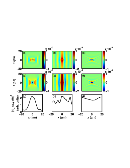
Figure 7: Intensity correlation pattern $\bar{G}^{(2)}({\bf r},t)$ as a function of the spatial coordinate $x$ and of the temporal delay $t$ along a $y=0$ line for a 2D system. Panels (a-c) are for a uniform case, while panels (d-f) are for a disordered system. The pump intensity is varied from a low value (a, d), to a value close to the OPO threshold (b, e) and to a value well above the bistability loop (c, f) where parametric processes are forbidden. Panels (g-i) show the coherent photon field profiles $|\Phi_{c}(r)|^{2}$ corresponding to the disordered case of panels (d-f).

We assume white noise disorder for the exciton field of amplitude $2$ meV and a gaussian-correlated disorder for the photon field, with amplitude $U_{dis}^{c}=0.5$ meV and a correlation length of $\xi_{c}=7~{}\mu$m. The results of the numerical calculations are summarized in Fig. 7 (d-i): the profile of the coherent photon field $|\Phi_{c}({\bf r})|^{2}$ in the three cases is shown in panels (g-i) and the corresponding spatio-temporal patterns of correlations are shown in panel (d-f). The realization of the disorder potential is the same for the three values of the pump intensity.

Even if it is responsible for large density modulations, the considered disorder is never able to destroy the near-field correlation pattern. Of course the pattern would eventually disappear if a much stronger disorder was considered, that is able to fragment the coherent field in disconnected parts. However, this latter situation is quite unusual for state-of-the-art GaAs microcavities.

From the comparison with the corresponding correlation patterns for a clean system [Fig. 7 (a-c)], we can still appreciate a slight modification in the pattern. Disorder is responsible for these modifications via three main effects: i) the exciton and photon resonances are broadened; ii) ${\bf k}$-conservation is broken, which softens the condition for parametric processes; iii) the group velocity is no longer a well defined concept, so the contour of the butterfly shape in Fig. 7 (d) is smeared out with respect to panel (a).

V Conclusions

We have developed a formalism to compute the second order spatial correlation function of polaritons in a planar microcavity. This quantity directly transfer into the near-field intensity correlations of the emitted light.

We have computed the spatio-temporal pattern of correlations in different pumping regimes, ranging from the parametric luminescence regime, to the critical region just below the parametric oscillation threshold, and to the strong pumping regime where a large blue-shift of the polariton modes is able to prevent parametric oscillation.

For each regime, we have identified the key features of the correlation pattern. In the uniform case, we have compared our results to the predictions of approximate analytic models which provide a physical interpretation to the observed patterns. An orthogonal pump geometry appears as the optimal choice for the experimental observation as it reduces the required temporal resolution of photo-detectors. We have verified that the correlation patterns are not qualitatively modified by a realistic disorder as long as the coherent polaritons remain delocalized in space.

The conclusions of the present work confirm the expectation that intensity correlations can be a very powerful tool to study the dynamics of quantum fields in condensed matter systems. A study of more complex geometries is presently under way.

VI Acknowledgements

We are grateful to Cristiano Ciuti for continuous stimulating discussions. D. S. acknowledges the financial support from the Swiss National Foundation (SNF) through the fellowship number PBELP2-125476.

VII Appendix

In this Appendix, we discuss the connection between the photon field inside the cavity and the emitted light. In particular, we show that the calculated in-cavity intensity correlations directly transfer to the near-field correlations of the emitted light.

We consider a planar cavity along the $x-y$ plane with a quantum well placed at $z=0$ and mirrors whose external surface is at $z=\pm z_{m}$. In Fourier space, the external field $E_{out}({\bf k},\omega)$, resulting from the transmission across the mirror is related to the in-cavity field $E_{in}({\bf k},\omega)$ at the quantum well position via the complex transmission coefficient $\tau({\bf k},\omega)=T^{1/2}e^{i\phi({\bf k},\omega)}$:

$$E_{out}({\bf r},z,t)=\int\frac{d^{2}{\bf k}}{(2\pi)^{2}}\int\frac{d\omega}{2\pi}e^{i({\bf k}\cdot{\bf r}-\omega t)}e^{ik_{z}(k)(z-z_{m})}\times\\ \times\tau({\bf k},\omega)E_{in}({\bf k},\omega)\,.$$ (54)

For simplicity, we have neglected here the ${\bf k}$- and $\omega$-dependence of the transmittivity $T$ as we are resticting to frequencies well within the stop band of the mirror where $T$ is almost constant (see Fig.8(a)).

For frequencies close to the $\mathbf{k}=0$ cavity frequency $\omega_{0}$ and at low wave vectors $\mathbf{k}$, the phase of the transmission coefficient can be accurately approximated by the expansion

$$\phi({\bf k},\omega)=\phi(0,\omega_{0})+\Delta_{t}(\omega-\omega_{0})-\frac{c}{2\omega_{0}}\Delta_{z}k^{2}\,,$$ (55)

with

$$\Delta_{t}=\left.\frac{\partial\phi}{\partial\omega}\right|_{\omega_{0}}\,$$ (56)

and

$$\Delta_{z}=\frac{\omega_{0}}{c}\left.\frac{\partial^{2}\phi}{\partial k^{2}}\right|\,.$$ (57)

The transmitted field thus reduces to

$$E_{out}({\bf r},z,t)\simeq\mathcal{B}\,\int\frac{d^{2}{\bf k}}{(2\pi)^{2}}e^{i{\bf k}\cdot{\bf r}}e^{-i\frac{c}{2\omega_{0}}(z-\Delta_{z})k^{2}}E_{in}({\bf k},t-\Delta_{t})\,,$$ (58)

where we have used the relation (valid in the air)

$$k_{z}(k)=\sqrt{\omega_{0}^{2}/c^{2}-k^{2}}\simeq\omega_{0}/c-c/2\omega_{0}k^{2}\,,$$ (59)

and we have included the transmittivity $T$ and a global phase into the multiplicative constant ${\mathcal{B}}$.

Without the mirror, the field $E_{out}({\bf r},z,t)$ would be given by

$$E_{out}({\bf r},z,t)\simeq\int\frac{d^{2}{\bf k}}{(2\pi)^{2}}e^{i{\bf k}\cdot{\bf r}}e^{-i\frac{c}{2\omega_{0}}zk^{2}}E_{in}({\bf k},t)\,.$$ (60)

Comparison between Eqs. (58) and (60) shows that the only effect of the mirror on the external field is to give a time shift of $\Delta_{t}$ and a longitudinal space shift $\Delta_{z}$.

We now demonstrate that the expansion (55) holds for a typical high-quality GaAs microcavity with $N$ DBR’s mirrors Deveaud (2005). To this purpose, we employ the standard transfer matrix approach savona_ssc to compute the ${\bf k}$- and $\omega$-dependent complex transmission coefficient $\tau(\omega,{\bf k})$ across the top mirror placed between the cavity and the air. We consider the typical case where the DBR’s mirrors are composed by two alternate dielectric layers with index of refraction $n_{1}$ and $n_{2}$ and length $l_{1}$ and $l_{2}$, respectively, such as $l_{1}/n_{1}\simeq l_{2}/n_{2}\simeq\lambda_{0}/4$, $\lambda_{0}=2\pi c/\omega_{0}$ being the cavity wavelength. The transfer matrix for the transmission from the cavity to the air is savona_ssc

$$M=T_{a2}T_{21}^{-1}M_{12}^{N}T_{1c}\,,$$ (61)

where $T_{a2}$, $T_{12}$ and $T_{1c}$ are the matrices describing the transmission across the interfaces between the air and the dielectric $2$, between the dielectric $1$ and the dielectric $2$ and between the dielectric $1$ and the cavity, while

$$M_{12}=T_{21}M_{2}T_{12}M_{1}\,,$$ (62)

is the transfer matrix describing the transmission across the periodic block formed by the two dielectric layers. Since

$$M\left(\begin{array}[]{c}1\\ \rho\end{array}\right)=\left(\begin{array}[]{c}\tau\\ 0\end{array}\right)$$ (63)

the transmission coefficient is given by

$$\tau=\frac{\mbox{det}(M)}{M_{22}}\,.$$ (64)

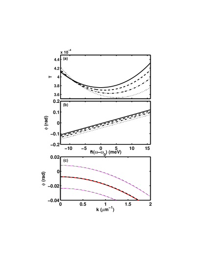
Figure 8: Transmittivity (a) and transmission phase (b) across the $\lambda/4$ DBR mirror between cavity and air as a function of the frequency $\omega$, for a given wavevector $k=0$ (solid line), $k=1~{}\mu$m^-1 (dashed), $k=1.5~{}\mu$m^-1 (dot-dashed) and $k=2~{}\mu$m^-1 (dotted). Parameters are $l_{1}=65$ nm, $l_{2}=75$ nm, $n_{1}=3$, $n_{2}$=3.5, $n_{c}=3.4$, $L_{c}=290$ nm and $N=22$. The cavity frequency $\omega_{0}=\pi c/n_{c}L_{c}$ is located at the center of the mirror stop band. (c) Transmission phase across the same DBR mirror as a function of the wavevector $k$, for a give frequency $\omega-\omega_{0}=0$ (thick solid line) and $\hbar(\omega-\omega_{0})=\pm 2$ meV (thin lines). Dashed lines are obtained by fitting the numerical results with Eq. (55), which gives $\Delta_{z}\simeq 140$ nm.

Examples summarized in Fig. 8. In panel (a), we show the frequency dependent transmission amplitude $T$, for in-plane wave vectors ranging from $k=0$ and $k=2~{}\mu$m^-1. The relative variation is less than 10% in the interval of frequencies and wave vectors considered which validates the assumption underlying (). In panel (b) we display the phase of the transmission coefficient as a function of the frequency. For all values of the in-plane wavevector $k$, the linear dependence assumed in Eq. (55) is accurately verified with the same $\Delta_{t}\simeq 5$ fs. This result confirms the validity of the expansion (55). In panel (c), we show the dependence of the phase $\phi$ on the wavevector $k$, for different values of the frequency $\hbar\omega=-2,0,2$ meV. Again the dependence assumed in Eq. (55) is verified with the same value of $\Delta_{z}\sim 140$ nm.

It is important to note that this small spatial shift $\Delta_{z}$ does not scale with the number $N$ of layers in the DBR mirror, as it could be intuitively supposed. This result originates from the fact that within the stop band the transfer matrix $M_{12}$ (and consequently $M_{12}^{N}$) has real eigenvalues, and thus does not induce any extensive phase shift.

The results of this appendix show that the only effect of the mirror on the near-field correlation pattern is the following: the light detected outside of the cavity appears to be generated at a slightly earlier time and at a slightly displaced longitudinal position as compared to the quantum well position. In the experiments one has therefore simply to focus the optical detection on this shifted position.

References

- Pitaevskii and Stringari (2003) L. Pitaevskii and S. Stringari, Bose-Einstein condensation (Oxford, 2003).
- Bloch et al. (2008) I. Bloch, J. Dalibard, and W. Zwerger, Rev. Mod. Phys. 80, 885 (2008).
- Lugiato et al. (1998) L. A. Lugiato, M. Brambilla, and A. Gatti, Adv. At. Mol. Opt. Phys. 40, 229 (1998).
- Gatti et al. (2009) A. Gatti, E. Brambilla, L. Caspani, O. Jedrkiewicz, and L. A. Lugiato, Phys. Rev. Lett. 102, 223601 (2009).
- Zambrini et al. (2000) R. Zambrini, M. Hoyuelos, A. Gatti, P. Colet, L. Lugiato, and M. San Miguel, Phys. Rev. A 62, 063801 (2000).
- Lopez et al. (2008) L. Lopez, N. Treps, B. Chalopin, C. Fabre, and A. Maître, Phys. Rev. Lett. 100, 013604 (2008).
- Delaubert et al. (2008) V. Delaubert, N. Treps, C. Fabre, H. A. Bachor, and P. Refregier, EPL 81, 44001 (2008).
- Balbinot et al. (2008) R. Balbinot, A. Fabbri, S. Fagnocchi, A. Recati, and I. Carusotto, Phys. Rev. A 78, 021603(R) (2008).
- Carusotto et al. (2008) I. Carusotto, S. Fagnocchi, A. Recati, R. Balbinot, and A. Fabbri, New J. Phys. 10, 103001 (2008).
- Carusotto et al. (2009) I. Carusotto, R. Balbinot, A. Fabbri, and A. Recati, Eur. Phys. J. D , DOI: 10.1140/epjd/e2009-00314-3(2009).
- Butcher and Cotter (1993) P. N. Butcher and D. Cotter, The elements of nonlinear optics (Cambridge University Press, Cambridge, 1993).
- Walls and Milburn (1994) D. F. Walls and G. J. Milburn, Quantum Optics (Springer, Berlin, 1994).
- Savvidis et al. (2000) P. G. Savvidis, J. J. Baumberg, R. M. Stevenson, M. S. Skolnick, D. M. Whittaker, and J. S. Roberts, Phys. Rev. Lett. 84, 1547 (2000); R. M. Stevenson, V. N. Astratov, M. S. Skolnick, D. M. Whittaker, M. Emam-Ismail, A. I. Tartakovskii, P. G. Savvidis, J. J. Baumberg, and J. S. Roberts, Phys. Rev. Lett. 85, 3680 (2000); R. Houdré, C. Weisbuch, R. P. Stanley, U. Oesterle, and M. Ilegems, Phys. Rev. B 61, R13333 (2000).
- Ciuti et al. (2003) C. Ciuti, P. Schwendimann, and A. Quattropani, Semicond. Sci. Technol. 18, S279 (2003).
- Carusotto and Ciuti (2005) I. Carusotto and C. Ciuti, Physical Review B 72, 125335 (2005).
- Drummond and Dechoum (2005) P. D. Drummond and K. Dechoum, Phys. Rev. Lett. 95, 083601 (2005).
- Deveaud (2005) B. Deveaud (Ed.), Special Issue: Physics of Semiconductor Microcavities, phys. stat. sol. (b) 242, 2145-2356 (2005).
- Savasta et al. (2005) S. Savasta, O. DiStefano, V. Savona, and W. Langbein, Phys. Rev. Lett. 94, 246401 (2005).
- Romanelli et al. (2007) M. Romanelli, C. Leyder, J. P. Karr, E. Giacobino, and A. Bramati, Phys. Rev. Lett. 98, 106401 (2007).
- Baas et al. (2006) A. Baas, J.-P. Karr, M. Romanelli, A. Bramati, and E. Giacobino, Phys. Rev. Lett. 96, 176401 (2006).
- Marino (2008) F. Marino, Phys. Rev. A 78, 063804 (2008).
- Verger et al. (2007) A. Verger, I. Carusotto, and C. Ciuti, Phys. Rev. B 76, 115324 (2007).
- Sarchi et al. (2009) D. Sarchi, M. Wouters, and V. Savona, Phys. Rev. B 79, 165315 (2009).
- Castin (2001) Y. Castin, in Coherent atomic matter waves, edited by R. Kaiser, C. Westbrook, and F. David (EDP Sciences and Springer-Verlag, 2001), Lecture Notes of Les Houches Summer School, p. 1. ArXiv:cond-mat/0105058.
- Carusotto and Ciuti (2004) I. Carusotto and C. Ciuti, Phys. Rev. Lett. 93, 166401 (2004).
- Rochat et al. (2000) G. Rochat, C. Ciuti, V. Savona, C. Piermarocchi, A. Quattropani, and P. Schwendimann, Phys. Rev. B 61, 13856 (2000).
- Ben-Tabou de Leon and Laikhtman (2001) S. B. de-Leon and B. Laikhtman, Phys. Rev. B 63, 125306 (2001).
- Castin and Dum (1997) Y. Castin and R. Dum, Phys. Rev. Lett. 79, 3553 (1997).
- Ciuti and Carusotto (2006) C. Ciuti and I. Carusotto, Phys. Rev. A 74, 033811 (2006).
- De Liberato, Ciuti, and Carusotto (2007) S. De Liberato, C. Ciuti, and I. Carusotto, Phys. Rev. Lett. 98, 103602 (2007).
- De Liberato, Gerace, Ciuti, and Carusotto (2009) S. De Liberato, D. Gerace, I. Carusotto, and C. Ciuti, Phys. Rev. A 80, 053810 (2009).
- Dasbach et al. (2005) G. Dasbach, C. Diederichs, J. Tignon, C. Ciuti, P. Roussignol, C. Delalande, M. Bayer, and A. Forchel, Phys. Rev. B 71, 161308(R) (2005).
- Baas et al. (2004) A. Baas, J. P. Karr, H. Eleuch, and E. Giacobino, Phys. Rev. A 69, 023809 (2004).
- Ciuti and Carusotto (2005) C. Ciuti and I. Carusotto, Phys. Stat. Sol. (b) 242, 2224 (2005).
- (35) V. Savona, L. C. Andreani, P. Schwendimann, A. Quattropani, Solid State Comm., 93, 733 (1995).