Static wormholes on the brane inspired by Kaluza-Klein gravity

Abstract

We use static solutions of $5$-dimensional Kaluza-Klein gravity to generate several classes of static, spherically symmetric spacetimes which are analytic solutions to the equation ${}^{(4)}R=0$, where ${}^{(4)}R$ is the four-dimensional Ricci scalar. In the Randall $\&$ Sundrum scenario they can be interpreted as vacuum solutions on the brane. The solutions contain the Schwarzschild black hole, and generate new families of traversable Lorenzian wormholes as well as nakedly singular spacetimes. They generalize a number of previously known solutions in the literature, e.g., the temporal and spatial Schwarzschild solutions of braneworld theory as well as the class of self-dual Lorenzian wormholes. A major departure of our solutions from Lorenzian wormholes a la Morris and Thorne is that, for certain values of the parameters of the solutions, they contain three spherical surfaces (instead of one) which are extremal and have finite area. Two of them have the same size, meet the “flare-out” requirements, and show the typical violation of the energy conditions that characterizes a wormhole throat. The other extremal sphere is “flaring-in” in the sense that its sectional area is a local maximum and the weak, null and dominant energy conditions are satisfied in its neighborhood. After bouncing back at this second surface a traveler crosses into another space which is the double of the one she/he started in. Another interesting feature is that the size of the throat can be less than the Schwarzschild radius $2M$, which no longer defines the horizon, i.e., to a distant observer a particle or light falling down crosses the Schwarzschild radius in a finite time.

PACS: 04.50.+h; 04.20.Cv

Keywords: Wormholes; Braneworld; General Relativity; Exact Solutions.

1 Introduction

The idea that remote parts of the universe, or even that different universes, could be connected by smooth bridges or tunnels constitutes a very intriguing concept, which for many decades has captivated the imagination of science fiction lovers [1], [2]. In physics, spacetimes containing such bridges (called “wormholes” by J.A. Wheeler) appear in general relativity as solutions of the Einstein field equations. Nearly half a century ago, the concept of wormholes lead Wheeler to the discussion of topological entities called geons [3] and to the conception of geometrodynamics [4], where “matter comes from no matter”, and “charge comes from no charge”.

Lately, after the fundamental papers by Morris, Thorne and Yurtsewer [5] and Morris and Thorne [6], the notion of traversable Lorentzian wormholes has gained much attention within the physics community. These authors showed that such wormholes could, in principle, allow humans not only to travel between universes, or distant parts of a single universe, but also to construct time machines. It has been suggested that black holes and wormholes are interconvertible. In particular that stationary wormholes could be possible final states of black-hole evaporation [7]. Also, that astrophysical accretion of ordinary matter could convert wormholes into black holes [8] (this issue has recently been discussed in literature and different approaches give, in general, different results - see [9], [10]).

Today, it is well known that a wormhole geometry can only appear as a solution of the Einstein field equations if the energy-momentum tensor (EMT) of the matter supporting such a geometry violates the null energy condition (NEC) at least in the neighborhood of the wormhole throat [11]-[13] (matter that violates the NEC is usually called exotic). Although in general relativity there are many examples of matter that are consistent with wormhole spacetimes (see, e.g., [14]-[16]), none of them are observable in the real world of astrophysics: “all these spacetimes still remain in the domain of fiction” [19]. This is a very important and challenging issue in wormhole physics, which is known as the “exotic matter problem”. There are numerous attempts at solving this issue in the literature. Some consider alternative theories of gravity [20]-[22] or invoke quantum effects in curved spacetimes, considering wormholes as semiclasical objects [23], [24]. Recently, a general no-go theorem was proved by Bronnikov and Starobinsky showing the absence of wormholes in scalar-tensor gravity without ghosts [25].

A different approach to this issue arises in the context of higher-dimensional theories. In Kaluza-Klein gravity the exotic matter necessary for the formation of a wormhole can appear from the off-diagonal elements of the metric (the gauge fields) and from the $\gamma_{55}$ component of the metric (the scalar field), rather than coming from some externally given exotic matter [26]. Also the so-called Einstein-Gauss-Bonnet theory admits wormhole solutions that would not violate the NEC provided the Gauss-Bonnet coupling constant is negative [27], [28]. In addition, it has been proposed that braneworld gravity provides a natural scenario for the existence of traversable wormholes [29], [30]. This is because the local high-energy effects and non-local corrections from the Weyl curvature in the bulk could lead to an effective violation of the NEC on the brane even when the standard-model fields satisfy the energy conditions. In this paper we adhere to the latter framework and develop a number of spherically symmetric, static Lorentzian wormholes which are analytic solutions to the equations on the brane.

In the Randall $\&$ Sundrum braneworld scenario [31] the effective equations for gravity in $4D$ were derived by Shiromizu, Maeda and Sasaki [32]. In vacuum, when matter on the brane is absent and the $4$-dimensional cosmological constant vanishes, these equations reduce to

$$^{(4)}G_{\alpha\beta}=-\epsilon E_{\alpha\beta},$$ (1)

where ${}^{(4)}G_{\alpha\beta}$ is the usual Einstein tensor in $4D$; $\epsilon$ is taken to be $-1$ or $+1$ depending on whether the extra dimension is spacelike or timelike, respectively; $E_{\alpha\beta}$ is the projection onto the brane of the Weyl tensor in $5D$. Explicitly, $E_{\alpha\beta}={{}^{(5)}C}_{\alpha A\beta B}n^{A}n^{B}$, where $n^{A}$ is the $5D$ unit vector $(n_{A}n^{A}=\epsilon)$ orthogonal to the brane. This quantity connects the physics in $4D$ with the geometry of the bulk.

The vacuum field equations on the brane (1) are formally equivalent to the Einstein equations of general relativity with an effective EMT given by $T_{\alpha\beta}=-\left(\epsilon/8\pi\right)E_{\alpha\beta}$. The crucial point here is that due to its geometrical nature, $E_{\alpha\beta}$ does not have to satisfy the energy conditions applicable to ordinary matter. In fact, there are a number of examples in the literature where the effective EMT corresponds to exotic matter on the brane [34], [35]. Thus, $E_{\alpha\beta}$ is the most natural “matter” supporting wormholes [29].

However, the set of equations (1) does not form a closed system in $4D$, because $E_{\alpha\beta}$ is unknown without specifying, both the metric in $5D$, and the way the $4D$ spacetime is identified, i.e., $n^{A}$. The only truly general thing we know is that $E_{\alpha\beta}$ is traceless. Therefore, the only quantity that can be unambiguously specified on the brane is the trace of the curvature scalar ${}^{(4)}R={{}^{(4)}R}^{\alpha}_{\alpha}$. In particular, in empty space

$$^{(4)}R=0.$$ (2)

In this paper we investigate spherically symmetric solutions to this equation of the form

$$ds^{2}=A^{2}(r)dt^{2}-B^{2}(r)dr^{2}-r^{2}C^{2}(r)\;d\Omega^{2},$$ (3)

where $d\Omega^{2}=d\theta^{2}+\sin^{2}{\theta}d\phi^{2}$ is the line element on a unit sphere. In these coordinates the field equation (2) can be written as (a prime denotes differentiation with respect to $r$)

$$\frac{A^{\prime\prime}}{A}+2\left(\frac{A^{\prime}}{A}-\frac{B^{\prime}}{B}\right)\left(\frac{1}{r}+\frac{C^{\prime}}{C}\right)-\frac{A^{\prime}B^{\prime}}{AB}+\frac{1}{r^{2}}\left(1-\frac{B^{2}}{C^{2}}\right)+2\frac{C^{\prime\prime}}{C}+\frac{C^{\prime}}{C}\left(\frac{6}{r}+\frac{C^{\prime}}{C}\right)=0.$$ (4)

In curvature coordinates, i.e., in coordinates where $C(r)=1$, this is a second-order differential equation for $A(r)$ and a first-order one for $B(r)$. Therefore, it has a nondenumerable infinity of solutions parameterized by some arbitrary function of the radial coordinate $r$ [36].

In curvature coordinates the simplest (non-trivial) solutions to (4) are obtained by setting either $A=1$ or $B=1$. The former case yields the spatial-Schwarzschild wormhole [19], while the latter one gives $A^{2}=\left(1-m/r\right)^{2}$, which is a black hole with total mass $M=m$ and a horizon at $r=M$. The next simple solution is the Schwarzschild metric

$$ds^{2}=\left(1-\frac{2m}{r}\right)dt^{2}-\left(1-\frac{2m}{r}\right)^{-1}dr^{2}-r^{2}d\Omega^{2}.$$ (5)

If one chooses either $A(r)$ or $B(r)$ as in the Schwarzschild metric, then the asymptotic flatness of the solutions is guaranteed, and the vacuum braneworld solutions contain the Schwarzschild spacetime as a particular case. This choice generates the “temporal Schwarzschild” metric [37], [38],

$$ds^{2}=\left(1-\frac{2{{m}}}{r}\right)dt^{2}-\frac{(1-3{{m}}/2r)}{(1-2{{m}}/r)[1-(3{{m}}/2r)\;\sigma]}dr^{2}-r^{2}d\Omega^{2},$$ (6)

and the “spatial Schwarzschild” metric [38]

$$ds^{2}=\frac{1}{\alpha^{2}}\left(\alpha-1+\sqrt{1-\frac{2\alpha m}{r}}\right)^{2}\;dt^{2}-\left(1-\frac{2\alpha m}{r}\right)^{-1}dr^{2}-r^{2}d\Omega^{2},$$ (7)

where $\sigma$ and $\alpha$ are dimensionless constant parameters. For $\sigma=1$, $\alpha=1$ the corresponding solutions reduce to the Schwarzschild spacetime. The above metrics have thoroughly been discussed in different contexts: as braneworld black holes [29], [38]; as possible non-Schwarzshild exteriors for spherical stars on the brane [37], [39], [40], and as wormhole spacetimes [35].

In this work we construct several families of new solutions to ${}^{(4)}R=0$ of the form (3), with $C(r)\neq 1$. The new solutions are specifically designed so that they contain the Schwarzschild black hole and generalize the temporal and spatial Schwarzschild solutions mentioned above. They generate new families of traversable Lorenzian wormholes as well as nakedly singular spacetimes. The solutions are obtained by demanding that the spacetime must contain, instead of the Schwarzschild geometry as in (6)-(7), a simple static solution to ${}^{(4)}R=0$ that follows from $5$-dimensional Kaluza-Klein gravity (see Eq. (11) bellow).

Some interesting features of our models are that, for certain values of the parameters of the solutions, (i) the size of the throat can be less than the Schwarzschild radius $2M$, which no longer defines the horizon, i.e., to a distant observer a particle or light falling down crosses the Schwarzschild radius in a finite time; (ii) they contain three spherical surfaces (instead of one as in Lorentzian wormholes a la Morris and Thorne) which are extremal and have finite area. Two of them have the same size and meet the “flare-out” requirements, and show the typical violation of the energy conditions that characterizes a wormhole throat. The other extremal sphere is “flaring-in” in the sense that its sectional area is a local maximum and the weak, null and dominant energy conditions are satisfied in its neighborhood. After bouncing back at this second surface a traveler crosses into another space which is the double of the one she/he started in.

The paper is organized as follows. In section $2$ we present our solutions on the brane and discuss their physical interpretation. In section $3$ we construct symmetric traversable wormholes from configurations which only have one asymptotic region. In section $4$ we give a brief summary of our results.

2 Schwarzschild-like solutions on the brane from Kaluza-Klein gravity

In this section we construct several new families of analytic solutions to the brane field equation ${}^{(4)}R=0$, of the form (3), which are inspired by five-dimensional Kaluza-Klein gravity and generalize the Schwarzschild-like spacetimes (6) and (7).

In Kaluza-Klein gravity there is only one family of spherically symmetric exact solutions to the field equations $R_{AB}=0$ which are asymptotically flat, static and independent of the “extra” coordinates (see, e.g., Ref. [42] and references therein). In five dimensions, in the form given by Kramer [43], they are described by the line element

$$dS^{2}=f^{a}\;dt^{2}-f^{-(a+b)}\;dr^{2}-r^{2}f^{(1-a-b)}d\Omega^{2}-f^{b}dy^{2},$$ (8)

where $y$ is the coordinate along the fifth dimension;

$$f=1-\frac{2m}{r},\;\;\;m=\mbox{constant},$$ (9)

and $a$, $b$ are parameters satisfying the consistency relation

$$a^{2}+ab+b^{2}=1.$$ (10)

When the extra dimension is large, instead of being rolled up to a small size, our spacetime can be identified with some $4D$ hypersurface $y=$ const, which is orthogonal to the extra dimension. In this case the metric induced in $4D$ is

$$ds^{2}=f^{a}\;dt^{2}-f^{-(a+b)}\;dr^{2}-r^{2}f^{(1-a-b)}d\Omega^{2}.$$ (11)

It is straightforward to verify that this line element, which in what follows we will call ‘Kramer-like’, is an exact solution to the field equation ${}^{(4)}R=0$.

In this section, we present a number of new families of analytic solutions of the form (3) on the brane obtained by choosing

$$C^{2}(r)=f^{1-a-b},$$ (12)

and fixing $A(r)$ or $B(r)$ as in the Kramer-like metric (11). Before discussing the new solutions, let us briefly examine some of the properties of this metric.

When $a=0$, from (10) it follows that $b=\pm 1$ in which case (11) becomes

$$ds^{2}=dt^{2}-\left(1-\frac{R_{0}}{R}\right)^{-1}dR^{2}-R^{2}d\Omega^{2},\;\;\;R_{0}\equiv=\frac{2|b|m}{b}.$$ (13)

For $R_{0}>0$ this is the spatial-Schwarzschild wormhole [19], for $R_{0}<0$ it is a naked singularity and for $R_{0}=0$ it is Minkowski spacetime.

When $b=0$, from (10) we find $a=\pm 1$ and the line element (11) reduces to

$$ds^{2}=\left(1-\frac{2\bar{m}}{R}\right)dt^{2}-\left(1-\frac{2\bar{m}}{R}\right)^{-1}dR^{2}-R^{2}d\Omega^{2},\;\;\;\bar{m}\equiv\frac{|a|m}{a}.$$ (14)

For $\bar{m}>0$ this is the Schwarzschild black hole solution of general relativity with gravitational mass $M=\bar{m}$, a naked singularity for $\bar{m}<0$ and Minkowski spacetime for $\bar{m}=0$.

In any other case the gravitational mass is $M=am$, which follows from the comparison of the asymptotic behavior $(r\rightarrow\infty)$ of $g_{tt}$ with Newton’s theory [see (22) and (2) bellow]. To assure the positivity of $M$, in what follows without loss of generality we take $m>0$ and $a\geq 0$. Consequently, the appropriate solution of (10) is

$$a=-\frac{b}{2}+\frac{\sqrt{4-3b^{2}}}{2}\geq 0,$$ (15)

which holds in the range $-2/\sqrt{3}\leq b\leq 1$. The Schwarzschild spacetime is recovered when $b=0$.

To study the singularities of the solutions it is useful to calculate the Kretschmann scalar ${\cal{K}}=R_{\alpha\beta\gamma\delta}R^{\alpha\beta\gamma\delta}$. For the metric (3) it is given by

$${\cal{K}}=R_{\alpha\beta\mu\nu}R^{\alpha\beta\mu\nu}=4K_{1}^{2}+8K_{2}^{2}+8K_{3}^{2}+4K_{4}^{2},$$ (16)

where

$$K_{1} = \frac{1}{B^{2}}\left[\frac{A^{\prime\prime}}{A}-\frac{A^{\prime}B^{\prime}}{AB}\right],$$

$$K_{2} = \frac{\left(C+rC^{\prime}\right)A^{\prime}}{rCB^{2}A},$$

$$K_{3} = \frac{1}{B^{2}}\left(\frac{B^{\prime}C^{\prime}}{BC}+\frac{B^{\prime}}{rB}-\frac{2C^{\prime}}{rC}-\frac{C^{\prime\prime}}{C}\right),$$

$$K_{4} = \frac{\left(C+rC^{\prime}\right)^{2}-B^{2}}{r^{2}C^{2}B^{2}}.$$ (17)

The finiteness of ${\cal{K}}$ is a necessary and sufficient criterion for the regularity of all curvature invariants. For the Kramer-like metric (11) we obtain

$${\cal{K}}=\frac{48m^{2}k}{r^{8}f^{2(2-a-b)}},\;\;\;$$ (18)

with

$$k=m^{2}\left[2(a+1)+b-\frac{2b^{2}\left(a+2\right)}{3}+\frac{ab^{3}}{6}+\frac{b^{4}}{3}\right]-mr\left[2\left(a+1\right)+b-\frac{b^{2}\left(2a+3\right)}{3}\right]+\frac{r^{2}\left(2-b^{2}\right)}{2}.$$ (19)

For $b=0$, $(a=1)$ the expression for $k$ reduces to $k=r^{2}f^{2}$. Therefore, for $b=0$ we recover the usual Schwarzschild singulatity at $r=0$, viz., ${\cal{K}}=48m^{2}/r^{6}$, as expected. Since $(2-a-b)>0$, it follows that for $b\neq 0$ there is a physical singularity at $f=0$, i.e., at $r=2m$.

The physical radius of a sphere with coordinate $r$ is given by $R=rf^{(1-a-b)/2}$. In the limit $r\rightarrow 2m$ it behaves either as $R\rightarrow 0$ or $R\rightarrow\infty$ depending on whether $b\in\left[-2/\sqrt{3},0\right)$ or $b\in\left(0,1\right)$, respectively. In the former range we have $\left(1-a-b\right)>0$, and consequently $R$ is a monotonically increasing function of $r$. In the latter range, where $\left(1-a-b\right)<0$, the physical radius $R$ is not a monotonic function of $r$; it reaches a minimum at $r=\bar{r}=m(1+a+b)>2m$, viz.,

$$\bar{R}=R(\bar{r})=m\sqrt{ab}\left(\frac{a+b+1}{a+b-1}\right)^{(a+b)/2},$$ (20)

and then re-expands in $2m<r<\bar{r}$ in such a way that $R\rightarrow\infty$ as $r\rightarrow 2m$. We note that $2m<\bar{r}<\left(1+2/\sqrt{3}\right)m\approx 2.155m$ and $\bar{R}>2M$. Regarding $g_{tt}$ and $g_{rr}$, we find that $g_{tt}\rightarrow 0$ as $r\rightarrow 2m$, in the whole range of $b$, i.e., $b\in\left[-2\sqrt{3},1\right)$. In the same limit we have $g_{rr}\rightarrow\left(0,-1,-\infty\right)$ for $-2/\sqrt{3}\leq b<-1$, $b=-1$ and $-1<b<1$, respectively.

The effective energy density $\rho=T_{0}^{0}$ is given by

$$8\pi\rho=-\frac{m^{2}ab}{r^{4}f^{2-a-b}}.$$ (21)

Thus, for $b\neq 0$ the solutions have a naked singularity at $r=2m$ where $\rho$ diverges. For $b<0$ the density is positive and a traveler moving radially towards the center $R=0$ reaches the singularity. For $b>0$ the density is negative and a traveler moving towards $r=2m$ never reaches the singularity, instead (since there is a throat at $r=\bar{r}$, with physical radius $R=\bar{R}$) she/he crosses into another space, which does not have a second flat asymptotic because $g_{tt}\rightarrow 0$ as $r\rightarrow 2m$, despite the fact that $R\rightarrow\infty$ in this limit.

Consequently, even though the spacetime configurations with $b\in\left(0,1\right)$ have a throat, and violate the null energy condition, they are topologically different from wormholes which, by definition, connect two asymptotic regions.

In order to experimentally distinguish between different asymptotically flat metrics, it is useful to calculate the post-Newtonian parameters $\beta$ and $\gamma$ in the Eddington-Robertson expansion [44]

$$ds^{2}=\left[1-\frac{2M}{R}+2(\beta-\gamma)\frac{M^{2}}{R^{2}}+\cdots\right]\;dt^{2}-\left(1+\frac{2\gamma M}{R}+\cdots\right)\;dR^{2}-R^{2}d\Omega^{2}.$$ (22)

The parameter $\beta$ affects the precession of the perihelion and the Nordtvedt effect, while $\gamma$ affects the deflection of light and the time delay of light [45].

For the solution (11) we obtain

$$M = am,$$

$$\beta = 1,$$

$$\gamma = 1+\frac{b}{a}.$$ (23)

However, we should keep in mind that “such hypothetical objects as braneworld black holes or wormholes, not necessarily of astrophysical size, need not necessarily conform to the restrictions on the post-Newtonian parameters obtained from the Solar system and binary pulsar observations, and it therefore makes sense to discuss the full range of parameters which are present in the solutions” [29].

2.1 Temporal Schwarzschild-Kramer-like solution

Following the same philosophy as in curvature coordinates, the line element (11) can be used to generate other asymptotically flat vacuum solutions on the brane. For example, by demanding that

$$A^{2}(r)=f^{a},\;\;\;C^{2}(r)=f^{1-a-b},$$ (24)

we find that the field equation (4) has two solutions. One of them is just $B^{2}(r)=f^{-(a+b)}$, which gives back (11). The other one is a general solution which can be written as

$$B^{2}(r)=\left[\frac{1-\frac{m(2+a+2b)}{2r}}{1-\frac{3\sigma m}{2r}}\right]f^{-(a+b)},$$ (25)

where $\sigma$ is a constant of integration. For an arbitrary $\sigma$ and $a=1$ $(b=0)$ we recover the temporal Schwarzschild metric (6).

The total gravitational mass $M$ and the PPN parameters $\beta$ and $\gamma$ are given by

$$M = am,$$

$$\beta = \frac{3a-2b-2+3\sigma}{4a},$$

$$\gamma = \frac{3a+2b-2+3\sigma}{4a}.$$ (26)

If we denote

$$\tilde{r}=\frac{m(2+a+2b)}{2},\;\;\;\;r_{0}=\frac{3\sigma m}{2},$$ (27)

the solution can be written as

$$ds^{2}=f^{a}dt^{2}-\left(\frac{r-\tilde{r}}{r-r_{0}}\right)f^{-(a+b)}dr^{2}-r^{2}f^{1-a-b}d\Omega^{2}.$$ (28)

Here the Kretschmann scalar diverges at $r=2m$ and at $r=\tilde{r}$. In contrast, $r=r_{0}$ is a coordinate singularity; not a physical one. It should be noted that $0<\tilde{r}<2m$ for any $a>0$. Therefore, the condition $g_{rr}<0$ implies that the above solution makes sense only for $r\geq r_{0}=3m\sigma/2$. If $r_{0}\leq 2m$, i.e. $\sigma\leq 4/3$, the solution is a naked singularity. However for $r_{0}>2m$ $(\sigma>4/3)$ it is a traversable wormhole.

Since the Kretschmann scalar is regular at $r_{0}$, the singularity can be removed by introducing a new coordinate $x$ by the relation $r=r_{0}+x^{2}$. The explicit form of the solution in terms of $x$ is

$$ds^{2}=\left(\frac{x^{2}+r_{0}-2m}{r_{0}+x^{2}}\right)^{a}dt^{2}-\frac{4\left(r_{0}+x^{2}\right)^{a+b}\left(x^{2}+r_{0}-\tilde{r}\right)}{\left(x^{2}+r_{0}-2m\right)^{a+b}}\;dx^{2}-\frac{\left(x^{2}+r_{0}\right)^{a+b+1}}{\left(x^{2}+r_{0}-2m\right)^{a+b-1}}d\Omega^{2}.$$ (29)

For $r_{0}>2m$ $(\sigma>4/3)$, the metric is regular for all values of $x\in\left(-\infty,+\infty\right)$ and invariant under sign reversal $x\rightarrow-x$. Therefore, both $x\rightarrow\infty$ and $x\rightarrow-\infty$ are flat asymptotics. The physical radius $R$ of a spherical shell with coordinate $x$ is

$$R(x)=\frac{\left({{x}}^{2}+r_{0}\right)^{(a+b+1)/2}}{\left({{x}}^{2}+r_{0}-2m\right)^{(a+b-1)/2}}.$$ (30)

The equation $dR/d{x}=0$ has the following roots

$${{x}}_{0}=0,\;\;\;{{x}}_{(\pm)}=\pm\sqrt{\bar{r}-r_{0}},\;\;\;\;$$

where

$$\bar{r}=m\left(1+a+b\right).$$

The ${{x}}_{(\pm)}$ solutions are real only if $\bar{r}>r_{0}$. Since $r_{0}>2m$, this imposes the condition $(a+b)>1$, which requires $b\in\left(0,1\right)$. Thus, the metric (29) is regular for all values of $x$ and $R(x)$ has (real) extremuma at $x=x_{(\pm)}$ if

$$2m<r_{0}<\bar{r}<\left(1+\frac{2}{\sqrt{3}}\right)m\approx 2.155m.$$ (31)

In terms of the dimensionless quantities $\sigma=2r_{0}/3m$ and $\bar{\sigma}=2\bar{r}/3m$, this inequality can be written as

$$\frac{4}{3}<\sigma<\bar{\sigma}<\frac{2\left(3+2\sqrt{3}\right)}{9}\approx 1.436.$$ (32)

In Table $1$ we provide $\bar{\sigma}=2(1+a+b)/3$ calculated for various values of $b\in\left(0,1\right)$.

Table 1. $\bar{\sigma}$ for various values of $b\in\left(0,1\right)$
$b$	$0.01$	$0.1$	$0.3$	$0.5$	$0.8$	$0.9$	$0.99$
$\bar{\sigma}$	$1.337$	$1.364$	$1.410$	$1.434$	$1.414$	$1.384$	$1.340$

In summary, we have the following cases:

Case 1:

The function $R=R({x})$ has only one extremum, which is located at $\bar{x}=0$ if (i) $b\in\left[-2/\sqrt{3},0\right)$ and any $r_{0}>2m$ $(\sigma>4/3)$, or (ii) $b\in\left(0,1\right)$ and $r_{0}>3m\bar{\sigma}/2$ (for $b>0$, a sufficient criterion for one extremum is $r_{0}>2.155m$). Under these conditions $\bar{x}=0$ is the minimum of (30). Therefore, in this case the wormhole throat is located at $R=R_{0}$ given by

$$R_{0}=\frac{3\sigma M}{2a}\left(1-\frac{4}{3\sigma}\right)^{(1-a-b)/2},$$ (33)

with $(b<0,\sigma>4/3)$ and $(b>0,\sigma>\bar{\sigma})$. We observe that the condition $\sigma>\bar{\sigma}$ is automatically satisfied when $b<0$, because ${\bar{\sigma}}_{(b<0)}<4/3$, while on the contrary ${\bar{\sigma}}_{(b>0)}>4/3$.

The metric obtained by Casadio, Fabbri and Mazzacurati [38] for new braneworld black holes and the symmetric traversable wormhole solutions discussed by Bronnikov and Kim [29], in their example $2$, are restored from (29)-(33) in the case $a=1$, $b=0$, which in turn reduces to the Schwarzschild metric for $\sigma=1$, i.e. $r_{0}=\tilde{r}=3m/2$.

From (33) we find that in this case we can have $R_{0}<2M$ or $R_{0}>2M$ depending on whether $b<0$ or $b\geq 0$. To illustrate this we have evaluated (33) for some specific values of $b$ and $\sigma$. The results are presented in Figure $1$.

For a light signal the time for propagation, measured by an external observer, from the throat $x=0$ to some $x=x_{0}>0$ is given by

$$\Delta t=2m\int^{{\bar{x}}_{0}}_{0}\sqrt{{\bar{x}}^{2}+\frac{3\sigma}{2}-\frac{2+a+2b}{2}}\left[1-\frac{2}{{\bar{x}}^{2}+3\sigma/2}\right]^{-(a+b/2)}d\bar{x},$$ (34)

where $\bar{x}$ is a dimensionless quantity defined as $\bar{x}=x/\sqrt{m}$. To test the above equations, let us take, e.g., $b=-0.2$ and $\sigma=1.5$, which are in the range for which (33) defines the location of the throat. For these values $R_{0}\approx 1.83M$ and $\Delta t$ is finite for any ${\bar{x}}_{0}<\infty$. One can numerically verify that $\Delta t$ is finite for any $b<0$ and $\sigma>4/3$. The conclusion is that for a distant observer a light signal crosses the Schwarzschild radius $R=2M$, which now is not a horizon, in a finite time.

Also, from (33) we find

$$\frac{1}{R_{0}}\frac{dR_{0}}{d\sigma}=\frac{\sigma-\bar{\sigma}}{\sigma\left(3\sigma-4\right)}.$$ (35)

Thus, in the present case $\left(\sigma>\bar{\sigma}\right)$, $R_{0}$ increases monotonically with $\sigma.$

We note that at $x=0$

$$\rho>0,\;\;\; \rho-p_{r}>0,\;\;\;\rho+p_{r}\sim\frac{\bar{\sigma}-\sigma}{r_{0}-\tilde{r}},$$ (36)

$$\rho+p_{\perp}>0,\;\;\;\rho-p_{\perp}\sim\frac{\bar{\sigma}-\sigma}{r_{0}-\tilde{r}}.$$

where $T_{0}^{0}=\rho$, $T_{1}^{1}=-p_{r}$, $T_{2}^{2}=-p_{\perp}$. Thus, in the present case $\left(\sigma>\bar{\sigma}\right)$, in a neighborhood of the wormhole throat the effective EMT violates not only the null energy condition $(\rho+p_{r})>0$, which is in agreement with a well known general result, but also violates the dominant energy condition.

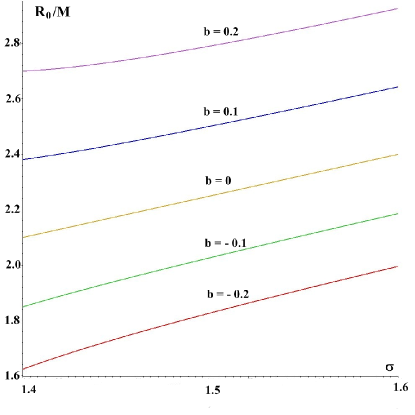
Figure 1: In Case $1$ the wormhole throat is located at $R=R_{0}$. The figure shows that $R_{0}$ increases with $\sigma$. More interesting is that for $b<0$ there is a range of values of $\sigma$ for which $R_{0}<2M$. For $b>0$, $R_{0}>2M$.

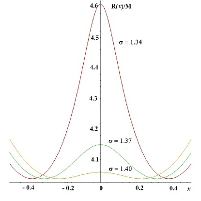
Figure 2: In Case $2$ there are three extremuma, i.e., the spacelike surfaces $R_{(x_{\pm})}$ and $R_{0}$ are turning points for light and all material particles. The figure gives the physical radius as a function of $x$ for $b=0.5$ and the values of $\sigma$ considered in Table $2$. Without loss of generality we have set $m=1$, which is equivalent to introducing a dimensionless coordinate $x\rightarrow x/\sqrt{m}$ in $(30)$. As we approach $r=2m$ we never reach distances $R<R_{(x_{\pm})}=4.038M$ regardless of the choice of $\sigma$, although $R_{(x_{\pm})}$ is attained at different values of $x$. After a re-bounce at $R_{0}$, which does depend on $\sigma$ but corresponds to the same $x$, namely $x=0$, we cross into another space which is the double of the one we started in. The two minimuma coalesce for $\sigma\rightarrow\bar{\sigma}$

Case 2:

When $b\in\left(0,1\right)$ and $2m<r_{0}<\bar{r}$, or what is equivalent $4/3<\sigma<\bar{\sigma}$ , there are three extremuma. One of them is at $x=0$ and corresponds to $R=R_{0}$ given by (33); the other two are at $x=x_{\pm}$ for which

$$R_{(x_{\pm})}=M\sqrt{\frac{b}{a}}\left(\frac{a+b+1}{a+b-1}\right)^{(a+b)/2}>2M.$$ (37)

In this case $\left(1-a-b\right)<0$, therefore from (33) it follows that $R_{0}\rightarrow\infty$ as $\sigma\rightarrow\left(4/3\right)^{+}$. In addition, $R_{0}\rightarrow R_{(x_{\pm})}^{+}$ as $\sigma\rightarrow\bar{\sigma}$, i.e. $R_{0}$ decreases with the increase of $\sigma$, which is in agreement with (35) because in the present case $\sigma<\bar{\sigma}$. What this means is that in this case $R_{(x_{\pm})}$ is a local minimum and $R_{0}$ is a local maximum. This is illustrated in Figure $2$.

As an example, let us choose some particular $b$ in the range $\left(0,1\right)$, e.g. $b=0.5$. For this choice $R_{(x_{\pm})}=4.038M$. Besides, from Table $1$ we get $\bar{\sigma}=1.434$, $(\bar{r}=2.151m)$. In Table $2$ we compute $R_{0}$ for various values of $\sigma$ in the range $1.333<\sigma<1.434$ $(2m<r_{0}<2.151m)$. Similar results, illustrating the fact that $R_{0}>R_{(x_{\pm})}>2M$, can be obtained for other values of $b$ and $\bar{\sigma}$ considered in Table $1$.

Table 2. $R_{0}/M$ for $b=0.5$ and $\sigma\in\left(4/3,1.434\right)$
$\sigma$	$1.34$	$1.37$	$1.40$	$1.43$
$R_{0}/M$	$4.610$	$4.149$	$4.059$	$4.037$

From (36) it follows that, in the present case $(\bar{\sigma}>\sigma)$, the effective EMT satisfies the weak, null and dominant energy conditions in a neighborhood of $x=0$. However, using (32) and Table $1$, it is not difficult to verify that these conditions are now violated in a neighborhood of $x=x_{(\pm)}$, which is where in this case the wormhole throat is located at, as expected.

2.2 Spatial Schwarzschild-Kramer-like solution

In order to generalize the spatial-Schwarzschild metric (7) we now choose

$$B^{2}(r)=\left(1-\frac{2\alpha m}{r}\right)^{-(a+b)},\;\;\;C^{2}(r)=\left(1-\frac{2\alpha m}{r}\right)^{1-a-b},$$ (38)

where $\alpha$ is some positive constant. Substituting these expressions into (4) we obtain a second order differential equation for $A(r)$. To determine the arbitrary constants of integration we impose two conditions. First, that $A\rightarrow 1$ as $r\rightarrow\infty$. Second, that for $a=1$ $(b=0)$ we recover the spatial Schwarzschild solution. With these conditions we obtain

$$A^{2}(r)=\frac{1}{\alpha^{2}}\left[\alpha-1+\left({1-\frac{2\alpha m}{r}}\right)^{(a-b)/2}\right]^{2}\left(1-\frac{2\alpha m}{r}\right)^{b}.$$ (39)

For this solution the total gravitational mass and the PPN parameters are

$$M = m\left[a+b(\alpha-1)\right],$$

$$\beta = \frac{1}{2}\left\{1+\frac{\alpha\left[a^{2}+\alpha b^{2}(\alpha-1)\right]}{\left[a+b\left(\alpha-1\right)\right]^{2}}\right\},$$

$$\gamma = \frac{\alpha(a+b)}{a+b(\alpha-1)}.$$ (40)

The above solution for $\alpha=1$ reduces to the Kramer-like solution (11), and for $\alpha\neq 1$, but $a=1$ $(b=0)$, gives back (7), as expected. In general, for $\alpha\neq 1$, $a\neq 1$ and $b\neq 0$ the quantities $K_{1}$ and $K_{2}$ in (2) behave like $\sim\left[1/(r^{2}Af^{2-a-b})\right]$. Therefore the Kretschmann scalar diverges at $r=0$, $A=0$ and $r=2m\alpha$, as $\left(2-a-b\right)>0$ in the whole range of $b$.

However, there are two cases in which the curvature invariants are regular at $r=2m\alpha$. One of them is $a=1$, $b=0$ discussed by Casadio, Fabbri and Mazzacurati [38], the other case is when $a=0$ and $b=1$. In the latter case the metric (38)-(39) becomes

$$ds^{2}=\frac{1}{\alpha^{2}}\left[1+\left(\alpha-1\right)\sqrt{1-\frac{2\alpha m}{r}}\right]^{2}dt^{2}-\left(1-\frac{2\alpha m}{r}\right)^{-1}dr^{2}-r^{2}d\Omega^{2}.$$ (41)

For $\alpha=1$ we recover the spatial-Schwarzschild wormhole (13) with $R_{0}=2\alpha m$. For $\alpha<1$, the equation $g_{tt}=0$ has no positive solutions for $r$. Thus, there is no horizon. Since the Kretschmann scalar is regular at $r=r_{0}=2\alpha m$, the metric is regularized at $r=r_{0}$ by the substitution $x^{2}=r-r_{0}$. As a result, (41) becomes

$$ds^{2}=\frac{1}{\alpha^{2}}\left[1+\frac{(\alpha-1)|x|}{\sqrt{x^{2}+r_{0}}}\right]^{2}dt^{2}-4\left(x^{2}+r_{0}\right)dx^{2}-(x^{2}+r_{0})^{2}d\Omega^{2},\;\;\;\alpha>1,$$ (42)

which is a symmetric traversable wormhole with throat at $R_{0}=2M\alpha/(\alpha-1)$ and total gravitational mass $M=m\left(\alpha-1\right)$. We emphasize that here $R_{0}>2M$ for all values of $\alpha$.

In order to make contact with other works in the literature, let us notice that the solution for $\alpha=1$ can alternatively be written as

$$ds^{2} = \left[\kappa+\lambda f^{(a-b)/2}\right]^{2}f^{b}dt^{2}-f^{-(a+b)}dr^{2}-r^{2}f^{1-a-b}d\Omega,$$

where $\kappa$ and $\lambda$ are arbitrary constants. The choice $\kappa=0$ and $\lambda=1$ gives back the Kramer-like solution (11); $\lambda=0$ and $\kappa=1$ yields a line element which is similar to (11) with $a$ replaced by $b$ and vice versa. The class of self-dual Lorentzian wormholes discussed in Dadhich et al [19], which in our notation are given by (42), is recovered from (2.2) in the special cases where $a=1$, $b=0$ or $a=0$, $b=1$. This class of solutions is a particular case of the wormhole spacetimes discussed by Bronnikov and Kim [29] in their example $4$.

$\bullet$ A more detailed investigation shows that in the case where $\alpha=1$, there is a family of “spatial Kramer-like solutions” not included in (2.2). Indeed, it is not difficult to verify that the line element

$$ds^{2}=f^{[a+b+\sqrt{1-3ab}]/2}\;dt^{2}-f^{-(a+b)}\;dr^{2}-r^{2}f^{(1-a-b)}\;d\Omega^{2},$$ (44)

also satisfies the field equation (4). Note that $a+b+\sqrt{1-3ab}>0$ for all $a>0$ (i.e., $-2\sqrt{3}\leq b<1$). The Schwarzwschild geometry can be recovered in two distinct limits: either $a=1$, $b=0$ or $a=0$, $b=1$. From an observational point of view this solution is distinct from the ones considered above. This follows from the fact that the PPN parameters are different from the ones calculated in (2.2). Namely, for the line element (44) we find

$$M = \frac{m}{2}\left(a+b+\sqrt{1-3ab}\right),$$

$$\beta = 1,$$

$$\gamma = \frac{2(a+b)}{a+b+\sqrt{1-3ab}}.$$ (45)

$\bullet$ It should be emphasized that we can use any of the above solutions to generate other asymptotically flat solutions to (4) that contain the Schwarzschild spacetime. As an example, let us consider the case where the temporal part of the metric is identical to $g_{tt}$ in the spatial Kramer-like solution (44). From (4) we obtain a first-order differential equation for $B(r)$, which can be easily integrated. The new solution can be written as

$$ds^{2}=f^{[a+b+\sqrt{1-3ab}]/2}\;dt^{2}-\left(\frac{r-\hat{r}}{r-r_{0}}\right)f^{-(a+b)}\;dr^{2}-r^{2}f^{(1-a-b)}\;d\Omega^{2},$$ (46)

with

$$\hat{r}=\frac{m\left[4+3\left(a+b\right)-\sqrt{1-3ab}\right]}{4},\;\;\;\;r_{0}=\frac{3m\sigma}{2}=\mbox{constant},$$

where $\sigma$ is a dimensionless, arbitrary, constant of integration. For $r_{0}=\hat{r}$ the metric (46) reduces to (44). In addition, for $a=1$, $b=0$ the solutions (28) and (46) yield the temporal Schwarzschild metric (6).

It should be noted that $0<\hat{r}<2m$ in the whole range $-2/\sqrt{3}\leq b<1$. The Kretschmann scalar diverges at $r=0$ and $r=2m$, but is regular at $r=\hat{r}$ and $r=r_{0}$. Once again, smooth continuation at $r=r_{0}>2m$, which requires $\sigma>4/3$, is achieved in terms of the coordinate $x$ defined by the relation $r=r_{0}+x^{2}$, viz.,

$$ds^{2}=\left(\frac{x^{2}+r_{0}-2m}{x^{2}+r_{0}}\right)^{[a+b+\sqrt{1-3ab}]/2}\;dt^{2}-\frac{4\left(x^{2}+r_{0}-\hat{r}\right)\left(x^{2}+r_{0}\right)^{a+b}}{\left(x^{2}+r_{0}-2m\right)^{a+b}}\;dx^{2}-\frac{\left(x^{2}+r_{0}\right)^{a+b+1}}{\left(x^{2}+r_{0}-2m\right)^{a+b-1}}\;d\Omega^{2}.$$ (47)

Here the physical radius of a spherical shell with coordinate $x$ is the same as in (30). Therefore, under the same conditions on $b$ and $\sigma$ we have the Cases $1$ and $2$ discussed above. The only difference is that now the total gravitational mass is given by the first equation in (2.2). Therefore, in Case $1$ the wormhole throat is at

$$R_{0}=\frac{3\sigma M}{a+b+\sqrt{1-3ab}}\left(1-\frac{4}{3\sigma}\right)^{(1-a-b)/2},\;\;\;\sigma>4/3.$$ (48)

In case $2$ we now have

$$R_{(x_{\pm})}=\frac{2M\sqrt{ab}}{a+b+\sqrt{1-3ab}}\left(\frac{a+b+1}{a+b-1}\right)^{(a+b)/2}.$$ (49)

One can verify that in Case $2$, the weak, null and dominant energy conditions are satisfied in a neighborhood of $R_{0}$. Once again as in (33) and (37), (i) if $b<0$ we can have $R_{0}<2M$ for a wide range of values of $\sigma$ (see Fig. $1$); (ii) $R_{0}>2M$ for $b>0$ (with $\sigma>\bar{\sigma}$), and (iii) $R_{(x_{\pm})}>2M$ for all $b>0$.

3 Symmetric wormholes from solutions with one regular asymptotic

Let us note that, from a mathematical point of view, the Kramer-like metric (11) and its temporal Schwarzschild generalization (28) differ only by a factor in $g_{rr}$. However, from a physical point of view they are very different: these metrics have distinct PPN parameters and (11) only has one asymptotic region for $b>0$. On the other hand, (28) describes symmetric wormholes in the whole range of $b$ provided $r_{0}>2m$. A similar situation occurs between the spatial Kramer-like solution (44) and its generalization (46). The aim of this section is to generate two more families of traversable symmetric wormholes from solutions that only have one regular asymptotic region.

The new solutions arise from the observation that any solution to the field equation (3) originates new ones given by

$$ds^{2}=A^{2}(r)dt^{2}-h(r)B^{2}(r)dr^{2}-r^{2}C^{2}(r)\;d\Omega^{2},$$ (50)

where

$$h(r)=\left[1+c\;e^{-\int{\frac{B^{2}\;dr}{L^{2}\left(L^{\prime}/L+A^{\prime}/2A\right)}}}\right]^{-1};$$ (51)

$L\equiv rC(r)$, and $c$ is some arbitrary constant.

$\bullet$ First, let us consider the solution (28). If we demand that it must contain the Schwarzschild spacetime for $b=0$ $(a=1)$, then we should set $\sigma=1$. The result is the “temporal Kramer-like” metric

$$ds^{2}=f^{a}\;dt^{2}-\frac{2(f+1)+(f-1)(a+2b)}{1+3f}f^{-(a+b)}\;dr^{2}-r^{2}f^{(1-a-b)}d\Omega^{2}.$$ (52)

We note that $g_{rr}<0$ for any positive $a$. If $a=0$ and $b=1$ $(b=-1)$, the solution describes a wormhole with throat at $R_{0}=3m/2$ $(R_{0}=-m/2,\;m<0)$. In general, for any $b<0$ there is naked singularity at $r=2m$. However, for $b>0$ the physical radius has a minimum at $\bar{r}=m\left(1+a+b\right)>2m$.

Substituting (52) into (51) we generate another solution to (4), namely

$$ds^{2}=f^{a}\;dt^{2}-\left(\frac{r-3m/2}{r-r_{0}}\right)\left[\frac{2(f+1)+(f-1)(a+2b)}{1+3f}\right]f^{-(a+b)}\;dr^{2}-r^{2}f^{(1-a-b)}d\Omega^{2},$$ (53)

where $r_{0}\equiv\left(3m+c\right)/2$.

$\bullet$ Second, we consider the line element (46). If we set $\sigma=1$ we recover the Schwarzschild metric when $b=0$ $(a=1)$. With this choice the solution becomes

$$ds^{2}=f^{[a+b+\sqrt{1-3ab}]/2}\;dt^{2}-\frac{4\left(f+1\right)+\left(f-1\right)\left[3\left(a+b\right)-\sqrt{1-3ab}\right]}{2\left(1+3f\right)}\;f^{-(a+b)}\;dr^{2}-r^{2}f^{(1-a-b)}d\Omega^{2}.$$ (54)

For this metric we find

$$M = \frac{m}{2}\left(a+b+\sqrt{1-3ab}\right),$$

$$\beta = \frac{2+a+b+5\sqrt{1-3ab}}{4(a+b+\sqrt{1-3ab})},$$

$$\gamma = \frac{5(a+b)+2+\sqrt{1-3ab}}{4\left(a+b+\sqrt{1-3ab}\right)}.$$ (55)

Substituting (54) into (51) we get another solution to (4), viz.,

$$ds^{2}=f^{[a+b+\sqrt{1-3ab}]/2}\;dt^{2}-\left(\frac{r-3m/2}{r-r_{0}}\right)\left[\frac{4\left(f+1\right)+\left(f-1\right)\left[3\left(a+b\right)-\sqrt{1-3ab}\right]}{2\left(1+3f\right)}\right]\;f^{-(a+b)}\;dr^{2}-r^{2}f^{(1-a-b)}d\Omega^{2}.$$ (56)

Thus, although the original metrics (52) and (54) only have one regular asymptotic region for $b>0$, the new solutions (53) and (56) in terms of the coordinate $x$ defined by $r=x^{2}+r_{0}$ are regular and symmetric for all values of $b$ and $r_{0}>2m$, so that both $x\rightarrow\infty$ and $x\rightarrow-\infty$ are flat asymptotics. All our symmetric wormholes have a factor proportional to $\left(r-r_{0}\right)^{-1}$ in $g_{rr}$. In this regard, it is interesting to mention a general result obtained by Bronnikov and Kim [29] in curvature coordinates $(g_{\theta\theta}=-R^{2})$. They showed that in traversable, twice asymptotically flat, wormhole solutions the metric function $g_{RR}$ near the throat must behave as $\left(R-R_{0}\right)^{-1}$.

4 Summary

The aim of this work has been to generate new exact static, spherically symmetric Lorentzian wormhole solutions on the brane. Since (4) is a second-order differential equation for $A(r)$ and $C(r)$ and first order for $B(r)$, the simplest way for generating static solutions is to provide some smooth functions $A(r)$ and $C(r)$. Then, the field equation (4) reduces to a linear first-order differential equation for $B(r)$. In the context of curvature coordinates, $C(r)=1$, Bronnikov and Kim [29] have given a thorough discussion of the general conditions on the so-called redshift function $\ln{A(r)}$ under which the solution describes symmetric and asymmetric wormholes.

In this paper, to accomplish our goal we have solved (4) using a different approach: (i) we have relaxed the condition $C(r)=1$, which is required in curvature coordinates. Instead we have chosen $C(r)=f^{(1-a-b)/2}$. From a physical point of view, this choice automatically incorporates the requirement of existence of a throat. Namely, $R(r)=rf^{(1-a-b)/2}$ has at least one regular minimum (a throat) at some $r=\bar{r}>2m$, for $b>0$ (see (20)). In principle, one can always set $C=1$ by redefining the radial coordinate. However, the line element (11) cannot in general (i.e., for any $b\neq 0$) be written in a simple analytical form in terms of the radial coordinate $R=rf^{(1-a-b)/2}$. Therefore, from a practical point of view the choice $C(r)=f^{(1-a-b)/2}$ generates solutions to (4) which are algebraically simple in terms of $r$, but (in general) not expressible in terms of elementary functions of $R$; (ii) we have demanded that the spacetime must contain the Kramer-like spacetime (11), which is a vacuum solution on the brane constructed from the Kaluza-Klein $5D$ solution (8). This assumption guarantees that the Schwarzschild spacetime is recovered for some particular choices of the parameters. We note that in the cosmological realm, $5D$ Kaluza-Klein solutions have been used to generate braneworld cosmological models (with vanishing bulk cosmological constant) via a relatively simple procedure [46].

For $b=0$ and $a=1$ we return to curvature coordinates and our solutions reduce to some well-known ones in the literature. For example, the line element (28) reproduces the temporal Schwarzschild spacetime (6) obtained by Casadio, Fabbri and Mazzacurati [38] in search for new black holes on the brane and by Germani and Maartens [37] as a possible external metric for an isolated braneworld star. Bronnikov and Kim [29], in their example $2$, showed that these spacetimes allow the existence of symmetric traversable wormholes for $r_{0}>2m$ ($R_{0}>2M$ in our notation).

For $b\neq 0$, our solutions display some interesting physical properties:

1. The models with $b<0$ (Case $1$) represent traversable wormholes that can have throats located at $R_{0}<2M$. What this means is that, as seen from outside, a particle or light falling down reaches the Schwarzschild radius (which no longer defines the horizon) in a finite time. It should be noted that in general relativity, in order to have a throat larger (less) than the Schwarzschild radius for a given mass at a flat asymptotic, it is necessary to have matter with negative (positive) energy density [47]. However, for the braneworld wormholes under consideration here this is not necessarily so. Indeed, following the reasoning of [47] we obtain

   $$R_{0}=2\gamma M-8\pi\int_{R_{0}}^{\infty}{R^{2}\rho(R)dR},$$ (57)

   where $\gamma$ is one of the post-Newtonian parameters in the Eddington-Roberston expansion (22). In general relativity $\gamma=1$, but in our braneworld solutions it can be less or bigger than $1$ depending on the choice of various parameters (see, e.g. (2.1)).

2. The models with $b>0$ (Case $2$) are wormhole spacetimes which have three extremal spheres with finite area. This is in contrast to standard Lorenzian wormholes, a la Morris and Thorne, that have only one extremal surface of minimal area which is identified with the throat. Here, although the wormholes are symmetrical and twice asymptotically flat the throat is not located at $x=0$, as in [29] and [38], but instead is located at some $x\neq 0$ which explicitly depends on the choice of $\sigma$. However, the specific value of the wormhole radius is the same for the whole range $4/3<\sigma<\bar{\sigma}$; it depends only on the choice of $b>0$ (see equations (37), (49)). We note that the extremal spheres have radii larger than $2M$ in the whole range of allowed parameters $b$ and $\sigma$. These conclusions concerning the Case $2$ are neatly summarized by figure $2$.

The two-parameter solutions (28), (46), (53), (56) share similar properties, viz., for different values of $b$ (or $a$) and $\sigma$ they can describe black holes, naked singularities and symmetric traversable wormholes of the types discussed in Cases $1$ and $2$. However, from an experimental point of view they are not equivalent. This follows from the fact that the PPN parameters and the total masses are distinct in each of these solutions. Analogous characteristics show the one-parameter solutions (11), (44), (52), (54) which yield the Schwarzschild spacetime for $b=0$, naked singularities for $b<0$ and configurations that only have one asymptotically flat region for $b>0$.

From a formal point of view the symmetric solutions are obtained from those with only one asymptotic region by replacing in the latter $g_{rr}\rightarrow\left(\frac{r-r_{s}}{r-r_{0}}\right)g_{rr}$ and keeping the other metric functions fixed. Here $r_{0}>2m$ is an arbitrary parameter, and $r_{s}$ is a constant determined by the field equations, which in all cases turns to be less than $2m$. Besides the geometric differences discussed above, the effective matter is quite different in both cases. In particular, configurations with only one asymptotic region have $T_{0}^{0}<0$ everywhere (but their total gravitational mass $M$ is positive), while the symmetric wormholes have positive effective energy density.

Thus, in this work we have obtained a number of models for wormholes on the brane with interesting physical properties. One can use them to generate new ones by means of iteration. We note that, although we have restricted our study to the solutions engendered by the Kramer-like metric (11) for which $C=A^{(1-a-b)/a}$, our discussion can be generalized by considering $C\propto A^{p}$, where $p$ is some constant parameter (not necessarily $p=(1-a-b)/a$). With this assumption we can follow the general approach of Bronnikov and Kim [29] to study how to choose $A(r)$ in (4) to obtain solutions satisfying wormhole conditions.

The next logical step, to obtain a complete wormhole model within the braneworld paradigm, is to investigate the extension of our solutions into the bulk. However, finding an exact solution in $5D$ which is consistent with a particular metric in $4D$ is not an easy task. In spite of this, the existence of such a solution is guaranteed by the Campbell-Magaard’s embedding theorems [48]. The coupling of our wormholes solutions to the bulk geometry, though important, is beyond the scope of the present paper.

Acknowledgments:

I wish to thank Kirill Bronnikov for helpful comments and constructive suggestions.

References

- [1] http://en.wikipedia.org/wiki/Wormholes_in_fiction
- [2] http://en.wikipedia.org/wiki/Time_travel_in_science_fiction
- [3] J.A. Wheeler, “Geons”, Phys. Rev. 97 (1955) 511.
- [4] J.A. Wheeler, Geometrodynamics, Academic Press, New York (1962).
- [5] M.S. Morris, K.S. Thorne and U. Yurtsewer, “Wormholes, time machines, and the weak energy condition”, Phys. Rev. Lett. 61 (1988) 1446.
- [6] M.S. Morris and K.S. Thorne, “Wormholes in spacetime and their use for interstellar travel: A tool for teaching general relativity”, Am. J. Phys. 56 (1988) 395.
- [7] S.A. Hayward, “Dynamic wormholes”, Int. J. Mod. Phys. D 8 (1999) 373 [arXiv:gr-qc/9805019]
- [8] N.S. Kardashev, I.D. Novikov and A.A. Shatskiy, “Astrophysics of wormholes”, Int. J. Mod. Phys. D 16 (2007) 909 [arXiv:astro-ph/0610441].
- [9] P.K.F. Kuhfittig, “Could some black holes have evolved from wormholes?”, Schol. Res. Exch. (2008) 296158 [arXiv:0812.4712].
- [10] S.V. Sushkov and O.B. Zaslavskii, “Horizon closeness bounds for static black hole mimickers”, Phys. Rev. D 79 (2009) 067502 [arXiv:0903.1510].
- [11] D. Hochberg and M. Visser, “The null energy condition in dynamic wormholes”, Phys. Rev. Lett. 81 (1998) 746 [arXiv:gr-qc/9802048].
- [12] D. Hochberg and M. Visser, “General dynamic wormholes and violation of the null energy condition”, [arXiv:gr-qc/9901020].
- [13] D. Hochberg and M. Visser, “Dynamic wormholes, anti-trapped surfaces, and energy conditions”, Phys. Rev. D 58 (1998) 044021 [arXiv:gr-qc/9802046].
- [14] C. Barcelo and Matt Visser, “Traversable wormholes from massless conformally coupled scalar fields”, Phys. Lett. B466 (1999) 127 [arXiv:gr-qc/9908029].
- [15] S.V. Sushkov and S.-W. Kim, “Wormholes supported by the kink-like configuration of a scalar field”, Class. Quant. Grav. 19 (2002) 4909 [arXiv:gr-qc/0208069].
- [16] P.K.F. Kuhfittig, “A single model of traversable wormholes supported by generalized phantom energy or Chaplygin gas ”, Gen.Rel.Grav. 41 (2009) 1485 [arXiv:0904.3566].
- [17] K.A. Bronnikov, “Scalar-tensor theory and scalar charge”, Acta. Phys. Pol. B 4 (1973) 251.
- [18] H. Ellis, “Ether flow through a drainhole - a particle model in general relativity”, J. Math. Phys. 14 (1973) 104.
- [19] N. Dadhich, S. Kar, S. Mukherji and M. Visser, “R=0 spacetimes and self-dual Lorentzian wormholes”, Phys. Rev. D 65 (2002) 064004 [arXiv:gr-qc/0109069].
- [20] K. K. Nandi, B. Bhattacharjee, S. M. K. Alam and J. Evans, “Brans-Dicke wormholes in the Jordan and Einstein frames”, Phys. Rev. D 57 (1998) 823.
- [21] L.A. Anchordoqui, A.G. Grunfeld and D.F. Torres, “Vacuum static Brans-Dicke wormhole” Grav.Cosmol. 4 (1998) 287 [arXiv:gr-qc/9707025].
- [22] D. Hochberg, “Lorentzian wormholes in higher order gravity theories” Phys. Lett. 251 (1990) 349.
- [23] D. Hochberg, A. Popov and S. V. Sushkov, “Self-consistent wormhole solutions of semiclassical gravity”, Phys. Rev. Lett. 78 (1997) 2050 [arXiv:gr-qc/9701064].
- [24] R. Garattini and F. S. N. Lobo, “Self sustained phantom wormholes in semi-classical gravity”, Class. Quant. Grav. 24 (2007) 2401 [arXiv:gr-qc/0701020].
- [25] K.A. Bronnikov and A.A. Starobinsky, “No realistic wormholes from ghost-free scalar-tensor phantom dark energy”, JETP Lett. 85 (2007) 1 [arXiv:gr-qc/0612032].
- [26] V. Dzhunushaliev and D. Singleton, “Wormholes and flux tubes in 5D Kaluza-Klein theory”, Phys. Rev. D 59 (1999) 064018 [arXiv:gr-qc/9807086].
- [27] B. Bhawal and S. Kar, “Lorentzian wormholes in Einstein-Gauss-Bonnet theory”, Phys. Rev. D 46 (1992) 2464.
- [28] G. Dotti, J. Oliva and R. Troncoso, “ Static wormhole solution for higher-dimensional gravity in vacuum”, Phys. Rev. D 75 (2007) 024002 [arXiv:hep-th/0607062].
- [29] K.A. Bronnikov and Sung-Won Kim, “Possible wormholes in a braneworld”, Phys. Rev. D 67 (2003) 064027 [arXiv:gr-qc/0212112].
- [30] F. S. N. Lobo, “A general class of braneworld wormholes”, Phys. Rev. D 75 (2007) 064027 [arXiv:gr-qc/0701133].
- [31] L. Randall and R. Sundrum, “An alternative to compactification”, Phys. Rev. Lett. 83 (1999) 4690 [arXiv:hep-th/9906064].
- [32] T. Shiromizu, K. Maeda and M. Sasaki, “The Einstein equations on the 3-Braneworld”, Phys. Rev. D 62 (2000) 024012 [arXiv:gr-qc/9910076].
- [33] L.D. Landau and E.M. Lifshitz, The Classical Theory of Fields, 4th edn. (Butterworth-Heinemann, 2002).
- [34] D. N. Vollick, “Negative Energies on the Brane”, Gen. Rel. Grav. 34 (2002) 1 [arXiv:hep-th/0004064].
- [35] K.A. Bronnikov, H. Dehnen and V.N. Melnikov, “On a general class of braneworld black holes”, Phys. Rev. D 68 (2003) 024025 [arXiv:gr-qc/0304068].
- [36] M. Visser and D.L. Wiltshire, “On-brane data for braneworld stars”, Phys. Rev. D 67 (2003) 104004 [arXiv:hep-th/0212333].
- [37] C. Germani and R. Maartens, “Stars in the braneworld”, Phys. Rev. D 64 (2001) 124010 [arXiv:hep-th/0107011].
- [38] R. Casadio, A. Fabbri, L. Mazzacurati, “New black holes in the brane-world?”, Phys. Rev. D 65 (2002) 084040 [arXiv:gr-qc/0111072].
- [39] J. Ponce de Leon, “Stellar models with Schwarzschild and non-Schwarzschild vacuum exteriors”, Grav. Cosmol. 14 (2008) 65 [arXiv:0711.0998].
- [40] J. Ponce de Leon, “Static exteriors for nonstatic braneworld stars”, Class. Quant. Grav. 25 (2008) 075012 [arXiv:0711.4415].
- [41] K.A. Bronnikov and J.P.S. Lemos, “Cylindrical wormholes”, Phys. Rev. D 79 (2009) 104019 [arXiv:0902.2360].
- [42] J. Ponce de Leon, “Kaluza-Klein solitons reexamined”, Int. J. Mod. Phys. D 17 (2008) 237 [arXiv:gr-qc/0611082].
- [43] D. Kramer, “Axialsymmetric stationary solutions of the Projective Field Theory”, Acta Phys. Pol. B 2 (1970) 807 (In German).
- [44] S. Weinberg, Gravitation and Cosmology, John Wiley & Sons, 1972, page 183.
- [45] C.M. Will, “The confrontation between general relativity and experiment”, Living Rev. Rel. 4 (2001) 4 [arXiv:gr-qc/0103036].
- [46] J. Ponce de Leon, “Equivalence Between Space-Time-Matter and Brane-World Theories”, Mod.Phys.Lett. A 16 (2001) 2291 [arXiv:gr-qc/0111011].
- [47] K.A. Bronnikov and S.G. Rubin, Lectures on Gravitation and Cosmology, MIFI Press, Moscow, 2008 (in Russian), pages 171-172.
- [48] S. Rippl, C. Romero, R. Tavakol, “D-dimensional gravity from (D + 1) dimensions”, Class.Quant.Grav. 12 (1995)2411, arXiv:gr-qc/9511016; J.E. Lidsey, C. Romero, R. Tavakol, S. Rippl, “On applications of Campbell’s embedding theorem”, Class.Quant.Grav. 14 (1997)865, arXiv:gr-qc/9907040; S.S. Seahra, P.S. Wesson, “Application of the Campbell-Magaard theorem to higher-dimensional physics”, Class. Quant. Grav. 20 (2003)1321, arXiv:gr-qc/0302015 ; F. Dahia, C. Romero, “Dynamically generated embeddings of spacetime”, Class.Quant.Grav. 22 (2005)5005, arXiv:gr-qc/0503103.