Transport properties of partially equilibrated quantum wires

Abstract

We study the effect of thermal equilibration on the transport properties of a weakly interacting one-dimensional electron system. Although equilibration is severely suppressed due to phase-space restrictions and conservation laws, it can lead to intriguing signatures in partially equilibrated quantum wires. We consider an ideal homogeneous quantum wire. We find a finite temperature correction to the quantized conductance, which for a short wire scales with its length, but saturates to a length-independent value once the wire becomes exponentially long. We also discuss thermoelectric properties of long quantum wires. We show that the uniform quantum wire is a perfect thermoelectric refrigerator, approaching Carnot efficiency with increasing wire length.

I Introduction

The quantization of the dc conductance in ballistic quantum wires, first observed about two decades ago,cq1 ; cq2 is one of the fundamental discoveries of mesoscopic physics. The staircase-like dependence of the conductance on the electron density, with plateaus at integral numbers of $2e^{2}/h$ is readily understood from the single-electron picture.landauer The latter associates each plateau with a fixed number of occupied electronic subbands, each supplying one quantum of conductance $2e^{2}/h$. On the other hand, interactions between one-dimensional electrons often lead to qualitatively new phenomena. These are commonly described within the so-called Luttinger liquid theory,giamarchi drastically different from Landau’s Fermi liquid description applicable to higher-dimensional systems. The remarkable success of the simple single-electron picture in describing the quantization of conductance is attributed to the fact that quantum wires are always connected to two-dimensional leads, where interactions between electrons do not play a significant role. In fact, it was shown in Refs. [maslov, ; safi, ; ponomarenko, ] that in an ideal Luttinger liquid connected to Fermi liquid leads, the dc conductance is completely controlled by the latter and, therefore, is not affected by interactions in the wire.

For that reason, the discovery of small temperature-dependent deviations from perfect quantization0.7-1 ; 0.7-2 ; 0.7-3 ; 0.7-4 ; 0.7-5 ; 0.7-6 ; 0.7-7 ; 0.7-8 ; 0.7-9 of the conductance of quantum wires at low electron densities raised a lot of interest. These generally manifest themselves as a shoulder-like structure just below the first plateau of conductance. Weak at the lowest temperatures available, this feature becomes more significant as the temperature is increased, turning into a quasi-plateau at about $0.7\times(2e^{2}/h)$. A number of theoretical efforts trying to reveal the microscopic mechanism of this so-called “0.7 structure” have been made. Several spin-related approaches attribute the effect to spontaneous polarization of the electron spins in the wire0.7-1 ; spinpol1 ; spinpol2 or the existence of a local spin-degenerate quasi-bound state playing the role of a Kondo impurity.kondo1 ; kondo2 Other approaches discuss the role of scattering from plasmons,plasmons spin waves,spinwaves or phonons.phonons

Despite the absence of a commonly accepted microscopic theory, it is generally recognized that electron-electron interactions must be included to account for the effect. As a consequence, a number of recent publications reconsider the effect of interactions on the transport properties of one-dimensional conductors, going beyond the picture of an ideal Luttinger liquid.jerome1 ; jerome2 ; jerome3 ; lunde1 ; lunde2 ; wang ; spivak ; bruus ; tokura ; meir ; meidan ; syljuasen ; matveev1 ; mirlin Here we focus on a very fundamental aspect of interactions, studying how they lead to the equilibration inside the wire of electrons coming from the two leads. We emphasize that this effect is absent in an ideal Luttinger liquid. Indeed, the bosonic elementary excitations of the Luttinger liquid have infinite lifetime, thus there is no relaxation towards equilibrium in these systems, no matter how strong the interactions. Within the Luttinger-liquid theory the processes leading to the equilibration of the electron system would be accounted for by the additional terms in the Hamiltonian, which are irrelevant in the renormalization group sense. Instead of pursuing this strategy, we consider the regime of weakly interacting electrons, thereby avoiding the complexity of the Luttinger-liquid picture.

Non-interacting electrons propagate ballistically through the wire and, therefore, keep memory of the lead they originated from. Thus the distribution function of electrons inside the wire depends on the direction of motion. For the right- and left-moving particles it is controlled, respectively, by the left and right lead:

$$f_{p}^{(0)}=\frac{\theta(p)}{e^{(\epsilon_{p}-\mu_{l})/T}+1}+\frac{\theta(-p)}{e^{(\epsilon_{p}-\mu_{r})/T}+1}.$$ (1)

Here $\epsilon_{p}$ is the energy of an electron with momentum $p$ and $\theta(p)$ is the unit step function. The left and right leads are assumed to have the same temperature $T$, but different chemical potentials $\mu_{l}=\mu+eV$ and $\mu_{r}=\mu$ (see Fig. 1). Using the distribution function (1) one easily finds the electric current $I=G_{0}V$, with the conductance

$$G_{0}=\frac{2e^{2}}{h}\frac{1}{e^{-\mu/T}+1},$$ (2)

which coincides with the well-known conductance quantum $2e^{2}/h$ up to an exponentially small correction $\sim e^{-\mu/T}$.

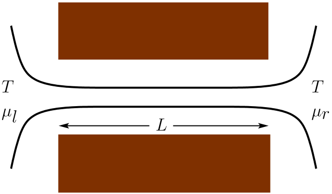
Figure 1: Schematic picture of the quantum wire of length $L$ which is formed by confining a two-dimensional electron gas with gates (dark regions). Electrons in the left and right lead are described by Fermi distribution functions characterized by temperature $T$ and chemical potentials $\mu_{l}$ and $\mu_{r}$, respectively.

In the presence of interactions, the ballistic propagation of electrons through the wire may be interrupted by collisions with other electrons. As a result of these collisions, some electrons change their direction of motion thus losing the memory of the lead they originated from. Such scattering processes modify the electron distribution function which is then no longer given by Eq. (1). The effect of the electron-electron collisions on the distribution function depends strongly on the length of the wire. Indeed, electrons traverse short wires relatively fast, so the interactions do not have the time to change distribution (1) considerably. On the other hand, in the limit of a very long wire one should expect full equilibration of left- and right-moving electrons into a single distribution, even in the case of weak interactions.

To simplify the subsequent discussion, in this paper we consider the case of electrons with quadratic spectrum, $\epsilon_{p}=p^{2}/2m$, where $m$ is the electron effective mass. Then the system is Galilean invariant, and one can easily infer the electron distribution function in the fully equilibrated state. Viewed from a frame moving with the drift velocity $v_{d}=I/ne$ (where $I$ is the electric current and $n$ is the electron density) the electron system is at rest and must be described by the equilibrium Fermi distribution. Performing a Galilean transformation back into the stationary frame of reference this distribution takes the form

$$f_{p}=\frac{1}{e^{(\epsilon_{p}-v_{d}p-\bar{\mu})/{\cal T}}+1},$$ (3)

where the chemical potential $\bar{\mu}$ and temperature ${\cal T}$ inside the equilibrated wire are, in general, different from $\mu_{l/r}$ and $T$. At zero temperature, $T={\cal T}=0$, the distributions (1) and (3) coincide, provided $\mu_{l/r}=\bar{\mu}\pm v_{d}p_{F}$, where $p_{F}=\pi\hbar n/2$ is the Fermi momentum of the system. At non-zero temperature the distribution function (3) of electrons inside the wire is slightly different from the distribution (1) supplied by the leads. In a previous workjerome3 we have shown that the mismatch of the distribution functions inside a very long wire and in the leads results in additional contact resistance, reducing the conductance to

$$G_{\infty}=\frac{2e^{2}}{h}\left[1-\frac{\pi^{2}}{12}\left(\frac{T}{\mu}\right)^{2}\right].$$ (4)

It is worth noting that the quadratic in $T/\mu$ correction in Eq. (4) is much more significant than the exponentially small correction in Eq. (2).

The mechanism of equilibration of the electron distribution function in one dimension is not fully understood. While in higher dimensional systems equilibration at low temperature is primarily provided by pair collisions of electrons, these do not provide a relaxation mechanism in one dimension. This is due to the conservation laws for momentum and energy which severely restrict the phase-space available for scattering processes, Fig. 2(a). As a result, pair collisions in one-dimensional wires can only occur with a zero momentum exchange or an interchange of the two momenta, leaving the distribution function unaffected. The leading equilibration mechanism thus involves collisions of more than two particles. For a weakly interacting system, it is then natural to assume that equilibration is provided by three-electron scattering processes.

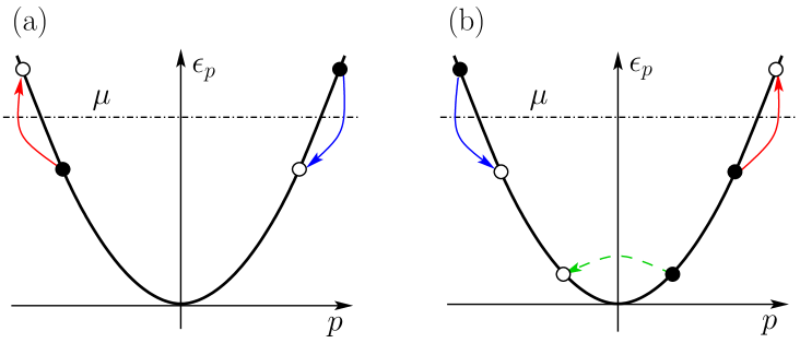
Figure 2: (a) Energy-conserving two-particle scattering process violates conservation of momentum. Such processes can occur only in inhomogeneous systems. (b) Dominant three-particle collision which gives rise to corrections to the conductance of short quantum wires.lunde1 A hole at the bottom of the band scatters off electron excitations close to the Fermi level.

The effect of three-particle collisions on the transport properties of short wires has been studied in a recent work by Lunde, Flensberg, and Glazman.lunde1 In such short systems the effect of equilibration is weak and the distribution function can be calculated perturbatively from the distribution of non-interacting electrons (1) within the Boltzmann equation framework. Following this approach, Lunde et al.lunde1 obtained interaction-induced corrections to transport, which they attributed to specific three-particle scattering events that change the number of left- and right-movers. Indeed, in the absence of interactions, the current flowing through the system can be viewed as the superposition of the right- and left-moving flows of electrons supplied by the left and right leads, respectively. Once interactions are included, these individual contributions change due to electron-electron collisions, and one needs to account for the fact that electrons can now change direction. The electric current flowing through the wire is thus given by the sum of the non-interacting part $I_{0}=G_{0}V$, and the change in, say, the number of right-moving electrons inside the wire

$$I=G_{0}V+e\dot{N}^{R}.$$ (5)

Interaction-induced corrections to transport therefore arise from processes which change the number of right- and left-moving electrons rather than a change in the velocity of the charge carriers, as also pointed out in Ref. [lunde1, ].

As shown by Lunde et al.,lunde1 the most efficient three-particle process changing the number of right-moving electrons involves scattering of an electron into an empty state near the bottom of the band, see Fig. 2(b). By calculating the resulting $\dot{N}^{R}$, they obtained the correction to the conductance (2) of the wire of the form

$$\delta G=-\frac{2e^{2}}{h}\,\frac{L}{l_{eee}}\,e^{-\mu/T},$$ (6)

where the length $l_{eee}$ is determined by the interaction strength and shows a power-law temperature dependence. The exponential smallness of the correction (6) is due to the small probability of finding an empty state near the bottom of the band. Since the small backscattering probability grows linearly with the length $L$, the correction $\delta G\propto L$.

Because the same three-particle processes are responsible for the thermal equilibration of the distribution (1) into (3), the papers Ref. [jerome3, ] and Ref. [lunde1, ] reviewed above study the same physical phenomenon, albeit in the opposite limits of a long and a short wire. In the present paper we bridge the gap between these two limits. We discuss how the electron distribution evolves from the out-of-equilibrium form (1) in a short wire to a fully equilibrated form (3) in a long wire, and study how transport is affected by the process of equilibration. Our analysis focuses on weak electron-electron interactions. It is thus formulated entirely in terms of electrons, and does not use the bosonization technique.

The paper is organized as follows. In sections II and III we investigate how the conductance changes with increasing length of the wire. In Sec. II we expand on the kinetic-equation treatmentlunde1 of backscattering in short wires and study the length dependence of the conductance while the correction $\delta G$ remains exponentially small. In section III we turn to the regime of exponentially long wires, where the correction $\delta G\sim(e^{2}/h)(T/\mu)^{2}$, cf. Eq. (4). In section IV we study the thermoelectric effects and show that the uniform quantum wire is a perfect thermoelectric refrigerator, attaining Carnot efficiency with increasing wire length. Details of some calculations can be found in the Appendices.

II Conductance of short wires

Consider a quantum wire of length $L$, connected by ideal reflectionless contacts to non-interacting leads biased by voltage $V$. We are interested in the process of thermal equilibration of the electrons inside the wire, i.e., in how the transition from distribution (1) to (3) occurs, and how it affects the transport properties of the system.

Following Lunde et al.,lunde1 we describe the electron transport in the wire in the framework of the Boltzmann equation

$$\frac{p}{m}\frac{\partial f_{p,x}}{\partial x}=I_{p,x}[f].$$ (7)

We consider the steady-state setup in which the electron distribution function $f_{p,x}$ depends on the position $x$ along the wire, but not on time. The collision integral $I_{p,x}[f]$ is, in general, a nonlinear functional of the distribution function, whose form is determined by the scattering processes affecting the distribution function. As discussed above, in our case the dominant processes are three-particle collisions, in which case

$$I_{p_{1},x}[f]=-\sum_{\footnotesize\begin{array}[]{l}p_{2},p_{3},\\ \sigma_{2},\sigma_{3}\end{array}}\sum_{\footnotesize\begin{array}[]{l}p^{\prime}_{1},p^{\prime}_{2},p^{\prime}_{3}\\ \sigma^{\prime}_{1},\sigma^{\prime}_{2},\sigma^{\prime}_{3}\end{array}}w_{123;1^{\prime}2^{\prime}3^{\prime}}\left[f_{1}f_{2}f_{3}\left(1-f_{1^{\prime}}\right)\left(1-f_{2^{\prime}}\right)\left(1-f_{3^{\prime}}\right)-f_{1^{\prime}}f_{2^{\prime}}f_{3^{\prime}}\left(1-f_{1}\right)\left(1-f_{2}\right)\left(1-f_{3}\right)\right],$$ (8)

where $w_{123;1^{\prime}2^{\prime}3^{\prime}}$ is the rate for scattering the set of incoming states $\{p_{1}\sigma_{1},p_{2}\sigma_{2},p_{3}\sigma_{3}\}$ into the set of outgoing states $\{p^{\prime}_{1}\sigma^{\prime}_{1},p^{\prime}_{2}\sigma^{\prime}_{2},p^{\prime}_{3}\sigma^{\prime}_{3}\}$, and for notational convenience we shortened $f_{i}=f_{p_{i},x}$.

The Boltzmann equation (7) should be solved with the boundary conditions stating that the distributions $f_{p,0}$ of the right-moving electrons ($p>0$) at the left end of the wire and $f_{p,L}$ of the left-moving electrons ($p<0$) at the right end coincide with the distribution function $f_{p}^{(0)}$ in the leads, Eq. (1). The conductance of the wire can then be found from Eq. (5), with the rate of change in the number of right-moving electrons related to the collision integral via

$$\dot{N}^{R}=2\int_{0}^{L}dx\int_{0}^{\infty}{dp\over h}I_{p,x}[f].$$ (9)

Solving the Boltzmann equation exactly is a very difficult problem due to the non-linearity of the collision integral (8), so one generally has to make some simplifying assumptions. Such assumption in our case is that the temperature $T$ is small compared to the chemical potential $\mu$.

Clearly, at $T=0$ no real scattering processes are allowed, and the unperturbed distribution $f_{p}=\theta(p_{F}-|p-mu|)$ solves the Boltzmann equation (7) for any value of the drift velocity $u$. Since in this case the collision integral $I_{p,x}[f]$ vanishes, we get $\dot{N}^{R}=0$, and, according to (5), the conductance of the wire is $2e^{2}/h$.

A finite temperature $T$ acts in two important ways. First, it affects states near the Fermi level: the step in the zero-$T$ distribution softens, providing partially occupied states in a momentum range $\delta p\sim T/v_{F}$ around the Fermi points. Secondly, it ensures a finite occupation of a hole (i.e., a vacant state) near the bottom of the band. Although the occupation probability of such a hole is exponentially small, $1-f_{p}\sim e^{-\mu/T}$, its presence is crucial for the three-particle processes that change the number of right-moving electrons, see Fig. 2(b). It is important to realize that the backscattering of holes is accompanied by scattering of electrons near the Fermi points, Fig. 2(b). In fact, this is the mechanism of the equilibration of the distribution function to the form (3) in long wires. Although the backscattering rate is exponentially small, $\dot{N}^{R}\propto e^{-\mu/T}$, it scales with the length of the wire. Thus the full equilibration is achieved in wires whose length $L$ exceeds an exponentially long equilibration length $l_{\rm eq}\propto e^{\mu/T}$. The exact definition of $l_{\rm eq}$ will be given below, see Eq. (59).

In this section we will discuss the case of short wires, $L\ll l_{eq}$. The regime $L\gtrsim l_{\rm eq}$ will be discussed in Sec. III.

II.1 Very short wires

We start our discussion with the case of very short wires, recently considered by Lunde, Flensberg, and Glazman.lunde1 The authors argued that for short enough wires, the interactions have little time to change the distribution function from its initial value $f_{p}^{(0)}$ given by Eq. (1), allowing one to perform a perturbative expansion in the scattering rate $w_{123;1^{\prime}2^{\prime}3^{\prime}}$. In the lowest order, this amounts to approximating the collision integral as

$$I_{p,x}[f]\simeq I_{p,x}[f^{(0)}].$$ (10)

Solving the Boltzmann equation to this approximation, they obtained an expression for the modified distribution function inside the wire, which they used to compute the electric current to first order in the scattering rate.

The resulting correction to the conductance of the wire has the form (6), in which microscopic details of the interaction potential are absorbed into the length $l_{eee}$. Lunde et al.lunde1 performed their calculation for a specific model of electrons interacting via a potential defined by its Fourier transform $V_{q}=V_{0}(1-q^{2}/q_{0}^{2})$. This expression results from the expansion of a general potential under the assumption that small-momentum scattering is dominant. The parameter $q_{0}\ll k_{F}$ accounts for the screening by the nearby metallic gates, while $V_{0}$ is the zero-momentum Fourier component of the screened Coulomb potential. Within this model, the length $l_{eee}$ is given bylunde1

$$l_{eee}^{-1}\sim{\left(V_{0}k_{F}\over\mu\right)^{4}}\left({k_{F}\over q_{0}}\right)^{4}\left({T\over\mu}\right)^{7}k_{F}.$$ (11)

A more careful treatment of the Coulomb interaction screened by a gate leads to an additional logarithmic temperature dependence in Eq. (11), see Appendix A.

To better understand the result (6) and find the limits of its applicability, we discuss the qualitative picture of this phenomenon. Let us focus on a single three-electron collision process. The most favorable collision involves a maximal number of states close to the Fermi points. However, due to the conservation of both energy and momentum, collisions that change the number of right- and left-movers cannot occur near the Fermi level, and have to involve states deep in the electron band. As pointed out by Lunde et al.,lunde1 the scattering process most susceptible to alter the current thus typically scatters two electrons close to the Fermi points and one electron at the bottom of the band, as schematically depicted in Fig. 2(b). It is convenient to think of this collision as a process in which a deep hole, corresponding to the outgoing electron state, is backscattered by electron excitations close to the Fermi level. These excitations are typically associated with a momentum change $|\delta p|\sim T/v_{F}$ due to Fermi-blocking, so that the backscattering occurs over a distance $\sim T/v_{F}$ in momentum space. Let us furthermore characterize this process by introducing a scattering rate $1/\tau_{0}$, which can be approximated by a constant since the initial and final states both lie at the bottom of the band.

The change $\dot{N}^{R}$ in the number of right-moving electrons per unit time, due to these three-particle collisions can then be readily obtained. It is given by the product of the scattering rate $1/\tau_{0}$ for one such collision times the number of deep holes susceptible to be backscattered. The latter can be estimated from the probability to find a left- or right-moving hole $e^{-\mu^{L,R}/T}$ and the number of states ${(T/v_{F})/(h/{L})}$ available within the typical momentum range of the backscattering process. Taking into account that the scattering of a left- or a right-moving hole both contribute to $\dot{N}^{R}$, but with a different sign, one finally has

$$\dot{N}^{R} = \frac{2}{\tau_{0}}\left(e^{-\mu^{R}/T}-e^{-\mu^{L}/T}\right)\frac{TL}{hv_{F}}$$ (12)

$$= -{2\over\tau_{0}}{\Delta\mu\over hv_{F}}e^{-\mu/T}L,$$

where $\Delta\mu=\mu^{R}-\mu^{L}$, and we absorbed potential numerical prefactors into the definition of $\tau_{0}$. Throughout this paper we use subscripts $l$ and $r$ to denote the left and right leads, whereas superscripts $L$ and $R$ refer to the left- and right-moving electrons. In short wires the chemical potentials of electrons are not significantly affected by the scattering processes, so $\mu^{R}=\mu_{l}$, $\mu^{L}=\mu_{r}$, and $\Delta\mu=eV$.

We then notice that according to Eq. (5) the correction to the conductance of the wire due to the backscattering processes is $\delta G=e\dot{N}^{R}/V$. As a result we recover the result (6) of Lunde et al.,lunde1 provided

$$\tau_{0}\sim\frac{l_{eee}}{v_{F}}.$$ (13)

The derivation of Eq. (6) relied on the assumption that the occupation probability of a deep hole is well described by the distribution of non-interacting particles, or, alternatively, that one can approximate the collision integral according to Eq. (10). This approximation holds in cases where the hole typically scatters no more than once during its propagation through the wire, and any transition between subsystems of left- and right-movers occurs in a single collision. One thus expects this result to be valid for wires shorter than the mean free path of the hole $l_{0}$. Since the typical momentum of a hole contributing to $\dot{N}^{R}$ is of order $T/v_{F}$, we estimate $l_{0}\sim T\tau_{0}/p_{F}$. Substituting the estimate (13), we obtain

$$l_{0}\sim\frac{T}{\mu}\,l_{eee}.$$ (14)

For the particular model of the interaction potential used in Ref. [lunde1, ] we estimate

$$l_{0}^{-1}\sim{\left(V_{0}k_{F}\over\mu\right)^{4}}\left({k_{F}\over q_{0}}\right)^{4}\left({T\over\mu}\right)^{6}k_{F}.$$ (15)

In wires longer than $l_{0}$, holes near the bottom of the band experience multiple collisions while they propagate through the wire, the distribution function deviate significantly from the unperturbed form (1), and the result (6) is no longer applicable.

II.2 Longer wires: $l_{0}\ll L\ll l_{\rm eq}$

In wires longer than $l_{0}$ a typical hole near the bottom of the band is scattered many times while traversing the wire. Each collision changes its momentum by a small amount $\delta p\sim T/v_{F}\ll p_{F}$, with a sign that varies in a random fashion. The hole thus performs a random walk in momentum space. This picture is analogous to the diffusion of a Brownian particle in air. In the latter case, the change of momentum of the particle in each collision is small because its mass is much larger than that of the air molecules. Similarly to the case of Brownian motion, one can use the small parameter $\delta p/p_{F}\sim T/\mu$ to bring the collision integral of holes to a much simpler Fokker-Planck form

$$I_{p,x}[g]\simeq-\frac{\partial}{\partial p}\left(A(p)g_{p,x}-{1\over 2}\frac{\partial}{\partial p}[B(p)g_{p,x}]\right),$$ (16)

where we introduced the hole distribution $g_{p,x}=1-f_{p,x}$. The functions $A(p)$ and $B(p)$ entering Eq. (16) are model specific. In the case of three-electron collisions they can be determined explicitly. They depend on the three-particle scattering rate as well as the electron distribution function in the vicinity of the Fermi level. The latter can be assumed to be unperturbed by the collisions in the wire as long as $L\ll l_{\rm eq}\propto e^{\mu/T}$. The resulting derivation of $A(p)$ and $B(p)$ can be found in Appendix B; here we provide order of magnitude estimates.

First we notice that $B(p)$ has the physical meaning of the diffusion coefficient in momentum space, i.e., the typical momentum change of a hole over time $t$ behaves as $(\Delta p)^{2}\sim Bt$. Assuming as before that the hole changes its momentum by $\pm T/v_{F}$ once during time $\tau_{0}$, we conclude that $(\Delta p)^{2}\sim(T/v_{F})^{2}t/\tau_{0}$ for $t\gg\tau_{0}$. Thus we estimate

$$B\sim\frac{T^{2}}{v_{F}^{2}\tau_{0}}\sim\frac{T^{2}}{v_{F}l_{eee}},$$ (17)

where we used our earlier estimate (13) of $\tau_{0}$, and the microscopic expression for $l_{eee}$ is given by Eq. (11).

Although $B$ is a function of momentum $p$, the typical scale of the variations of $B(p)$ is $p_{F}$. Thus for the particle at the bottom of the band one can approximate $B(p)$ by its value at $p=0$, which we will denote as $B$. Then $A(p)$ is easily obtained by noticing that the collision integral (16) has to vanish if the hole distribution function takes an equilibrium Boltzmann form

$$g_{p,x}^{(0)}=e^{p^{2}/2mT}e^{-\mu/T}.$$ (18)

This condition leads to the relation $A(p)=Bp/2mT$, which is also confirmed explicitly in Appendix B. Using this result one easily transforms the Boltzmann equation (7) to the form

$$\frac{p}{m}\frac{\partial g_{p,x}}{\partial x}=\frac{B}{2}\frac{\partial}{\partial p}\left(-\frac{p}{mT}\,g_{p,x}+\frac{\partial g_{p,x}}{\partial p}\right).$$ (19)

The boundary conditions express the fact that the distributions of the right-moving holes at the left end of the wire and that of left-moving holes at the right end are controlled by the respective leads:

$$g_{p,0} = e^{p^{2}/2mT}e^{-(\mu+eV)/T},\quad\mbox{for $p>0$},$$ (20a)

$$g_{p,L} = e^{p^{2}/2mT}e^{-\mu/T},\quad\mbox{for $p<0$}.$$ (20b)

Here we again assumed $\mu_{r}=\mu$ and $\mu_{l}=\mu+eV$. The kinetic equation in the form (19) is applicable only to exponentially rare holes with $|p|\ll p_{F}$. Thus the Fermi statistics of the holes is irrelevant, and the boundary conditions on the distribution function have the Boltzmann form. Finally, combining our earlier results (5), (9), and (16), we express the correction to conductance of the wire as

$$\delta G=\frac{e}{V}\,\dot{N}^{R},$$ (21a)

with

$$\dot{N}^{R}=\frac{B}{h}\int_{0}^{L}dx\left(\frac{\partial g_{p,x}}{\partial p}\right)_{p=0},$$ (21b)

i.e., conductance is determined by the behavior of the distribution function near $p=0$.

The solution of equation (19) with boundary conditions (20) shows two different regimes, depending on the length of the wire. In relatively short wires the effect of hole scattering is weak, and to first approximation one can assume that the distribution function $g_{p,x}$ does not depend on position $x$ and coincides with the distribution (20) provided by the leads. This distribution is discontinuous at $p=0$, namely $g_{p}\to e^{-\mu_{l,r}/T}$ at $p\to\pm 0$. To be more precise, one should notice that the Fokker-Planck approximation applies to wires of length in the range $l_{0}\ll L\ll l_{\rm eq}$. At the lower end of this range, $L\sim l_{0}$ the holes near the bottom of the band are scattered a few times by the electrons near the Fermi level and change their momentum by $\sim T/v_{F}$. Thus in the center of the wire the discontinuity of the distribution $g_{p}$ is smeared by $(\Delta p)_{0}\sim T/v_{F}$. As the wire length increases, the diffusion of holes in momentum space becomes more pronounced, and at a certain length scale $l_{1}$ the smearing $\Delta p$ reaches a larger scale $(\Delta p)_{1}=(mT)^{1/2}$. (Indeed, $(\Delta p)_{1}/(\Delta p)_{0}\sim\sqrt{\mu/T}\gg 1$.) We shall consider the regimes $L\ll l_{1}$ and $L\gg l_{1}$ separately, as different approximations can be applied to the kinetic equation (19) in these two cases. The estimate for the length scale $l_{1}$ will be obtained below, see Eq. (24).

II.2.1 Wires of length in the range $l_{0}\ll L\ll l_{1}$

Let us present the hole distribution function as $g=g^{(0)}+\tilde{g}$, where $g^{(0)}_{p,x}$ is the equilibrium distribution (18) and $\tilde{g}_{p,x}$ is the correction caused by the applied bias $V$. (At small bias we expect $\tilde{g}\propto V$.) The distribution $g^{(0)}_{p,x}$, of course, satisfies the kinetic equation (19). Then, since equation (19) is linear in $g$, it also fully applies to $\tilde{g}_{p,x}$. It is important to note, however, that the two terms in the right-hand side of this equation are not of the same order of magnitude. Indeed, at $p\sim\Delta p$ we have $\partial\tilde{g}/\partial p\sim\tilde{g}/\Delta p\gg(p/mT)\tilde{g}$, provided $\Delta p\ll(mT)^{1/2}$. Thus the propagation of holes through the wires of length $L$ in the range $l_{0}\ll L\ll l_{1}$ is described by the simplified equation

$$\frac{p}{m}\frac{\partial\tilde{g}_{p,x}}{\partial x}=\frac{B}{2}\frac{\partial^{2}\tilde{g}_{p,x}}{\partial p^{2}}.$$ (22)

To find the correction to conductance (21) for a wire in the regime $l_{0}\ll L\ll l_{1}$ one needs to solve this equation with the appropriate boundary conditions deduced from Eq. (20). We leave such a complete solution for future work. Instead, we perform a simple dimensional analysis to conclude that the step in the distribution function near $p=0$ is broadened by

$$\Delta p\sim(BmL)^{1/3}.$$ (23)

This result can also be obtained from a simple physical argument. Figure 3 shows the hole distribution function $g_{p,x}$ at different positions along the wire. The scattering processes contributing to the electric current involve holes entering from the right lead with momentum $\Delta p$, moving to the left with their velocity gradually decreasing, and eventually returning to the right lead. In order to lose the momentum of order $\Delta p$ the hole has to experience sufficiently many collisions in the wire, which requires time $t$ determined from the standard diffusion condition $(\Delta p)^{2}\sim Bt$. Propagating through the wire at a typical velocity $\Delta p/m$ until the turning point, the hole will move by distance $(\Delta p/m)t\sim L$. Combining these two estimates, we recover our earlier result (23).

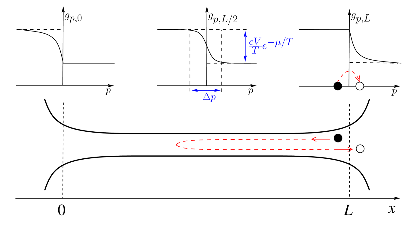
Figure 3: As one goes along the wire from the left lead to the right one, the distribution function of holes changes. The number of left-moving holes decreases as some of them turn around and start moving to the right.

At this point we can estimate the upper limit $l_{1}$ on the length of the wire $L$, to which the approach used here is applicable. In order to neglect the term $B(\partial/\partial p)[(p/2mt)\tilde{g}]$ in the right hand side of equation (22) we assumed $\Delta p\ll(mT)^{1/2}$. From Eq. (23) we see that this approximation fails when the length of the wire reaches the value

$$l_{1}\sim\frac{(mT^{3})^{1/2}}{B}\sim\left(\frac{\mu}{T}\right)^{1/2}l_{eee},$$ (24)

where we also used our earlier estimate (17) of $B$. As expected, $l_{1}\gg l_{0}$, see Eq. (14), i.e., the approach used in this section applies to a parametrically broad range of wire lengths.

To find the effect of three-particle scattering on the conductance of the wire we use the boundary conditions (20) to estimate

$$\left(\frac{\partial g_{p,x}}{\partial p}\right)_{p=0}\sim-\frac{1}{\Delta p}\frac{eV}{T}e^{-\mu/T}.$$

Substituting this estimate into Eq. (21), we obtain the correction to the conductance in the form

$$\delta G\sim-{2e^{2}\over h}\left({L\over l_{1}}\right)^{2/3}e^{-\mu/T}.$$ (25)

This correction should be compared with the result (6) of Lunde et al.lunde1 Both expressions are exponentially small and grow with the length of the wire, but correction (25) shows a slower growth, $\delta G\propto L^{2/3}$, rather than linear growth in Eq. (6). One can easily check that at the crossover, $L\sim l_{0}$, the results (6) and (25) are of the same order of magnitude.

II.2.2 Wires of length in the range $l_{1}\ll L\ll l_{\rm eq}$

As mentioned above, a hole near the bottom of the band performs a random walk in momentum space. In the case of wires longer than $l_{1}$ one needs to carefully consider the effect of the parabolic spectrum of the hole $-p^{2}/2m$. This spectrum plays the role of a potential barrier for the random walker, see Fig. 4. In order for the hole to backscatter, and thus change sign of its momentum, it has to overcome the barrier. The rate of such backscattering events is controlled by the height of the barrier measured from the Fermi level, and is exponentially small as $e^{-\mu/T}$. Evaluating the prefactor of backscattering rate is an interesting problem, similar to that of a Brownian particle escaping from a local minimum of the external potential. The general features of this problem are well understood.fpp In order to overcome the barrier the particle has to not just reach the top, but move beyond it far enough for the potential to drop below the maximum by more than the temperature $T$. Applied to a hole diffusing in momentum space, this means that the backscattering is controlled by the region of width $\Delta p\sim\sqrt{mT}$ around $p=0$.

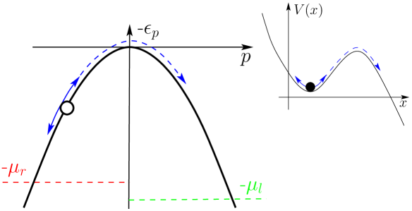
Figure 4: A hole with spectrum $-p^{2}/2m$ performs a random walk in momentum space in the presence of a barrier. Backscattering of a hole is analogous to a Brownian particle escaping from a local minimum of the potential, see inset.

In wires shorter than $l_{1}$ this process cannot fully develop because of the small time needed for the hole to traverse the wire, and one has to include into consideration the spatial dependence of the distribution function $g_{p,x}$. At $L\gg l_{1}$ the holes spend enough time inside the wire to fully complete the backscattering process. Therefore, away from the ends of the wire the distribution function no longer depends on position. As a result, the left-hand side of the kinetic equation (19) vanishes, and it can be rewritten in the form

$$\frac{\partial}{\partial p}\left(-\frac{p}{mT}\,g_{p}+\frac{\partial g_{p}}{\partial p}\right)=0.$$ (26)

To complete the mathematical formulation of the problem one has to impose the appropriate boundary conditions on the distribution function. Since equation (26) ignores the spatial dependence of the distribution function, we cannot reuse the boundary conditions (20). Instead we assume that the chemical potentials of the right- and left moving holes are established by the leads and do not vary along the wire:

$$g_{p}=\left\{\begin{array}[]{ll}e^{p^{2}/2mT}e^{-(\mu+eV)/T},&\text{for }p\gg\sqrt{mT},\\ e^{p^{2}/2mT}e^{-\mu/T},&\text{for }-p\gg\sqrt{mT}.\end{array}\right.$$ (27)

This assumption implies that the total number of backscattered holes is too small to affect the chemical potentials. This is justified by the fact that the backscattering rate is exponentially small. In wires of exponentially large length $L\gtrsim l_{\rm eq}$ this condition is violated. The latter regime will be discussed in Sec. III.

The solution of equation (26) with boundary conditions (27) is straightforward and gives

$$g_{p} = e^{p^{2}/2mT}e^{-\mu/T}$$ (28)

$$\times\left(1+\frac{e^{-eV/T}-1}{\sqrt{2\pi mT}}\int_{-\infty}^{p}e^{-{p^{\prime 2}}/2mT}dp^{\prime}\right).$$

This distribution function smoothly interpolates between the boundary conditions (27) imposed by the applied bias. As expected, the crossover occurs in a narrow region of width $\Delta p\sim\sqrt{mT}$ at the bottom of the band.

To linear order in $eV/T$ we find

$$\left(\frac{\partial g_{p}}{\partial p}\right)_{p=0}=-\frac{eV}{\sqrt{2\pi mT^{3}}}\,e^{-\mu/T},$$ (29)

resulting in the backscattering rate

$$\dot{N}^{R}=-\frac{eVBL}{h\sqrt{2\pi mT^{3}}}\,e^{-\mu/T},$$ (30)

see Eq. (21b). As a result, the correction to the conductance (21a) takes the form

$$\delta G=-{2e^{2}\over h}{L\over l_{1}}\,e^{-\mu/T},$$ (31)

where we have used the following precise definition

$$l_{1}=\frac{\sqrt{8\pi mT^{3}}}{B}$$ (32)

of the length $l_{1}$, consistent with our earlier estimate (24). It is worth mentioning that for wires of length $L\sim l_{1}$ the expressions (25) and (31) give the same estimate for $\delta G$.

Our result (31) has the form similar to the prediction (6) of Lunde et al.lunde1 for short wires, $L\ll l_{0}$. Both expressions for the correction to the conductance are exponentially small, but grow linearly with the length of the wire $L$. However, due to the sublinear growth (25) in the intermediate range of wire lengths $l_{0}\ll L\ll l_{1}$, the prefactor $l_{1}^{-1}$ in Eq. (31) is parametrically smaller than $l_{eee}^{-1}$ in Eq. (6), see (24).

The result (31) can be derived qualitatively, following arguments similar to the ones used in Sec II.1. There the change $\dot{N}^{R}$ in the number of right-moving electrons per unit time was estimated as the ratio of the number of holes likely to backscatter and the average time $\tau_{0}$ of such backscattering event, see Eq. (12). Compared to the case of very short wires considered in Sec II.1, for a hole to change direction, it must now cover a larger distance $(\Delta p)_{1}\sim\sqrt{mT}\gg(\Delta p)_{0}\sim T/v_{F}$ in momentum space set by the smearing of the discontinuity of the distribution function at the bottom of the band. The number of states available for the passage is thus larger by a factor $(\Delta p)_{1}/(\Delta p)_{0}\sim\sqrt{\mu/T}$ compared to the case of a very short wire, Sec II.1. On the other hand, even though the typical time between two three-particle collisions is still given by $\tau_{0}$, it now takes many such collisions for a hole to complete the backscattering process. Because the hole performs a random walk in momentum space, the time $\tau_{1}$ it takes to cover the longer distance $(\Delta p)_{1}$ can be estimated from $\tau_{1}/\tau_{0}\sim(\Delta p)_{1}^{2}/(\Delta p)_{0}^{2}\sim\mu/T$. Combining both effects we find that the correction to the conductance (31) should be smaller than (6) by a factor of $\sqrt{\mu/T}$, in agreement with Eq. (24).

III Conductance of long wires

In short quantum wires, the distribution function of electrons remains close to the unperturbed form (1) provided by the leads. The main change due to the processes of electron collisions occurs near the bottom of the band, with the discontinuity at $p=0$ being gradually smeared as the wire length $L$ increases. Because the discontinuity affects only electrons deep below the Fermi level, the effect of collisions is exponentially small. In particular, this enabled us to neglect the effect of collisions on the chemical potentials and assume that to first approximation the right- and left-moving electrons remain in equilibrium with the left and right leads, respectively.

A much more significant change occurs in long wires, $L\sim l_{\rm eq}\propto e^{\mu/T}$, for which the exponential suppression of the equilibration effects is compensated by a large system size. Once the length of the wire becomes exponentially large, the relaxation of the electron system becomes significant, and eventually, at $L\gg l_{\rm eq}$ the distribution function assumes the fully equilibrated form of Eq. (3). Unlike the relatively minor modification of the distribution function in short wires, the difference between the distributions (1) and (3) is not exponentially small and, more importantly, concentrated near the Fermi points, rather than at the bottom of the band. In this section we consider the conductance of the partially equilibrated wires, of length $L\sim l_{\rm eq}$. We start by discussing the form of the electron distribution in this regime.

III.1 Electron distribution function in the case of partial equilibration

Let us consider a segment of the wire, whose length $\Delta L$ is small compared to the equilibration length $l_{\rm eq}\propto e^{\mu/T}$. This condition implies that a typical electron with energy near the Fermi level passes through the segment without backscattering. On the other hand, $\Delta L$ is assumed to be sufficiently large for electrons to experience multiple three-particle collisions, which do not result in backscattering. Under these circumstances, the electron distribution function in the segment will achieve a state of partial equilibration, in which the numbers $N^{R}$ and $N^{L}$ of the right- and left-moving electrons are not changed by collisions. The form of this distribution can be obtained from a general statistical mechanics argument. The multiple collisions occurring in the system will maximize the entropy of the non-interacting electrons

$${\cal S}=-2\sum_{p}[f_{p}\ln f_{p}+(1-f_{p})\ln(1-f_{p})],$$ (33)

while preserving the total energy, momentum, $N^{R}$, and $N^{L}$, given by

$$E = 2\sum_{p}\epsilon_{p}f_{p},$$ (34a)

$$P = 2\sum_{p}pf_{p},$$ (34b)

$$N^{R} = 2\sum_{p>0}f_{p},$$ (34c)

$$N^{L} = 2\sum_{p<0}f_{p}.$$ (34d)

Subtracting from the functional (33) the expressions for the conserved quantities (34a)–(34d) with the Lagrange multipliers $\beta$, $-\beta u$, $-\beta\mu^{R}$, and $-\beta\mu^{L}$, respectively, and differentiating with respect to $f_{p}$, we find that the maximum of entropy is achieved for the distribution

$$f_{p}=\frac{\theta(p)}{e^{(\epsilon_{p}-up-\mu^{R})/{\cal T}}+1}+\frac{\theta(-p)}{e^{(\epsilon_{p}-up-\mu^{L})/{\cal T}}+1}.$$ (35)

Here ${\cal T}=1/\beta$ is the effective temperature, parameter $u$ has dimension of velocity and accounts for conservation of momentum in electron collisions, $\mu^{R}$ and $\mu^{L}$ are the chemical potentials of the right- and left-moving particles.

It is worth mentioning that the distribution (35) does not apply to particles near the bottom of the band, $p\sim\sqrt{mT}$. Indeed, for a hole near $p=0$ collisions with and without backscattering (i.e., the change of the sign of $p$) are roughly equally likely. Thus the above discussion is not applicable in this case. In order to find the form of the distribution function near the bottom of the band, one should perform an analysis similar to that of Sec. II.2.2. In particular, the exponentially small discontinuity of the distribution (35) at $p=0$ will be smeared. On the other hand, most quantities of interest are determined by the behavior of the distribution function near the Fermi level. For instance, using (35) we obtain the electric current in the form

$$I={2e\over h}\Delta\mu+enu,$$ (36)

up to corrections small as $e^{-\mu/T}$. Here $\Delta\mu=\mu^{R}-\mu^{L}$.

It is instructive to see how the distribution (35) interpolates between the regimes of no equilibration (1) and that of full equilibration (3). The unperturbed distribution (1) is obtained from (35) by setting $u=0$ and identifying the chemical potentials with those in the leads: $\mu^{R}=\mu_{l}$ and $\mu^{L}=\mu_{r}$. In this case $\Delta\mu=eV$, and Eq. (36) reproduces the Landauer formula. The fully equilibrated distribution (3) is obtained from (35) by setting $\Delta\mu=\mu^{R}-\mu^{L}=0$. In this case the electric current (36) is expressed as $I=enu$, which identifies parameter $u$ with the drift velocity $v_{d}$.

In the regime when the distribution function (35) differs from the limiting cases (1) and (3) it is convenient to quantify the degree of equilibration in the wire by the parameter

$$\eta={u\over v_{d}}.$$ (37)

The case of no equilibration corresponds to $\eta=0$ and that of full equilibration to $\eta=1$.

The meaning of the distribution function (35) can be further clarified by considering the Boltzmann equation (7). The scattering processes contributing into the collision integral (8) fall into two categories. The strongest processes preserve the numbers of the right- and left-moving electrons, whereas the ones resulting in backscattering are exponentially weak, as discussed by Lunde et al.lunde1 and also above in Sec. II. Let us approximate the collision integral (8) by neglecting the weak backscattering processes. Then, by substituting the distribution (35) into the right-hand side of Eq. (8), one easily sees that each term in the sum vanishes. Thus the distribution (35) solves the Boltzmann equation (7) in this approximation. Furthermore, in the absence of backscattering the solution (35) applies for any choice of parameters ${\cal T}$, $u$, $\mu^{R}$, and $\mu^{L}$, and in particular, for any degree of equilibration $\eta$. The value of $\eta$ is ultimately determined by the exponentially weak backscattering processes and the length of the wire.

III.2 Conservation laws

Conductance of a long quantum wire, in which the electron distribution function is fully equilibrated, was studied in Ref. [jerome3, ], where a power-law correction to the quantized conductance was obtained, Eq. (4). The derivation of this result was based on an analysis of conservation laws for the number of electrons, energy, and momentum satisfied in electron collisions. Here we perform a similar analysis for a partially equilibrated wire.

Conservation of the total number of particles $N$ implies that in a steady state the particle current $j(x)$ is uniform along the wire. Correspondingly, we infer from the conservation of total momentum $P$ and total energy $E$ that in the steady state a constant momentum current $j_{P}$ and a constant energy current $j_{E}$ flow through the system. In the following it will be convenient to express these currents as the sum of the individual contributions from left- and right-moving electrons, e.g. $j=j^{R}+j^{L}$, thus introducing

$$j^{R/L}(x) = \int_{-\infty}^{\infty}{dp\over h}\theta(\pm p)v_{p}f_{p,x},$$ (38a)

$$j_{P}^{R/L}(x) = \int_{-\infty}^{\infty}{dp\over h}\theta(\pm p)v_{p}pf_{p,},$$ (38b)

$$j_{E}^{R/L}(x) = \int_{-\infty}^{\infty}{dp\over h}\theta(\pm p)v_{p}\epsilon_{p}f_{p,x}.$$ (38c)

Here $v_{p}=p/m$ is the electron velocity, the positive sign in the step function corresponds to right-movers, while the negative one to left-movers.

Near the ends of the wire, the distribution function of incoming electrons is controlled by the leads. Close to the left lead, the distribution $f^{R}$ of right-moving electrons thus assumes the form of the first term in Eq. (1), and similarly, close to the right lead, the left-movers’ distribution $f^{L}$ is given by the second term in Eq. (1). This allows us to readily calculate, for example, the current $j^{R}(l)$ of right-moving electrons near the left end of the wire. Unlike the total current $j$, the current $j^{R}(x)$ is not uniform throughout the system, since the equilibration processes ensure the conversion of right-moving electrons into left-moving ones. From conservation of the number of particles it follows that the total number of right-moving electrons changing direction per unit time equals the difference between their outgoing and incoming flows at the right and left leads

$$\dot{N}^{R}=j^{R}(r)-j^{R}(l).$$ (39)

A calculation of $j^{R}(r)$ requires the knowledge of the distribution of right-moving electrons at the right end of the wire. As the latter is unknown, we proceed by expressing $j^{R}(r)$ in terms of the total particle current $j$ and the incoming flow of left-movers supplied by the right lead

$$j^{R}(r)=j-j^{L}(r),$$ (40)

where $j^{L}(r)$ can now be determined from the known electron distribution in the right lead. Combining Eqs. (39) and (40) we can relate $\dot{N}^{R}$ to the total incoming flow of particles as

$$j^{R}(l)+j^{L}(r)=j-\dot{N}^{R}.$$ (41)

Using the lead distribution function (1) the left-hand side of (41) is readily calculated, and takes the form $G_{0}V/e$, with the conductance $G_{0}$ defined by Eq. (2). Noticing that the electric current $I=ej$, we then recover Eq. (5). For the purposes of this section we do not need to keep the exponentially small corrections to $G_{0}$, and upon substitution $G_{0}=2e^{2}/h$ we are left with the relation

$${2e\over h}V=j-\dot{N}^{R},$$ (42)

between voltage, current, and the rate of change of the number of right moving electrons due to collisions.

Let us now analyze the consequences of energy conservation in electron-electron collisions. Repeating the above steps for the energy current $j_{E}$, we arrive at an expression

$$j_{E}^{R}(l)+j_{E}^{L}(r)=j_{E}-\dot{E}^{R},$$ (43)

analogous to Eq. (41). Here $\dot{E}^{R}$ is the rate of change of the energy of right-movers.

The conservation of the number of electrons and energy ensure that the currents $j$ and $j_{E}$ are constant along the wire. It is convenient to combine them into the heat current

$$j_{Q}=j_{E}-\mu j,$$ (44)

which is consequently also independent of position.footnote Combining Eq. (43) and (41) we find

$$j_{Q}^{R}(l)+j_{Q}^{L}(r)=j_{Q}-\dot{Q}^{R},$$ (45)

where

$$\dot{Q}^{R}=\dot{E}^{R}-\mu\dot{N}^{R}$$ (46)

is the heat transferred into the right-moving subsystem by electron collisions.

The left-hand side of Eq. (45) is the heat current in a non-interacting quantum wire. Direct calculation shows that it is exponentially small (see also the discussion in the beginning of Sec. IV), and for our purposes here can be assumed to vanish. We therefore conclude

$$j_{Q}=\dot{Q}^{R}.$$ (47)

Since the heat current $j_{Q}$ does not depend on position, it can be calculated at any point in the wire. In the regions not too close to the leads the distribution function is expected to have the partially equilibrated form (35). Then, using the expressions (38a) and (38c) for $j$ and $j_{E}$, we obtain

$$j_{Q}={\pi^{2}\over 6}{T^{2}\over\mu}nu$$ (48)

to leading order in $T/\mu$. As expected, in the absence of equilibration, $u=0$, the heat current vanishes.

In Sec. III.1 we introduced the distribution function (35) by discussing a short segment of the wire. The four parameters of this distribution ${\cal T}$, $u$, $\mu^{R}$, and $\mu^{L}$ may, in principle, vary along the wire. The independence of heat current (48) on position then shows that the velocity $u$ and, therefore, the degree of equilibration $\eta$ are constant along the wire. Furthermore, since the electric current (36) and $u$ are constant along the wire, one concludes that the difference of the chemical potentials $\Delta\mu=\mu^{R}-\mu^{L}$ is constant as well. The only two parameters of the distribution (35) that can vary along the wire are the temperature ${\cal T}$ and the average chemical potential $(\mu^{R}+\mu^{L})/2$. Their dependences on position are discussed in Appendix C.

III.3 Relation between the degree of equilibration $\eta$ and the conductance of the wire

To make further progress we elaborate on the relationship between the rates $\dot{N}^{R}$ and $\dot{E}^{R}$, whose explicit forms depend on the details of the equilibration mechanism. As we discussed in Sec. III.1, in the absence of scattering processes which change the number of left- and right-moving electrons, the distribution (35) is unaffected by electron-electron collisions, i.e., the collision integral (8) vanishes. In particular, for $u=0$ the unperturbed distribution (1) supplied by the leads would retain its form in the wire. The backscattering processes, which by definition contribute to $\dot{N}^{R}$, also change the energy of the subsystem of right-moving electrons, resulting in a non-vanishing $\dot{E}^{R}$. Because both rates are caused by the same backscattering processes, one expects to find a relation between $\dot{N}^{R}$ and $\dot{E}^{R}$. Here we establish such a relation with the help of conservation laws. An alternative and more formal derivation can be found in Appendix D.

The backscattering processes transform the unperturbed distribution (1) to the partially equilibrated form (35) with non-vanishing $u$. The two distributions differ most prominently at energies within $\sim T$ of the Fermi level. One can thus assume that all the right-moving electrons contributing to $\dot{N}^{R}$ are removed from the vicinity of the right Fermi point and placed to the vicinity of the left one. Each such transfer reduces the momentum of the system by $2p_{F}$. Since the electron-electron collisions conserve momentum, a number of other electrons have to be scattered in the vicinities of the two Fermi points, see Fig. 5. In the special case of three particle collisions, the transfer of electron from the right Fermi point to the left one is accomplished in a number of small steps with momentum change $\delta p\sim T/v_{F}$, and at each step one additional electron is scattered near each of the two Fermi points, see Fig. 2(b).

As a result of the rearrangement of electrons near the two Fermi points, the momentum change $2p_{F}$ of the backscattered electrons is distributed between the remaining right- and left-moving electrons, i.e., $\Delta p^{R}+\Delta p^{L}=2p_{F}$. Thus the energy of the remaining right-movers increases by $\Delta Q^{R}=v_{F}\Delta p^{R}$ whereas that of the left movers decreases, $\Delta Q^{L}=-v_{F}\Delta p^{L}$. Then, the conservation of energy requires $\Delta p^{R}=\Delta p^{L}=p_{F}$. In the end, the energy balance for the right-moving electrons consists of a loss of $\epsilon_{F}$ due to removal of one particle from the Fermi level and a gain of $\Delta Q^{R}=v_{F}p_{F}=2\epsilon_{F}$ due to the redistribution of momentum. As a result, for every right-moving electron that changes direction, $\Delta N^{R}=-1$, the right-movers’ energy increases by an amount $\Delta E^{R}=\epsilon_{F}$. It is easy to check that the difference between the chemical potential $\mu$ and the Fermi energy $\epsilon_{F}$ is irrelevant for our discussion, so we conclude

$$\dot{E}^{R}=-\mu\dot{N}^{R}.$$ (49)

It is important to point out that this result is independent of a specific equilibration mechanism, or the degree to which equilibration has occurred.

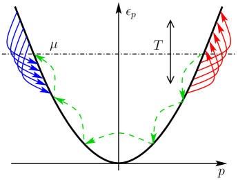
Figure 5: Sequence of elementary scattering events leading to the transfer of one electron from the right to the left Fermi point. Conservation of momentum leads to the heating of the right-moving electrons and cooling of the left-moving ones.

The result (49) can be also expressed in the form

$$\dot{Q}^{R}=-2\mu\dot{N}^{R},$$ (50)

cf. Eq. (46), which expresses the simple fact that when a right-moving electron is moved to the left Fermi point, the remaining right-movers gain energy, see Fig. 5. Combining this expression with Eqs. (47) and (48), we obtain

$$\dot{N}^{R}=-r_{0}nu,$$ (51)

where the dimensionless parameter $r_{0}$ is defined as

$$r_{0}={\pi^{2}\over 12}\left({T\over\mu}\right)^{2}.$$ (52)

Noticing that by definition of the degree of equilibration (37) $nu=\eta nv_{d}=\eta j$ and using the conservation of the particle number in electron collisions, Eq. (42), we find a linear relation between the applied bias and the electric current flowing through the wire. We can thus readily extract the expression for the conductance in partially equilibrated wires

$$G={2e^{2}\over h}\left[1-\eta{\pi^{2}\over 12}\left({T\over\mu}\right)^{2}\right],$$ (53)

where we discarded higher-order corrections in $(T/\mu)^{2}$.

The result (53) reaffirms that at finite temperature the processes of equilibration of the electron distribution function lead to a deviation of the conductance from its quantized value $2e^{2}/h$. In a fully equilibrated wire $\eta\to 1$, and this correction saturates at a value that does not depend on the details of the electron-electron interaction, reproducing our earlier result (4). The correction to the conductance in this situation is quadratic in temperature $\delta G\propto\left(T/\mu\right)^{2}$, in contrast with the results for the short wire, where $\delta G\sim e^{-\mu/T}$.

We obtained the expression (53) for the conductance of the wire by taking advantage of the conservation laws for the electron-electron collisions as well as the basic properties of the non-interacting leads the wire is connected to. Although the expression (53) is thus very general, it does not fully determine the conductance of the wire, as the parameter $\eta$ cannot be obtained in this approach, with the exception of special cases of non-interacting electrons, $\eta=0$, and a very long wire, $\eta=1$. To find $\eta$ and, therefore, the conductance of the wire, for arbitrary wire length, one needs to consider a specific model of electron-electron interactions. We now turn to such a calculation for the most relevant case of relaxation via three-particle collisions.

III.4 Partially equilibrated wires and equilibration length

Our expression (53) for the conductance of partially equilibrated wires relied on the relation (51) between the rate $\dot{N}^{R}$ of backscattering of right-moving electrons in the wire and the parameter $u$ of the distribution function (35). Another relation between $\dot{N}^{R}$ and the distribution function can be found by considering the microscopic mechanism of such backscattering, using the approach of Sec. II.2.2. Comparison of the two expressions will enable us to determine the degree of equilibration $\eta$ for wires of arbitrary length.

The form of the electron distribution in a partially equilibrated state (35) is controlled by four parameters, namely, the temperature ${\cal T}$, average chemical potential $\mu=(\mu^{R}+\mu^{L})/2$, difference of the chemical potentials $\Delta\mu=\mu^{R}-\mu^{L}$, and the velocity $u$. In the absence of bias $V$ applied to the wire, the temperature ${\cal T}$ and chemical potential $\mu$ are equal to those in the leads, whereas $\Delta\mu$ and $u$ vanish. As a result the distribution (35) reproduces the equilibrium Fermi-Dirac distribution, and clearly $\dot{N}^{R}=0$. Our goal is to find $\dot{N}^{R}$ to linear order in $V$.

Applied bias affects the four parameters of the distribution (35) differently. As we discussed at the end of Sec. III.2, the temperature ${\cal T}$ and chemical potential $\mu$ acquire position dependence, whereas $\Delta\mu$ and $u$ no longer vanish, but remain constant along the wire. Thus, to linear order in $V$ one expects to find for the rate $\dot{n}^{R}$ of backscattering per unit length of the wire

$$\frac{\dot{N}^{R}}{L}=\gamma_{1}\Delta\mu+\gamma_{2}u+\gamma_{3}\,\partial_{x}{\cal T}+\gamma_{4}\partial_{x}\mu.$$ (54)

Because the gradients $\partial_{x}{\cal T}$ and $\partial_{x}\mu$ are caused by bias applied to a long wire, they are not only proportional to $V$, but also scale as $1/L$ (see also Appendix C). Thus for the exponentially long wires considered here, $L\sim l_{\rm eq}$, effect of the gradients of ${\cal T}$ and $\mu$ can be neglected. It is also clear that $\gamma_{2}=0$. Indeed, at $\Delta\mu=0$ the distribution takes the fully equilibrated form (3), for which no relaxation takes place, and $\dot{N}^{R}=0$ for any $u$. We thus conclude that the backscattering rate $\dot{n}^{R}$ can be found for the simplest case of small $\Delta\mu$, vanishing $u$, and unperturbed (position-independent) values of the temperature ${\cal T}=T$ and average chemical potential $\mu$.

The resulting problem is equivalent to the one considered in Sec. II.2.2. The only difference is that because the length of the wire was assumed to be short, $L\ll l_{\rm eq}$, the parameter $\Delta\mu$ coincided with $eV$. Thus replacing $eV\to\Delta\mu$ in Eq. (30) we find

$$\dot{N}^{R}=-r_{1}\frac{2\Delta\mu}{h}.$$ (55)

Here the dimensionless parameter $r_{1}$ is defined as

$$r_{1}=\frac{L}{l_{1}e^{\mu/T}},$$ (56)

and the length $l_{1}$ is given by Eq. (32).

Our expression (55) and the earlier result (51) relate $\dot{N}^{R}$ to two different parameters of the distribution function (35), namely, $\Delta\mu$ and $u$. Both of these parameters affect the electric current in the wire and can be expressed in terms of the drift velocity $v_{d}=I/ne$ and the degree of equilibration $\eta$. Indeed, according to the definition (37) of $\eta$ and the expression (36) for the current, we have

$$nu=\eta\,nv_{d},\quad\frac{2\Delta\mu}{h}=(1-\eta)nv_{d}.$$ (57)

Using these expressions to compare Eqs. (51) and (55), we readily find the following expression for the parameter $\eta$

$$\eta=\frac{r_{1}}{r_{0}+r_{1}}=\frac{L}{l_{\rm eq}+L},$$ (58)

where we have introduced the equilibration length

$$l_{\rm eq}=r_{0}l_{1}e^{\mu/T}.$$ (59)

As expected, parameter $\eta$ grows with the length of the wire from 0 to 1. Because the backscattering process involves rare holes at the bottom of the band, the equilibration length (59) at which the crossover occurs is exponentially long at low temperatures.

Substituting Eq. (58) into (53) we find the following expression for the conductance of a quantum wire

$$G={2e^{2}\over h}\left[1-{\pi^{2}\over 12}\left({T\over\mu}\right)^{2}\frac{L}{l_{\rm eq}+L}\right],$$ (60)

valid for $L\gg l_{1}$. At $L\to\infty$ it recovers the long wire limit (4), while at $l_{1}\ll L\ll l_{\rm eq}$ it agrees with our earlier result (31).

IV Thermoelectric properties of long wires

We now turn to a situation in which the leads are not only biased by a finite voltage $V$ but also exposed to a temperature drop $\Delta T$. More specifically, we assume that the leads supply the wire with the following electron distribution

$$f_{p}^{(0)}=\frac{\theta(p)}{e^{(\epsilon_{p}-\mu-eV)/(T+\Delta T)}+1}+\frac{\theta(-p)}{e^{(\epsilon_{p}-\mu)/T}+1}.$$ (61)

Our goal is to find the thermopower $S$, Peltier coefficient $\Pi$, and the thermal conductance $K$ of the quantum wire. These transport coefficients are defined by the following linear response relations

$$V = -S\Delta T\big{|}_{I=0},$$ (62)

$$j_{Q} = \Pi I\big{|}_{\Delta T=0},$$ (63)

$$j_{Q} = K\Delta T\big{|}_{I=0}.$$ (64)

The thermopower and Peltier coefficient are not independent properties of the system; they are connected by an Onsager relation $\Pi=ST$.

In the absence of interactions, electron distribution in the wire is given by Eq. (61), and its transport coefficients are easily understood. For instance, the thermopower and Peltier coefficient are given by

$$\Pi=ST=\frac{1}{e}[\mu e^{-\mu/T}+T(1+e^{-\mu/T})\ln(1+e^{-\mu/T})].$$ (65)

At low temperature $T\ll\mu$, the expression (65) is exponentially small, $\Pi\sim(\mu/e)\,e^{-\mu/T}$. The reason is that contributions to the heat current from electrons with energies $\mu+\xi$ and $\mu-\xi$ cancel each other, and the only reason $\Pi$ does not vanish completely is the absence of electronic states below the bottom of the band. In this paper we are not interested in such exponentially small results, unless the smallness can be compensated by a long length of the wire. Thus to first approximation the thermopower and Peltier coefficient of a non-interacting quantum wire vanish. The latter conclusion can be easily obtained from the so-called Cutler-Mott formulamott

$$S=\frac{\pi^{2}T}{3e}\frac{d\ln G}{d\epsilon_{F}},$$ (66)

generally applicable to systems of non-interacting electrons at $T\ll\epsilon_{F}$. Considering that the conductance $G=2e^{2}/h$ does not depend on the Fermi energy $\epsilon_{F}$, one easily concludes that $S=0$.

To the same accuracy, i.e., neglecting corrections small as $e^{-\mu/T}$, the thermal conductance of a non-interacting quantum wire is

$$K=\frac{2\pi^{2}}{3h}\,T.$$ (67)

This expression can be derived by straightforward calculation of the heat current for the electron distribution (61) with $V=0$. Alternatively, one can obtain (67) from the Wiedemann-Franz law

$$K=\frac{\pi^{2}}{3e^{2}}\,TG,$$ (68)

by substituting the quantized conductance $G=2e^{2}/h$.

It is important to note that both the Cutler-Mott formula (66) and Wiedemann-Franz law (68) are not generally applicable to systems where inelastic scattering of electrons plays an important role. Thus one cannot expect to find the transport coefficients $S$, $\Pi$, and $K$ in long quantum wires by combining these relations with the expression (60) for the conductance. Below we find the transport coefficients of a long wire, whose length $L\sim l_{\rm eq}\propto e^{\mu/T}$. We will see that in such wires the thermopower and Peltier coefficient are no longer exponentially small, whereas the thermal conductance $K$ is suppressed at $L\to\infty$.

Unlike the thermopower and thermal conductance, the Peltier coefficient $\Pi$ is defined in a system to which no temperature bias is applied, see Eq. (63). One can therefore obtain $\Pi$ using the results of Sec. III. In particular, we saw that in a long wire the heat current is determined by the parameter $u$ of the distribution function, see Eq. (48). The value of $u$ depends on the length of the wire via expressions (57) and (58). Combining these results we find the heat current in the form

$$j_{Q}=\frac{\pi^{2}}{6}\,\frac{T^{2}}{\mu}\,\frac{L}{l_{\rm eq}+L}\,nv_{d}.$$ (69)

The ratio of $j_{Q}$ and the electric current $I=env_{d}$ gives the Peltier coefficient

$$\Pi=\frac{\pi^{2}}{6e}\,\frac{T^{2}}{\mu}\,\frac{L}{l_{\rm eq}+L}.$$ (70)

Similar to our main result (60) for the conductance, Eq. (70) is applicable at $L\gg l_{1}$. It shows how $\Pi$ grows from exponentially small values at $L\ll l_{\rm eq}$ to $\pi^{2}T^{2}/6e\mu$ at $L\to\infty$.

The thermopower and thermal conductance are defined in a system with a small temperature bias $\Delta T$. To find these transport coefficients we revise our analysis of the conservation laws (41) and (45) to add finite $\Delta T$. The left-hand side of Eq. (41) represents the particle current $j=I/e$ in the wire with electron distribution (61). As we saw above, the thermopower of such a wire (65) is exponentially small, and thus the effect of temperature bias on the current $j$ is negligible. We thus have $j=2eV/h$ and recover Eq. (42).

The left-hand side of Eq. (45) is the heat current in a wire with electron distribution (61), which does not vanish at $\Delta T\neq 0$. It is determined by the thermal conductance (67) of a non-interacting wire. Thus instead of Eq. (47) we obtain

$$\frac{2\pi^{2}}{3h}\,T\Delta T=j_{Q}-\dot{Q}^{R}.$$ (71)

The right-hand sides of equations (42) and (71) are not directly related to the voltage and temperature bias of the wire, but are determined by parameters $\Delta\mu$ and $u$ of the partially equilibrated distribution (35). Indeed, the currents $j$ and $j_{Q}$ do not depend on position, and can be calculated for the internal region of the wire using Eqs. (36) and (48). The backscattering of the right-moving electrons predominantly happens inside the wire, at distances over $l_{1}$ from the leads, where the partially equilibrated distribution (35) is established. Thus we can express $\dot{N}^{R}$ and $\dot{Q}^{R}$ in terms of $\Delta\mu$ using the results (55) and (50) of Sec. III. As a result, we obtain the following two linear equations upon the parameters $\Delta\mu$ and $u$,

$$(1+r_{1})\frac{2\Delta\mu}{h}+nu = \frac{2eV}{h},$$ (72a)

$$-r_{1}\frac{2\Delta\mu}{h}+r_{0}nu = \frac{\pi^{2}}{3h}\,\frac{T}{\mu}\Delta T.$$ (72b)

The system of equations (72) can be easily solved. Then, substituting the resulting $\Delta\mu(V,\Delta T)$ and $u(V,\Delta T)$ into Eqs. (36) and (48), one finds the electric current $I$ and heat current $j_{Q}$.

On the other hand, it is easier to find the thermopower $S$ and thermal conductance $K$ by noticing that their definitions (62) and (64) assume the condition of zero current $I$. Then, from Eq. (36) we immediately find $\frac{2\Delta\mu}{h}=-nu$ and equations (72) reduce to

$$-r_{1}nu = \frac{2eV}{h},$$ (73a)

$$(r_{1}+r_{0})nu = \frac{\pi^{2}}{3h}\,\frac{T}{\mu}\Delta T.$$ (73b)

Excluding the unknown parameter $u$, we find the linear relation (62) between $V$ and $\Delta T$ with

$$S=\frac{\pi^{2}}{6e}\,\frac{T}{\mu}\,\frac{L}{l_{\rm eq}+L}.$$ (74)

Predictably, the thermopower (74) and the Peltier coefficient (70) satisfy the Onsager relation $\Pi=ST$.

Furthermore, using Eq. (73b) we express the heat current (48) in terms of $\Delta T$ as

$$j_{Q}=\frac{2\pi^{2}T}{3h}\,\frac{r_{0}}{r_{1}+r_{0}}\Delta T.$$ (75)

Thus the thermal conductance takes the form

$$K=\frac{2\pi^{2}T}{3h}\,\frac{l_{\rm eq}}{l_{\rm eq}+L}.$$ (76)

At $L\ll l_{\rm eq}$, Eq. (76) recovers the result (67) for noninteracting wires, but as the length of the wire grows, $K$ is suppressed as $1/L$.

The fact that the thermal conductance $K$ vanishes at $L\to\infty$ can be understood as follows. In an infinitely long wire the distribution function of electrons reaches the fully equilibrated form (3) controlled by three parameters, $T$, $\mu$, and the drift velocity $v_{d}$. The thermal conductance is defined under the condition that the electric current $I=env_{d}$ vanishes, see Eq. (64). Thus $v_{d}=0$ and the distribution (3) takes the form of the standard Fermi-Dirac distribution. Due to its symmetry $p\to-p$, the heat current $j_{Q}$ vanishes, regardless of the temperature bias $\Delta T$ applied to the wire. One therefore finds that in an infinitely long wire $K=0$.

The thermoelectric properties of a device are sometimes summarized in the form of the dimensionless figure of merit defined as

$$ZT={GS^{2}T\over K}.$$ (77)

The figure of merit measures the efficiency of thermoelectric refrigerators. As $ZT$ diverges, the device attains Carnot efficiency. For a material to be a good thermoelectric cooler, it must have a high value for $ZT$ and a typical figure of merit $ZT\simeq 3$ would make solid-state home refrigerators economically competitive with compressor-based refrigerators.mahan However, in many materials the figure of merit is limited by the Wiedemann-Franz law, and remains near 1.

Substituting our results (74) and (76) for a long wire and neglecting a small correction to the quantized conductance, we find

$$ZT\simeq\frac{\pi^{2}}{12}\left(\frac{T}{\mu}\right)^{2}\frac{L^{2}}{l_{\rm eq}(l_{\rm eq}+L)}.$$ (78)

In short wires the thermopower is small, resulting in a small $ZT$. On the other hand, the thermal conductance $K$ is strongly suppressed in long wires, giving rise to infinite figure of merit at $L\to\infty$.

V Discussion

In this paper we studied the transport properties of a partially equilibrated quantum wire. In one-dimensional systems, equilibration of weakly interacting electrons is strongly suppressed at low temperatures, and the resulting equilibration length $l_{\rm eq}$ is exponentially large, Eq. (59). Our main result is the expression (60) for the conductance of a wire whose length $L$ exceeds the length scale $l_{1}$ given by Eq. (32). Because the scale $l_{1}$ is only power-law large at low temperature, the expression (60) describes the full crossover behavior of conductance between the regimes of negligible and full equilibration. We have also been able to establish a connection between our result (60) and the expression (6) for the correction to the conductance of a short wire obtained by Lunde et al.lunde1 . Similar to Eq. (6), our result (60) is exponentially suppressed at small $L$ and grows linearly with $L$. However the prefactors are parametrically different. This mismatch is resolved by noticing that Eq. (6) is valid at $L\ll l_{0}$, where the length $l_{0}$ defined by Eq. (14) is short compared to $l_{1}$. In the regime of intermediate wire lengths, $l_{0}\ll L\ll l_{1}$, the correction to the conductance (25) scales with the length as $L^{2/3}$. A summary of our results for the conductance of a quantum wire as a function of its length is presented in Fig. 6.

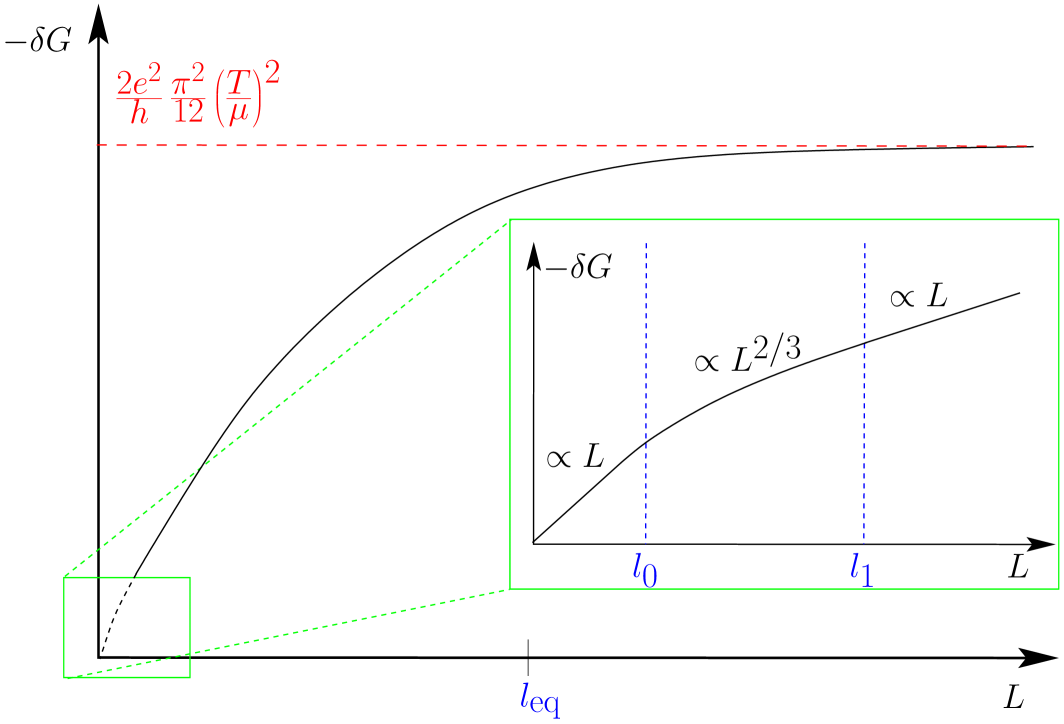
Figure 6: Correction to the conductance of a quantum wire as a function of its length. For wires longer than the scale $l_{1}$ the conductance is given by Eq. (60). The behavior of the conductance in the regions $L\ll l_{0}$ and $l_{0}\ll L\ll l_{1}$ is given by Eqs. (6) and (25), respectively.

In addition to conductance, we studied thermoelectric effects in partially equilibrated wires, limiting ourselves to the most interesting regime $L\gg l_{1}$. The equilibration of the electron system has a dramatic effect on the thermopower and thermal conductance of the wire. As the length of the wire increases, the thermopower increases dramatically, from exponentially small values at $L\ll l_{\rm eq}$ to $S\sim T/e\mu$ at $L\gg l_{\rm eq}$, see Eq. (74). Conversely, the thermal conductance of the wire decreases due to the equilibration of the electron system in the wire from the Wiedemann-Franz value $K=2\pi^{2}T/3h$ to zero, Eq. (76). As a result, at $L\gg l_{\rm eq}$ the quantum wire becomes a perfect thermoelectric refrigerator.

In this paper we accounted for the effect of electron-electron interactions but neglected the electron-phonon scattering, which may also affect the electron distribution function. In GaAs quantum wires the phonons are three-dimensional and in equilibrium with the rest of the system. Scattering of electrons by phonons should therefore have the effect of equilibrating them in the stationary reference frame, thereby reducing the degree of equilibration $\eta$. We leave the detailed study of the effect of phonon coupling to future work and limit our discussion here to a few qualitative remarks. The reason the electron-phonon coupling is typically neglected compared to electron-electron interactions is that respective coupling constant is much smaller for the phonons. On the other hand, we do not expect the effect of phonons on the electron distribution function to be exponentially suppressed as $e^{-\mu/T}$. Thus we expect that coupling to the phonons to be negligible only at not too low temperatures.

Another effect neglected in this paper is the possible presence of slight long-range inhomogeneities in the wire, which would typically be caused by the presence of remote impurities in the GaAs heterostructure. The effect of such inhomogeneities on the conductance was studied earlierjerome1 ; jerome2 under the assumption of full equilibration of the electron system. On the other hand, the inhomogeneities themselves resist the equilibration process, and we expect an interesting interplay of these effects in the case of a partially equilibrated wire. We leave such a study to future work.

Acknowledgements

We are grateful to B. L. Altshuler, A. V. Andreev, and L. I. Glazman for helpful discussions. This work was supported by the U.S. Department of Energy, Office of Science, under Contract No. DE-AC02-06CH11357, and through SFB/TR 12 of the Deutsche Forschungsgemeinschaft (DFG), the Center for Nanoscience (CeNS) Munich, and the German Excellence Initiative via the Nanosystems Initiative Munich (NIM).

Appendix A Screened Coulomb interaction

Let us consider the Coulomb interaction between electrons screened by a nearby gate, which we model by a conducting plane at a distance $d$ from the wire. In this case, the electron-electron interaction takes the form

$$V(x)={e^{2}\over\epsilon}\left({1\over|x|}-{1\over\sqrt{x^{2}+(2d)^{2}}}\right).$$ (79)

The diverging short-range behavior of this potential needs to be regularized in order to evaluate the small-momentum Fourier components $V_{q}$. To this end, we introduce the small width $w$ of the quantum wire, $w\ll d$. Then the homogeneous component $V_{0}$ of the interaction potential takes the form

$$V_{0}={2e^{2}\over\epsilon}\ln\left(\frac{d}{w}\right).$$ (80)

For small wave vectors $q\ll 1/d$, the Fourier transformed potential $V_{q}$ departs from the homogeneous component $V_{0}$ by an amount

$$V_{q}-V_{0} ={e^{2}\over\epsilon}\int dx\left[\cos(qx)-1\right]\left({1\over|x|}-{1\over\sqrt{x^{2}+(2d)^{2}}}\right)$$

$$\simeq-{2e^{2}\over\epsilon}d^{2}q^{2}\ln\left(\frac{1}{|q|d}\right).$$ (81)

It then follows that the small-$q$ behavior of the Fourier-transformed potential is given by

$$V_{q}=V_{0}\left[1-q^{2}d^{2}\frac{\ln(1/|q|d)}{\ln(d/w)}\right].$$ (82)

This expression contains an extra logarithmic-in-$q$ factor compared to the expression introduced by Lunde et al.,lunde1

$$V_{q}=V_{0}\left[1-\frac{q^{2}}{q_{0}^{2}}\right].$$ (83)

However, as argued in the text, the typical scattering processes studied here only involve small momentum exchanges, of the order $\hbar q\sim T/{v_{F}}$, so that the expression (82) for $V_{q}$ reduces to the one of Eq. (83) with

$$q_{0}=\frac{1}{d}\left(\frac{\ln(\hbar v_{F}/Td)}{\ln(d/w)}\right)^{1/2}.$$ (84)

The model introduced in Eq. (79), therefore merely amounts to an extra logarithmic temperature dependence in the length $l_{eee}$, Eq. (11).

Appendix B Fokker-Planck equation for 3-particle collisions

In this appendix we discuss the Fokker-Planck approximation and calculate the coefficients for the interaction potential used by Lunde et al. lunde1 as well as the screened and unscreened Coulomb interaction.

B.1 Fokker-Planck approximation

We start out from the collision integral (8) for the three-particle scattering process. We discussed in section II that the only contributions relevant to transport result from collisions involving two pairs of incoming and outgoing states in the vicinity of the right and left Fermi-points, and one pair of incoming and outgoing states at the bottom of the band, see Fig. 2b. Let $p_{1}$ and $p^{\prime}_{1}$ be the momenta near the bottom of the band, $p_{2}$ and $p^{\prime}_{2}$ the ones near the left Fermi point, while $p_{3}$ and $p^{\prime}_{3}$ are taken near the right Fermi point. Unprimed momenta correspond to incoming states whereas primed ones are associated with outgoing states. We introduce the hole distribution $g_{p_{i}}=1-f_{p_{i}}$ and the collision integral of holes $I_{p,x}[g]=-I_{p,x}[f]$, which using Eq. (8), can be recast as

$$I_{p_{1},x}[g] =\sum_{p^{\prime}_{1}}\left[W(p_{1},p^{\prime}_{1})g_{p^{\prime}_{1}}-W(p^{\prime}_{1},p_{1})g_{p_{1}}\right],$$ (85)

where

$$W(p_{1},p^{\prime}_{1}) =48\sum_{\begin{subarray}{c}p_{2},p_{3}\\ p^{\prime}_{2},p^{\prime}_{3}\end{subarray}}W_{123;1^{\prime}2^{\prime}3^{\prime}}g_{2^{\prime}}g_{3^{\prime}}f_{1}f_{2}f_{3},$$ (86)

$$W(p^{\prime}_{1},p_{1}) =48\sum_{\begin{subarray}{c}p_{2},p_{3}\\ p^{\prime}_{2},p^{\prime}_{3}\end{subarray}}W_{123;1^{\prime}2^{\prime}3^{\prime}}g_{2}g_{3}f_{1^{\prime}}f_{2^{\prime}}f_{3^{\prime}}.$$ (87)

$W(p_{1},p^{\prime}_{1})$ is the rate for a transition in which a hole scatters from some state $p^{\prime}_{1}$ into $p_{1}$, while $W(p^{\prime}_{1},p_{1})$ denotes the corresponding transition rate for the inverse process. Here and in what follows, all momentum summations are restricted to the ranges discussed above. This restriction results in a combinatorial factor of 12 in Eqs. (86) and (87). The remaining factor of 4 originates from the spin summations as we anticipated that the main contribution to the 3-particle scattering rate $w_{123;1^{\prime}2^{\prime}3^{\prime}}$ of Eq. (8) takes the form $\delta_{\sigma_{1}\sigma_{1^{\prime}}}\delta_{\sigma_{2}\sigma_{2^{\prime}}}\delta_{\sigma_{3}\sigma_{3^{\prime}}}W_{123;1^{\prime}2^{\prime}3^{\prime}}$, with a spin-independent $W_{123;1^{\prime}2^{\prime}3^{\prime}}$. This simplification is only valid in the limit of small momentum exchanges, and can be performed here since for the Coulomb interaction $V_{0}\gg V_{k_{F}}$. Since $p_{1}$ and $p^{\prime}_{1}$ lie near the bottom of the band, the distribution functions $g_{p_{1}}$ and $g_{p^{\prime}_{1}}$ are exponentially small, and so is the collision integral of holes (85). It is therefore unnecessary to account for additional exponentially small contributions in the scattering rates $W(p_{1},p^{\prime}_{1})$ and $W(p^{\prime}_{1},p_{1})$, so that one can safely replace $f_{1}\simeq 1$ and $f_{1^{\prime}}\simeq 1$ in Eqs. (86) and (87).

The Fokker-Planck approximation exploits the fact that collisions typically induce small momentum changes of order ${\cal O}(T/v_{F})$. For the following, it is convenient to introduce the momentum exchanges $q_{1}=p^{\prime}_{1}-p_{1}$. With this notation, $W(p^{\prime}_{1},p_{1})$ describes the transition rate for the process in which a hole scatters with momentum transfer $q_{1}$, from the initial state $p_{1}$, and can thus be rewritten as $W(p^{\prime}_{1},p_{1})=W_{q_{1}}(p_{1})$. Following the same prescription, the transition rate for the inverse process becomes $W(p_{1},p^{\prime}_{1})=W_{-q_{1}}(p_{1}+q_{1})$. Performing a small-momentum expansion, one has

$$W_{-q_{1}} (p_{1}+q_{1})g_{p^{\prime}_{1}}=W_{-q_{1}}(p_{1})g_{p_{1}}+q_{1}\partial_{p_{1}}\left(W_{-q_{1}}(p_{1})g_{p_{1}}\right)$$

$$+{q_{1}^{2}\over 2}\partial^{2}_{p_{1}}\left(W_{-q_{1}}(p_{1})g_{p_{1}}\right)+{\cal O}\left(q_{1}^{3}\partial^{3}_{p_{1}}(Wg)\right),$$ (88)

where $\partial_{p_{i}}=\partial/\partial p_{i}$. Introducing further

$$A(p_{1})= -\sum_{q_{1}}q_{1}W_{-q_{1}}(p_{1}) =\sum_{q_{1}}q_{1}W_{q_{1}}(p_{1}),$$ (89)

$$B(p_{1})= \sum_{q_{1}}q^{2}_{1}W_{-q_{1}}(p_{1}) =\sum_{q_{1}}q^{2}_{1}W_{q_{1}}(p_{1}),$$ (90)

the collision integral of holes takes the simplified form

$$I_{p_{1},x}[g]= -\partial_{p_{1}}\left(A(p_{1})g(p_{1})\right)+{1\over 2}\partial_{p_{1}}^{2}\left(B(p_{1})g(p_{1})\right).$$ (91)

We next turn to the explicit derivation of the functions $A(p)$ and $B(p)$ in the case of three-particle collisions.

B.2 Relation between $A(p)$ and $B(p)$

The scattering rate $W_{123;1^{\prime}2^{\prime}3^{\prime}}$ contains both the energy and momentum conservation and can be rewritten as

$$W_{123;1^{\prime}2^{\prime}3^{\prime}}= \delta(\epsilon_{1^{\prime}}-\epsilon_{1}+\epsilon_{2^{\prime}}-\epsilon_{2}+\epsilon_{3^{\prime}}-\epsilon_{3})$$

$$\times\delta_{q_{1}+q_{2}+q_{3},0}~{}w(q_{1},q_{2},q_{3}),$$ (92)

where we introduced the momentum transfers $q_{i}=p^{\prime}_{i}-p_{i}$. The function $w$ that remains after writing the conservation laws explicitly, should depend on all $p_{i}$ and $p_{i^{\prime}}$. However, for the momentum configuration under consideration, $p_{1}$ lies near the bottom of the band, while $p_{2}$ and $p_{3}$ lie near the left and right Fermi points, all within a small range set by temperature. We thus argue that, up to small corrections in $T/\mu$, one can replace $p_{1}\simeq 0$, $p_{2}\simeq-p_{F}$ and $p_{3}\simeq p_{F}$ in the expression for $w$, which then becomes a function of $q_{1}$, $q_{2}$ and $q_{3}$.

Using the approximated forms $\epsilon_{2^{\prime}}-\epsilon_{2}\simeq-v_{F}q_{2}$ and $\epsilon_{3^{\prime}}-\epsilon_{3}\simeq v_{F}q_{3}$, the conservation laws allow us to express $q_{2}$ and $q_{3}$ in terms of $p_{1}$ and $p^{\prime}_{1}$ as

$$q_{2} =\frac{p_{1}-p^{\prime}_{1}}{2}+\frac{\epsilon_{1^{\prime}}-\epsilon_{1}}{2v_{F}},$$ (93)

$$q_{3} =\frac{p_{1}-p^{\prime}_{1}}{2}-\frac{\epsilon_{1^{\prime}}-\epsilon_{1}}{2v_{F}},$$ (94)

where one readily sees that $q_{2}\simeq q_{3}\simeq-q_{1}/2$, up to small contributions of order $p_{1}/p_{F}\ll 1$.

Substituting the expression (92) for the scattering rate into Eq. (87), and using the energy and momentum conservation laws to simplify two of the momentum summations, one has

$$W(p^{\prime}_{1},p_{1})=48\frac{\Delta L}{hv_{F}}w(q_{1},q_{2},q_{3})\sum_{p_{2},p_{3}}g_{p_{2}}g_{p_{3}}f_{p_{2}+q_{2}}f_{p_{3}+q_{3}},$$ (95)

where we focused on a section of the wire, of length $\Delta L\ll l_{\rm eq}$. Here $q_{2}$ and $q_{3}$ are functions of $p_{1}$ and $p^{\prime}_{1}$, as given by Eqs. (93) and (94).

The remaining momentum summations can be performed explicitly upon linearizing the dispersion near the Fermi level

$$\sum_{p_{2}}g_{p_{2}}f_{p_{2}+q_{2}} =-\frac{\Delta L}{h}\frac{q_{2}e^{\beta v_{F}q_{2}}}{1-e^{\beta v_{F}q_{2}}},$$ (96)

$$\sum_{p_{3}}g_{p_{3}}f_{p_{3}+q_{3}} =-\frac{\Delta L}{h}\frac{q_{3}}{1-e^{\beta v_{F}q_{3}}},$$ (97)

so that the transition rate, Eq. (95) becomes

$$W(p^{\prime}_{1},p_{1})=\frac{3}{v_{F}}\left(\frac{\Delta L}{h}\right)^{3}\frac{q_{1}^{2}~{}w_{q_{1}}}{\sinh^{2}\left(\frac{\beta v_{F}q_{1}}{4}\right)}\left(1+\frac{\epsilon_{1^{\prime}}-\epsilon_{1}}{2T}\right),$$ (98)

where we replaced $q_{2}$ and $q_{3}$ following Eqs. (93) and (94), and introduced $w_{q_{1}}=w(q_{1},-q_{1}/2,-q_{1}/2)$. The leading contribution to $W(p^{\prime}_{1},p_{1})$ is an even function of $q_{1}$ which leads to a vanishing $A(p_{1})$ once substituted into Eq. (89). For that reason, we expanded the expression for the transition rate up to linear order in the small parameter $(\epsilon_{1^{\prime}}-\epsilon_{1})/T\sim p_{1}/p_{F}\ll 1$.

The functions $A(p_{1})$ and $B(p_{1})$ are then readily obtained from Eqs. (89) and (90) by substituting the expression (98) above for $W(p^{\prime}_{1},p_{1})$ yielding

$$A(p_{1}) =\frac{1}{2}\sum_{q_{1}}q_{1}\left[W(p_{1}+q_{1},p_{1})-W(p_{1}-q_{1},p_{1})\right]$$

$$=\frac{p_{1}}{2mT}\sum_{q_{1}}\frac{3}{v_{F}}\left(\frac{\Delta L}{h}\right)^{3}\frac{q_{1}^{4}~{}w_{q_{1}}}{\sinh^{2}\left(\frac{\beta v_{F}q_{1}}{4}\right)},$$ (99)

and

$$B(p_{1}) =\frac{1}{2}\sum_{q_{1}}q_{1}^{2}\left[W(p_{1}+q_{1},p_{1})+W(p_{1}-q_{1},p_{1})\right]$$

$$=\sum_{q_{1}}\frac{3}{v_{F}}\left(\frac{\Delta L}{h}\right)^{3}\frac{q_{1}^{4}~{}w_{q_{1}}}{\sinh^{2}\left(\frac{\beta v_{F}q_{1}}{4}\right)},$$ (100)

where we discarded contributions of order $(p_{1}/p_{F})^{2}$ and higher. It follows from these two expressions that for a momentum $p_{1}$ deep in the band, $|p_{1}|\ll p_{F}$, the function $B(p_{1})$ can be approximated by a constant $B$, while $A(p_{1})$ satisfies

$$A(p_{1})={p_{1}\over 2mT}B.$$ (101)

In order to derive an explicit form of the Fokker-Planck equation, it is therefore sufficient to calculate the constant $B$.

Let us now briefly comment on the validity of the Fokker-Planck approximation. The first two terms neglected within the Fokker-Planck approximation would contribute to the collision integral as $\partial_{p_{1}}^{3}(C(p_{1})g_{p_{1}})$ and $\partial_{p_{1}}^{4}(D(p_{1})g_{p_{1}})$, where $C(p_{1})=\sum_{q_{1}}q_{1}^{3}W_{q_{1}}(p_{1})$ and $D(p_{1})=\sum_{q_{1}}q_{1}^{4}W_{q_{1}}(p_{1})$. Going through the same derivation as the one outlined above, and keeping in mind that every new power of $q$ results in a factor of $T/v_{F}$, one can convince oneself that $C(p_{1})\propto\left({T\over v_{F}}\right)^{2}A(p_{1})$ and $D(p_{1})\propto\left({T\over v_{F}}\right)^{2}B$. It results that the contribution to the collision integral from the terms in $C(p_{1})$ and $D(p_{1})$ are smaller than the ones from $A(p_{1})$ and $B(p_{1})$ by a factor $T/\mu\ll 1$. This readily generalizes to higher order derivatives $\partial_{p}^{n}$, thus validating the expansion of the collision integral used here.

B.3 Evaluation of $B$

We now derive the expression for the constant $B$ using the specific form of the electron-electron interaction potential of Eq. (83). This expression of the potential is largest for small wave vectors $q$ allowing to discard the exchange terms $|V_{|q|\sim k_{F}}|\ll|V_{|q|\ll k_{F}}|$ in the scattering rate, which is thus dominated by the direct term. Following Ref. [lunde1, ], the reduced scattering rate $w_{q}$ takes the form

$$w_{q}=\frac{2\pi}{\hbar}\left[{V_{q/2}\left(V_{q}-V_{q/2}\right)\over 2\Delta L^{2}\mu}\right]^{2}.$$ (102)

Expanding for small values of $q$, this can be further rewritten as

$$w_{q}=\frac{9\pi^{2}}{16h}\frac{1}{(k_{F}\Delta L)^{4}}\frac{(V_{0}k_{F})^{4}}{\mu^{2}}\left(\frac{q}{q_{0}}\right)^{4},$$ (103)

where $V_{0}$ is the zero-momentum Fourier component of the potential. Substituting this expression back into Eq. (B.2), and performing the integral over $q_{1}$, we finally find for the constant $B$

$$B=\frac{9\pi^{5}}{20}\left(\frac{V_{0}k_{F}}{\mu}\right)^{4}\left(\frac{k_{F}}{q_{0}}\right)^{4}\left(\frac{T}{\mu}\right)^{9}k_{F}p_{F}\mu,$$ (104)

from which we can extract the length scales $l_{1}$, $l_{eee}$ and $l_{0}$ using Eqs.(32), (24) and (14) respectively

$$l_{1}^{-1} =\frac{9\pi^{9/2}}{40}\left(\frac{V_{0}k_{F}}{\mu}\right)^{4}\left(\frac{k_{F}}{q_{0}}\right)^{4}\left(\frac{T}{\mu}\right)^{15/2}k_{F},$$ (105)

$$l_{eee}^{-1} \sim\left(\frac{V_{0}k_{F}}{\mu}\right)^{4}\left(\frac{k_{F}}{q_{0}}\right)^{4}\left(\frac{T}{\mu}\right)^{7}k_{F},$$ (106)

$$l_{0}^{-1} \sim\left(\frac{V_{0}k_{F}}{\mu}\right)^{4}\left(\frac{k_{F}}{q_{0}}\right)^{4}\left(\frac{T}{\mu}\right)^{6}k_{F}.$$ (107)

The expression for $B$ is model-specific, and the result of Eq. (104) was obtained for the potential $V_{q}$ of Eq. (83), leading to the same expression for $l_{eee}$ as the one of Lunde et al.,lunde1 Eq. (11). In the case of the screened Coulomb potential discussed in Appendix A and for temperatures $T\ll\hbar v_{F}/d$, one obtains similar results upon redefining $q_{0}$ according to Eq. (84). On the other hand, for temperatures $T\gg\hbar v_{F}/d$, the effect of the screening gate can be neglected, and the electron-electron interaction is then well described by an unscreened Coulomb potential, of the form $V_{q}=\frac{2e^{2}}{\epsilon}\ln\left(1/|q|w\right)$ at small wave vectors $|q|\ll w^{-1}$. This in turn leads to the following value of $B$

$$B=\frac{8\pi\ln^{2}2}{5}\left(\frac{e^{2}}{\epsilon}\frac{k_{F}}{\mu}\right)^{4}\left(\frac{T}{\mu}\right)^{5}\ln^{2}\left(\frac{\hbar v_{F}}{Tw}\right)k_{F}p_{F}\mu$$ (108)

and the corresponding expressions for the length scales

$$l_{1}^{-1} =\frac{4\sqrt{\pi}\ln^{2}2}{5}\left(\frac{e^{2}}{\epsilon}\frac{k_{F}}{\mu}\right)^{4}\left(\frac{T}{\mu}\right)^{7/2}\ln^{2}\left(\frac{\hbar v_{F}}{Tw}\right)k_{F},$$ (109)

$$l_{eee}^{-1} \sim\left(\frac{e^{2}}{\epsilon}\frac{k_{F}}{\mu}\right)^{4}\left(\frac{T}{\mu}\right)^{3}\ln^{2}\left(\frac{\hbar v_{F}}{Tw}\right)k_{F},$$ (110)

$$l_{0}^{-1} \sim\left(\frac{e^{2}}{\epsilon}\frac{k_{F}}{\mu}\right)^{4}\left(\frac{T}{\mu}\right)^{2}\ln^{2}\left(\frac{\hbar v_{F}}{Tw}\right)k_{F}.$$ (111)

Substituting the expression (80) for $V_{0}$, and (84) for $q_{0}$ into Eq. (104), one readily recovers that Eqs. (104)-(107) match with Eqs. (108)-(111) at the crossover temperature $T\sim\hbar v_{F}/d$.

Appendix C Position dependence of the distribution function

In this appendix we determine the profile of the position-dependent parameters $\mu^{R/L}(x)$ and ${\cal T}(x)$ entering the distribution function (35).

As discussed in the text, steady state parameters $u$ and $\Delta\mu$ are constant along the wire. Therefore, the spatial profile of distribution (35) is determined by space-dependencies of the average chemical potential and temperature. It is convenient to measure deviations from the lead values,

$$\mu^{R}(x) =\mu_{l}+\delta\mu^{R}(x),$$

$${\cal T}(x) =T+\delta\tau(x),$$ (112)

and $\mu^{L}(x)=\mu^{R}(x)-\Delta\mu$. Let us then consider a wire of length $L\gg l_{1}$, and focus on a small segment between the positions $x$ and $x+\Delta x$, where $0<x<L$. We observe that conservation of momentum insures homogeneity of the momentum current

$$j_{P}=j_{P}^{0}+{hn\over 2}\left(eV+\delta\mu^{R}+\delta\mu^{L}\right)+{\pi^{2}\over 3}{T\over\mu}p_{F}\delta\tau,$$ (113)

where $j_{P}^{0}$ is the momentum current in absence of external potential bias. From Eq. (113) one readily observes that for $j_{P}$ to remain constant, a drop in chemical potentials must be compensated for by an increase in temperature,

$${\delta\tau(x+\Delta x)-\delta\tau(x)\over\delta\mu^{R}(x+\Delta x)-\delta\mu^{R}(x)}=-{6\over\pi^{2}}{\mu\over T},$$ (114)

valid up to small corrections in $(T/\mu)^{2}$. To calculate the spatial profile of $\mu^{R}$ and ${\cal T}$ we need to find the slope of either one and their boundary values near the leads.

The slope of $\mu^{R}$ is readily found from calculating the difference in right-moving particle currents within the segment of length $\Delta x$,

$$j^{R}(x+\Delta x)-j^{R}(x)={2\over h}\left(\delta\mu^{R}(x+\Delta x)-\delta\mu^{R}(x)\right).$$ (115)

Since this difference equals the rate of change of the number of right-moving electrons within the segment $(x,x+\Delta x)$, we can insert Eq. (55) into the left hand side, to find

$$\delta\mu^{R}(x+\Delta x)-\delta\mu^{R}(x)={h\dot{n}^{R}\over 2}\Delta x,$$ (116)

where $\dot{n}^{R}=\dot{N}^{R}/L$. Then, from Eq. (55)

$$\frac{d\mu^{R}(x)}{dx}=-{\pi^{2}\over 12}\left({T\over\mu}\right)^{2}\frac{eV}{L+l_{\rm eq}},$$ (117)

i.e., the chemical potentials linearly decrease, while the temperature linearly increases along the wire,

$$\mu^{R}(x) =\mu^{R}(0)-{\pi^{2}\over 12}\left({T\over\mu}\right)^{2}{eV\,x\over L+l_{\rm eq}},$$ (118)

$$\mu^{L}(x) =\mu^{L}(L)+{\pi^{2}\over 12}\left({T\over\mu}\right)^{2}{eV(L-x)\over L+l_{\rm eq}},$$ (119)

$${\cal T}(x) ={\cal T}(0)+{T\over 2\mu}{eV\,x\over L+l_{\rm eq}}.$$ (120)

In the linear response regime boundary values $\mu^{R}(0)$ and $\mu^{L}(L)$ deviate from the chemical potentials in the leads by an amount proportional to the applied voltage. From inversion symmetry it further follows that these deviations are opposite in sign, i.e.

$$\mu^{R}(0) =\mu_{l}-\lambda eV,$$ (121)

$$\mu^{L}(L) =\mu_{r}+\lambda eV.$$ (122)

The parameter $\lambda$ may be inferred from the equation

$$\mu^{R}(0)-\mu^{L}(L) =\mu^{R}(0)-\mu^{R}(L)-\Delta\mu,$$ (123)

by inserting Eqs. (121) and (122) into the left hand side and rewriting the right hand side using Eqs. (117), (57) and (60). This results in

$$\lambda=\frac{hnu}{4},$$ (124)

where $n$ is the electron density.

The boundary values ${\cal T}(0)$ and ${\cal T}(L)$, are found in a similar way by combining Eq. (120) with the observation that $\delta\tau(0)=-\delta\tau(L)$, which is, again, a consequence of inversion symmetry. We summarize the values for the position-dependent parameters close to the leads in terms of $eV$ and $u$

$$\mu^{R}(0)=\mu+eV-{hnu\over 4}, \mu^{L}(L)=\mu+{hnu\over 4},$$

$${\cal T}(0)=T\left(1-{u\over v_{F}}\right), {\cal T}(L)=T\left(1+{u\over v_{F}}\right),$$ (125)

where $v_{F}=\sqrt{2\mu/m}$.

Finally, restricting ourselves to linear terms in $V$ and finite-temperature corrections to leading order in $(T/\mu)^{2}$, we observe that the values given in (C) guarantee that all moments $\langle v_{p}p^{s}\rangle$, with $s\in\mathbb{N}$, are continuous at the boundary between the wire and the leads, i.e.

$$\int_{0}^{\infty}{dp\over h}\,v_{p}p^{s}\left[f_{p}(0)-f_{p}^{(0)}\right] =0,$$ (126)

$$\int_{-\infty}^{0}{dp\over h}\,v_{p}p^{s}\left[f_{p}(L)-f_{p}^{(0)}\right] =0,$$ (127)

where $f_{p}^{(0)}$ is the lead distribution function (1). For $s=0$, 1 and 2, relations (126) and (127) imply continuity of particle, momentum and energy currents at the boundary between wire and leads.

To show the validity of Eqs. (126) and (127) we express the distribution function (35) in terms of $\delta\mu^{R,L}$ and $\delta\tau$, and expand the difference of distributions entering Eqs. (126) and (127) to linear order in these parameters. For right-moving electrons close to the left lead, one has

$$f_{p}(0)-f_{p}^{(0)}=-\left[\delta\mu^{R}(0)+up+(\epsilon_{p}-\mu){\delta\tau(0)\over T}\right]{df_{p}^{(0)}\over d\epsilon},$$ (128)

and similarly for left-movers close to the right lead. Upon introducing the new variables $\xi=p^{2}/2m-\mu$ and $z=\xi/T$, and neglecting exponentially small contributions $\propto e^{-\mu/T}$ this results in

$$\int_{0}^{\infty}{dp\over h}\,v_{p}p^{s}\left[f_{p}(0)-f_{p}^{(0)}\right]=-{(2m\mu)^{s\over 2}\over h}\int_{-\infty}^{\infty}dz\left(1+{zT\over\mu}\right)^{s\over 2}\left[\delta\mu^{R}(0)+u\sqrt{2m\mu}\sqrt{1+{zT\over\mu}}+\delta\tau(0)z\right]f_{0}^{\prime}(z),$$ (129)

where $f_{0}(z)=(1+e^{z})^{-1}$. Keeping now only terms up to quadratic order in $(T/\mu)$ one then finds

$$\int_{0}^{\infty}{dp\over h}\,v_{p}p^{s}\left[f_{p}(0)-f_{p}^{(0)}\right]={(2m\mu)^{s\over 2}\over h}\left(\delta\mu^{R}(0)\left[1+s(s-2){\pi^{2}\,T^{2}\over 24\,\mu^{2}}\right]+u\sqrt{2m\mu}\left[1+(s^{2}-1){\pi^{2}\,T^{2}\over 24\,\mu^{2}}\right]+\delta\tau(0)s{\pi^{2}\,T\over 6\,\mu}\right).$$ (130)

Substituting values for $\delta\mu^{R}(0)$ and $\delta\tau(0)$ from (C), one can readily check that Eq. (126) is satisfied for all values of $s\in\mathbb{N}$. Proceeding in an analogous way at the right end of the wire confirms Eq. (127).

Appendix D Energy transferred in a backscattering process

In this appendix we calculate the change in right-movers energy associated with the backscattering of a right-moving electron.

Let us focus on a small segment of wire in between positions $x$ and $x+\Delta x$. Following Eq. (39), we use the conservation of the number of particles to express the rate of change in the number of right-movers $\dot{N}^{R}$ in terms of particle currents. Proceeding similarly with the energy currents, one can express the ratio $\dot{E}^{R}/\dot{N}^{R}$ as

$${\dot{E}^{R}\over\dot{N}^{R}} =\frac{j^{R}_{E}(x+\Delta x)-j^{R}_{E}(x)}{j^{R}(x+\Delta x)-j^{R}(x)}$$

$$=\mu+{\pi^{2}T\over 3}\frac{\delta\tau(x+\Delta x)-\delta\tau(x)}{\delta\mu^{R}(x+\Delta x)-\delta\mu^{R}(x)},$$ (131)

where we used the distribution function (35) to calculate the current differences in terms of $\delta\tau$ and $\delta\mu^{R}$. The first contribution $\mu$ is the energy carried by the electron making its transition from the subsystem of right- to that of left-movers. The second contribution represents the energy of excitations created at the right Fermi point during the sequence of three-particle scattering processes that ultimately results in the backscattering of a right-mover. This contribution can also be viewed as the heat transferred from the right-moving subsystem for each backscattering process, in which case, the prefactor $\pi^{2}T/3$ is readily obtained from the thermal conductance (67) and the relation (115) between right-movers current and chemical potential.

Substituting the ratio of changes in temperature and chemical potential as given by Eq. (114) into Eq. (131), one has

$$\frac{\dot{E}^{R}}{\dot{N}^{R}}=-\mu\left[1+{\cal O}\left(\frac{T}{\mu}\right)^{2}\right],$$ (132)

where the term in ${\cal O}\left(T/\mu\right)^{2}$ is discarded in the text, as it only leads to subleading corrections to the conductance. We also briefly mention that Eq. (132) was derived for a quadratic dispersion, but can be generalized to the case $\epsilon_{p}\propto|p|^{s}$, yielding

$$\frac{\dot{E}^{R}}{\dot{N}^{R}}=(1-s)\mu,$$ (133)

again, up to subleading corrections in $T/\mu$.

References

- (1) B. J. van Wees , H. van Houten, C. W. J. Beenakker, J. G. Williamson, L. P. Kouwenhoven, D. van der Marel, and C. T. Foxon, Phys. Rev. Lett. 60, 848 (1988).
- (2) D. A. Wharam, T. J. Thornton, R. Newbury, M. Pepper, H. Ahmed, J. E. F. Frost, D. G. Hasko, D. C. Peacock, D. A. Ritchie, and G. A. C. Jones, J. Phys. C 21, L209 (1988).
- (3) L. I. Glazman, G. B. Lesovik, D. E. Khmelnitskii, and R. I. Shekhter, JETP Lett. 48, 238 (1988).
- (4) T. Giamarchi, Quantum Physics in One Dimension (Oxford: Clarendon Press, 2004).
- (5) D. L. Maslov and M. Stone, Phys. Rev. B 52, R5539 (1995).
- (6) I. Safi and H. J. Schulz, Phys. Rev. B 52, R17040 (1995).
- (7) V. V. Ponomarenko, Phys. Rev. B 52, R8666 (1995).
- (8) K. J. Thomas, J. T. Nicholls, M. Y. Simmons, M. Pepper, D. R. Mace, and D. A. Ritchie, Phys. Rev. Lett. 77, 135 (1996).
- (9) K. J. Thomas, J. T. Nicholls, M. J. Appleyard, M. Y. Simmons, M. Pepper, D. R. Mace, and D. A. Ritchie, Phys. Rev. B 58, 4846 (1998).
- (10) K. J. Thomas, J. T. Nicholls, M. Pepper, W. R. Tribe, M. Y. Simmons, and D. A. Ritchie, Phys. Rev. B 61, R13365 (2000).
- (11) A. Kristensen, H. Bruus, A. E. Hansen, J. B. Jensen, P. E. Lindelof, C. J. Marckmann, J. Nygard, and C. B. Sorensen, Phys. Rev. B 62, 10950 (2000).
- (12) D. J. Reilly, G. R. Facer, A. S. Dzurak, B. E. Kane, R. G. Clark, P. J. Stiles, R. G. Clark, A. R. Hamilton, J. L. O’Brien, and N. E. Lumpkin, Phys. Rev. B 63, 121311 (2001).
- (13) S. M. Cronenwett, H. J. Lynch, D. Goldhaber-Gordon, L. P. Kouwenhoven, C. M. Marcus, K. Hirose, N. S. Wingreen, and V. Umansky, Phys. Rev. Lett. 88, 226805 (2002).
- (14) R. de Picciotto, L. N. Pfeiffer, K. W. Baldwin, and K. W. West, Phys. Rev. B 72, 033319 (2005).
- (15) L. P. Rokhinson, L. N. Pfeiffer, and K. W. West, Phys. Rev. Lett. 96, 156602 (2006).
- (16) R. Crook, J. Prance, K. J. Thomas, S. J. Chorley, I. Farrer, D. A. Ritchie, M. Pepper, and C. G. Smith, Science 312, 1359 (2006)
- (17) C. K. Wang and K. F. Berggren, Phys. Rev. B 54, R14257 (1996).
- (18) B. Spivak and F. Zhou, Phys. Rev. B 61, 16730 (2000).
- (19) Y. Meir, K. Hirose, and N. S. Wingreen, Phys. Rev. Lett. 89, 196802 (2002).
- (20) T. Rejec and Y. Meir, Nature 442, 900 (2006).
- (21) H. Bruus and K. Flensberg, Semicond. Sci. Technol. 13, A30 (1998).
- (22) Y. Tokura and A. Khaetskii, Physica E 12, 711 (2002).
- (23) G. Seelig and K. A. Matveev, Phys. Rev. Lett. 90, 176804 (2003).
- (24) J. Rech, K. A. Matveev, Phys. Rev. Lett. 100, 066407 (2008).
- (25) J. Rech, K. A. Matveev, J. Phys.: Condens. Matter 20, 164211 (2008).
- (26) J. Rech, T. Micklitz, and K. A. Matveev, Phys. Rev. Lett. 102, 116402 (2009).
- (27) A. M. Lunde, K. Flensberg, and L. I. Glazman, Phys. Rev. B 75, 245418 (2007).
- (28) A. M. Lunde, A. De Martino, R. Egger K. and Flensberg, Electron-electron interaction effects in quantum point contacts Preprint arXiv:0707.1989 (2007); A. M. Lunde, A. De Martino, A. Schulz, R. Egger K. and Flensberg, New J. Phys. 11, 023031 (2009).
- (29) C. K. Wang and K.-F. Berggren, Phys. Rev. B 54, R14257 (1996).
- (30) B. Spivak and F. Zhou, Phys. Rev. B 61, 16730 (2000).
- (31) H. Bruus, V.V. Cheianov and K. Flensberg, Physica E 10, 97 (2001).
- (32) Y. Tokura and A. Khaetskii, Physica E 12, 711 (2002).
- (33) Y. Meir, K. Hirose and N. S. Wingreen, Phys. Rev. Lett. 89, 196802 (2002).
- (34) D. Meidan and Y. Oreg, Phys. Rev. B 72, 121312 (2005).
- (35) O. F. Syljuasen, Phys. Rev. Lett. 98, 166401 (2007).
- (36) K. A. Matveev, Phys. Rev. B 70, 245319 (2004).
- (37) D. A. Bagrets, I. V. Gornyi, A. D. Mirlin, and D. G. Polyakov, Semiconductors 42, 994 (2008).
- (38) This statement is valid only in the linear response limit, when , and therefore takes its unperturbed position-independent value.
- (39) See e.g. N. G. van Kampen, Stochastic Processes in Physics and Chemistry (North-Holland Personal Library, 1992).
- (40) M. Cutler and N. F. Mott, Phys. Rev. 181, 1336 (1969).
- (41) G. Mahan, B. Sales, and J. Sharp, Physics Today 50(3), 42 (1997).