Inversion of the Laplace transform from the real axis using an adaptive iterative method

Abstract

In this paper a new method for inverting the Laplace transform from the real axis is formulated. This method is based on a quadrature formula. We assume that the unknown function $f(t)$ is continuous with (known) compact support. An adaptive iterative method and an adaptive stopping rule, which yield the convergence of the approximate solution to $f(t)$, are proposed in this paper.

MSC: 15A12; 47A52; 65F05; 65F22
Key words: Fredholm integral equations of the first kind; (adaptive)iterative regularization; inversion of the Laplace transform; discrepancy principle

1 Introduction

Consider the Laplace transform :

$$\mathcal{L}f(p):=\int_{0}^{\infty}e^{-pt}f(t)dt=F(p),\quad\text{Re}p>0,$$ (1)

where $\mathcal{L}:X_{0,b}\to L^{2}[0,\infty)$,

$$X_{0,b}:=\{f\in L^{2}[0,\infty)\ |\ \text{supp}f\subset[0,b)\},\quad b>0.$$ (2)

We assume in (2) that $f$ has compact support. This is not a restriction practically. Indeed, if $\lim_{t\to\infty}f(t)=0$, then $|f(t)|<{\delta}$ for $t>t_{\delta}$, where ${\delta}>0$ is an arbitrary small number. Therefore, one may assume that supp$f\subset[0,t_{\delta}]$, and treat the values of $f$ for $t>t_{\delta}$ as noise. One may also note that if $f\in L^{1}(0,\infty)$, then

$$F(p):=\int_{0}^{\infty}f(t)e^{-pt}dt=\int_{0}^{b}f(t)e^{-pt}dt+\int_{b}^{\infty}f(t)e^{-pt}dt:=F_{1}(p)+F_{2}(p),$$

and $|F_{2}(p)|\leq e^{-bp}\delta$, where $\int_{b}^{\infty}|f(t)|dt\leq\delta$. Therefore, the contribution of the ”tail” $f_{b}(t)$ of $f$,

$$f_{b}(t):=\left\{\begin{array}[]{ll}0,&\hbox{$t<b$,}\\ f(t),&\hbox{$t\geq b$,}\end{array}\right.$$

can be considered as noise if $b>0$ is large and $\delta>0$ is small. We assume in (2) that $f\in L^{2}[0,\infty)$. One may also assume that $f\in L^{1}[0,\infty)$, or that $|f(t)|\leq c_{1}e^{c_{2}t}$, where $c_{1},c_{2}$ are positive constants. If the last assumption holds, then one may define the function $g(t):=f(t)e^{-(c_{2}+1)t}$. Then $g(t)\in L^{1}[0,\infty)$, and its Laplace transform $G(p)=F(p+c_{2}+1)$ is known on the interval $[c_{2}+1,c_{2}+1+b]$ of real axis if the Laplace transform $F(p)$ of $f(t)$ is known on the interval $[0,b]$. Therefore, our inversion methods are applicable to these more general classes of functions $f$ as well.

The operator $\mathcal{L}:X_{0,b}\to L^{2}[0,\infty)$ is compact. Therefore, the inversion of the Laplace transform (1) is an ill-posed problem (see [17], [20]). Since the problem is ill-posed, a regularization method is needed to obtain a stable inversion of the Laplace transform. There are many methods to solve equation (1) stably: variational regularization, quasisolutions, iterative regularization (see e.g, [13], [17], [20], [21]). In this paper we propose an adaptive iterative method based on the Dynamical Systems Method (DSM) developed in [20], [21]. Some methods have been developed earlier for the inversion of the Laplace transform (see [2], [5], [8], [12]). In many papers the data $F(p)$ are assumed exact and given on the complex axis. In [16] it is shown that the results of the inversion of the Laplace transform from the complex axis are more accurate than these of the inversion of the Laplace transform from the real axis. The reason is the ill-posedness of the Laplace transform inversion from the real axis. A survey regarding the methods of the Laplace transform inversion has been given in [5]. There are several types of the Laplace inversion method compared in [5]. The inversion formula for the Laplace transform is well known:

$$f(t)=\frac{1}{2\pi i}\int_{\sigma-i\infty}^{\sigma+i\infty}F(p)e^{pt}dp,\quad\sigma>0,$$ (3)

is used in some of these methods, and then $f(t)$ is computed by some quadrature formulas, and many of these formulas can be found in [6] and [15]. Moreover, the ill-posedness of the Laplace transform inversion is not discussed in all the methods compared in [5]. The approximate $f(t)$, obtained by these methods when the data are noisy, may differ significantly from $f(t)$. There are some papers in which the inversion of the Laplace transform from the real axis was studied (see [1], [4], [7], [10], [16], [18], [19], [23], [24]). In [1] and [19] a method based on the Mellin transform is developed. In this method the Mellin transform of the data $F(p)$ is calculated first and then inverted for $f(t)$. In [4] a Fourier series method for the inversion of Laplace transform from the real axis is developed. The drawback of this method comes from the ill-conditioning of the discretized problem. It is shown in [4] that if one uses some basis functions in $X_{0,b}$, the problem becomes extremely ill-conditioned if the number $m$ of the basis functions exceeds $20$. In [10] a reproducing kernel method is used for the inversion of the Laplace transform. In the numerical experiments in [10] the authors use double and multiple precision methods to obtain high accuracy inversion of the Laplace transform. The usage of the multiple precision increases the computation time significantly which is observed in [10], so this method may be not efficient in practice. A detailed description of the multiple precision technique can be found in [9] and [11]. Moreover, the Laplace transform inversion with perturbed data is not discussed in [10]. In [24] the authors develop an inversion formula, based on the eigenfunction expansion for the Laplace transform. The difficulties with this method are: a) the inversion formula is not applicable when the data are noisy, b) even for exact data the inversion formula is not suitable for numerical implementation.

The Laplace transform as an operator from $C_{0k}$ into $L^{2}$, where $C_{0k}=\{f(t)\in C[0,+\infty)\ |\ \text{supp}f\subset[0,k)\},\ k=const>0,\ L^{2}:=L^{2}[0,\infty),$ is considered in [7]. The finite difference method is used in [7] to discretize the problem, where the size of the linear algebraic system obtained by this method is fixed at each iteration, so the computation time increases if one uses large linear algebraic systems. The method of choosing the size of the linear algebraic system is not given in [7]. Moreover, the inversion of the Laplace transform when the data $F(p)$ is given only on a finite interval $[0,d]$, $d>0$, is not discussed in [7].

The novel points in our paper are:

• the representation of the approximation solution (73) of the function $f(t)$ which depends only on the kernel of the Laplace transform,

• the adaptive iterative scheme (76) and adaptive stopping rule (87), which generate the regularization parameter, the discrete data $F_{\delta}(p)$ and the number of terms in (73), needed for obtaining an approximation of the unknown function $f(t)$.

We study the inversion problem using the pair of spaces $(X_{0,b},L^{2}[0,d])$, where $X_{0,b}$ is defined in (2), develop an inversion method, which can be easily implemented numerically, and demonstrate in the numerical experiments that our method yields the results comparable in accuracy with the results, presented in the literature, e.g., with the double precision results given in paper [10].

The smoothness of the kernel allows one to use the compound Simpson’s rule in approximating the Laplace transform. Our approach yields a representation (73) of the approximate inversion of the Laplace transform. The number of terms in approximation (73) and the regularization parameter are generated automatically by the proposed adaptive iterative method. Our iterative method is based on the iterative method proposed in [14]. The adaptive stopping rule we propose here is based on the discrepancy-type principle, established in [22]. This stopping rule yields convergence of the approximation (73) to $f(t)$ when the noise level ${\delta}\to 0$.

A detailed derivation of our inversion method is given in Section 2. In Section 3 some results of the numerical experiments are reported. These results demonstrate the efficiency and stability of the proposed method.

2 Description of the method

Let $f\in X_{0,b}$. Then equation (1) can be written as:

$$(\mathcal{L}f)(p):=\int_{0}^{b}e^{-pt}f(t)dt=F(p),\quad 0\leq p.$$ (4)

Let us assume that the data $F(p)$, the Laplace transform of $f$, are known only for $0\leq p\leq d<\infty.$ Consider the mapping $\mathcal{L}_{m}:L^{2}[0,b]\to{\mathbb{R}}^{m+1}$, where

$$(\mathcal{L}_{m}f)_{i}:=\int_{0}^{b}e^{-p_{i}t}f(t)dt=F(p_{i}),\quad i=0,1,2,\ldots,m,$$ (5)

$$p_{i}:=ih,\quad i=0,1,2,\ldots,m,\ h:=\frac{d}{m},$$ (6)

and $m$ is an even number which will be chosen later. Then the unknown function $f(t)$ can be obtained from a finite-dimensional operator equation (5). Let

$${\langle}u,v{\rangle}_{W^{m}}:=\sum_{j=0}^{m}w_{j}^{(m)}u_{j}v_{j}\quad and\quad\|u\|_{W^{m}}:={\langle}u,u{\rangle}_{W^{m}}$$ (7)

be the inner product and norm in ${\mathbb{R}}^{m+1}$, respectively, where $w_{j}^{(m)}$ are the weights of the compound Simpson’s rule (see [6, p.58]), i.e.,

$$w_{j}^{(m)}:=\left\{\begin{array}[]{ll}h/3,&\hbox{$j=0,m$;}\\ 4h/3,&\hbox{$j=2l-1,\ l=1,2,\ldots,m/2$;}\\ 2h/3,&\hbox{$j=2l,\ l=1,2,\ldots,(m-2)/2$,}\end{array}\right.\quad h=\frac{d}{m},$$ (8)

where $m$ is an even number. Then

$$\begin{split}{\langle}\mathcal{L}_{m}g,v{\rangle}_{W^{m}}&=\sum_{j=0}^{m}w_{j}^{(m)}\int_{0}^{b}e^{-p_{j}t}g(t)dtv_{j}\\ &=\int_{0}^{b}g(t)\sum_{j=0}^{m}w_{j}^{(m)}e^{-p_{j}t}v_{j}dt={\langle}g,\mathcal{L}_{m}^{*}v{\rangle}_{X_{0,b}},\end{split}$$ (9)

where

$$\mathcal{L}_{m}^{*}v=\sum_{j=0}^{m}w_{j}^{(m)}e^{-p_{j}t}v_{j},\quad v:=\left(\begin{array}[]{c}v_{0}\\ v_{1}\\ \vdots\\ v_{m}\\ \end{array}\right)\in{\mathbb{R}}^{m+1}.$$ (10)

and

$${\langle}g,h{\rangle}_{X_{0,b}}:=\int_{0}^{b}g(t)h(t)dt.$$ (11)

It follows from (5) and (10) that

$$(\mathcal{L}_{m}^{*}\mathcal{L}_{m}g)(t)=\sum_{j=0}^{m}w_{j}^{(m)}e^{-p_{j}t}\int_{0}^{b}e^{-p_{j}z}g(z)dz:=(T^{(m)}g)(t),$$ (12)

and

$$\mathcal{L}_{m}\mathcal{L}_{m}^{*}v=\left(\begin{array}[]{c}\int_{0}^{b}e^{-p_{0}t}\sum_{j=0}^{m}w_{j}^{(m)}e^{-p_{j}t}v_{j}dt\\ \int_{0}^{b}e^{-p_{1}t}\sum_{j=0}^{m}w_{j}^{(m)}e^{-p_{j}t}v_{j}dt\\ \vdots\\ \int_{0}^{b}e^{-p_{m}t}\sum_{j=0}^{m}w_{j}^{(m)}e^{-p_{j}t}v_{j}dt\\ \end{array}\right):=Q^{(m)}v,$$ (13)

where

$$(Q^{(m)})_{ij}:=w_{j}^{(m)}\int_{0}^{b}e^{-(p_{i}+p_{j})t}dt=w_{j}^{(m)}\frac{1-e^{-b(p_{i}+p_{j})}}{p_{i}+p_{j}},\quad i,j=0,1,2,\ldots,m.$$ (14)

Lemma 2.1.

Let $w_{j}^{(m)}$ be defined in (8). Then

$$\sum_{j=0}^{m}w_{j}^{(m)}=d,$$ (15)

for any even number $m$.

Proof.

From definition (8) one gets

$$\begin{split}\sum_{j=0}^{m}w_{j}^{(m)}&=w_{0}^{(m)}+w_{m}^{(m)}+\sum_{j=1}^{m/2}w_{2j-1}^{(m)}+\sum_{j=1}^{(m-2)/2}w_{2j}^{(m)}\\ &=\frac{2h}{3}+\sum_{j=1}^{m/2}\frac{4h}{3}+\sum_{j=1}^{(m-2)/2}\frac{2h}{3}\\ &=\frac{2h}{3}+\frac{2hm}{3}+\frac{h(m-2)}{3}=hm=\frac{d}{m}m=d.\end{split}$$ (16)

Lemma 2.1 is proved. ∎

Lemma 2.2.

The matrix $Q^{(m)}$, defined in (14), is positive semidefinite and self-adjoint in ${\mathbb{R}}^{m+1}$ with respect to the inner product (7).

Proof.

Let

$$(H_{m})_{ij}:=\int_{0}^{b}e^{-(p_{i}+p_{j})t}dt=\frac{1-e^{-b(p_{i}+p_{j})}}{p_{i}+p_{j}},$$ (17)

and

$$(D_{m})_{ij}=\left\{\begin{array}[]{ll}w_{i}^{(m)},&\hbox{$i=j$;}\\ 0,&\hbox{otherwise,}\end{array}\right.$$ (18)

$w_{j}^{(m)}$ are defined in (8). Then ${\langle}D_{m}H_{m}D_{m}u,v{\rangle}_{{\mathbb{R}}^{m+1}}={\langle}u,D_{m}H_{m}D_{m}v{\rangle}_{{\mathbb{R}}^{m+1}},$ where

$${\langle}u,v{\rangle}_{{\mathbb{R}}^{m+1}}:=\sum_{j=0}^{m}u_{j}v_{j},\quad u,v\in{\mathbb{R}}^{m+1}.$$ (19)

We have

$$\begin{split}{\langle}Q^{(m)}u,v{\rangle}_{W^{m}}&=\sum_{j=0}^{m}w_{j}^{(m)}(Q^{(m)}u)_{j}v_{j}=\sum_{j=0}^{m}(D_{m}H_{m}D_{m}u)_{j}v_{j}\\ &={\langle}D_{m}H_{m}D_{m}u,v{\rangle}_{{\mathbb{R}}^{m+1}}={\langle}u,D_{m}H_{m}D_{m}v{\rangle}_{{\mathbb{R}}^{m+1}}\\ &=\sum_{j=0}^{m}u_{j}(D_{m}H_{m}D_{m}v)_{j}=\sum_{j=0}^{m}u_{j}w_{j}^{(m)}(H_{m}D_{m}v)_{j}\\ &={\langle}u,Q^{(m)}v{\rangle}_{W^{m}}.\end{split}$$ (20)

Thus, $Q^{(m)}$ is self-adjoint with respect to inner product (7). We have

$$\begin{split}(H_{m})_{ij}&=\int_{0}^{b}e^{-(p_{i}+p_{j})t}dt=\int_{0}^{b}e^{-p_{i}t}e^{-p_{j}t}dt\\ &={\langle}\phi_{i},\phi_{j}{\rangle}_{X_{0,b}},\quad\phi_{i}(t):=e^{-p_{i}t},\end{split}$$ (21)

where ${\langle}\cdot,\cdot{\rangle}_{X_{0,b}}$ is defined in (11). This shows that $H_{m}$ is a Gram matrix. Therefore,

$${\langle}H_{m}u,u{\rangle}_{{\mathbb{R}}^{m+1}}\geq 0,\ \forall u\in{\mathbb{R}}^{m+1}.$$ (22)

This implies

$${\langle}Q^{(m)}u,u{\rangle}_{W^{m}}={\langle}Q^{(m)}u,D_{m}u{\rangle}_{{\mathbb{R}}^{m+1}}={\langle}H_{m}D_{m}u,D_{m}u{\rangle}_{{\mathbb{R}}^{m+1}}\geq 0.$$ (23)

Thus, $Q^{(m)}$ is a positive semidefinite and self-adjoint matrix with respect to the inner product (7). ∎

Lemma 2.3.

Let $T^{(m)}$ be defined in (12). Then $T^{(m)}$ is self-adjoint and positive semidefinite operator in $X_{0,b}$ with respect to inner product (11).

Proof.

From definition (12) and inner product (11) we get

$$\begin{split}{\langle}T^{(m)}g,h{\rangle}_{X_{0,b}}&=\int_{0}^{b}\sum_{j=0}^{m}w_{j}^{(m)}e^{-p_{j}t}\int_{0}^{b}e^{-p_{j}z}g(z)dzh(t)dt\\ &=\int_{0}^{b}g(z)\sum_{j=0}^{m}w_{j}^{(m)}e^{-p_{j}z}\int_{0}^{b}e^{-p_{j}t}h(t)dtdz\\ &={\langle}g,T^{(m)}h{\rangle}_{X_{0,b}}.\end{split}$$ (24)

Thus, $T^{(m)}$ is a self-adjoint operator with respect to inner product (11). Let us prove that $T^{(m)}$ is positive semidefinite. Using (12), (8), (7) and (11), one gets

$$\begin{split}{\langle}T^{(m)}g,g{\rangle}_{X_{0,b}}&=\int_{0}^{b}\sum_{j=0}^{m}w_{j}^{(m)}e^{-p_{j}t}\int_{0}^{b}e^{-p_{j}z}g(z)dzg(t)dt\\ &=\sum_{j=0}^{m}w_{j}^{(m)}\int_{0}^{b}e^{-p_{j}z}g(z)dz\int_{0}^{b}e^{-p_{j}t}g(t)dt\\ &=\sum_{j=0}^{m}w_{j}^{(m)}\left(\int_{0}^{b}e^{-p_{j}z}g(z)dz\right)^{2}\geq 0.\end{split}$$ (25)

Lemma 2.3 is proved. ∎

From (10) we get Range$[\mathcal{L}_{m}^{*}]=span\{w_{j}^{(m)}k(p_{j},\cdot,0)\}_{j=0}^{m},$ where

$$k(p,t,z):=e^{-p(t+z)}.$$ (26)

Let us approximate the unknown $f(t)$ as follows:

$$f(t)\approx\sum_{j=0}^{m}c_{j}^{(m)}w_{j}^{(m)}e^{-p_{j}t}=T_{a,m}^{-1}\mathcal{L}_{m}^{*}F^{(m)}:=f_{m}(t),$$ (27)

where $p_{j}$ are defined in (6), $T_{a,m}$ is defined in (34), and $c_{j}^{(m)}$ are constants obtained by solving the linear algebraic system:

$$(aI+Q^{(m)})c^{(m)}=F^{(m)},$$ (28)

where $Q^{(m)}$ is defined in (13),

$$c^{(m)}:=\left(\begin{array}[]{c}c_{0}^{(m)}\\ c_{1}^{(m)}\\ \vdots\\ c_{m}^{(m)}\\ \end{array}\right)\quad and\quad F^{(m)}:=\left(\begin{array}[]{c}F(p_{0})\\ F(p_{1})\\ \vdots\\ F(p_{m})\\ \end{array}\right).$$ (29)

To prove the convergence of the approximate solution $f(t)$, we use the following estimates, which are proved in [21], so their proofs are omitted.

Lemma 2.4.

Let $T^{(m)}$ and $Q^{(m)}$ be defined in (12) and (13), respectively. Then, for $a>0$, the following estimates hold:

$$\|Q_{a,m}^{-1}\mathcal{L}_{m}\|\leq\frac{1}{2\sqrt{a}},$$ (30)

$$a\|Q_{a,m}^{-1}\|\leq 1,$$ (31)

$$\|T_{a,m}^{-1}\|\leq\frac{1}{a},$$ (32)

$$\|T_{a,m}^{-1}\mathcal{L}_{m}^{*}\|\leq\frac{1}{2\sqrt{a}},$$ (33)

where

$$Q_{a,m}:=Q^{(m)}+aI\quad T_{a,m}:=T^{(m)}+aI,$$ (34)

$I$ is the identity operator and $a=const>0.$

Estimates (30) and (31) are used in proving inequality (92), while estimates (32) and (33) are used in the proof of lemmas 2.9 and 2.10, respectively.

Let us formulate an iterative method for obtaining the approximation solution of $f(t)$ with the exact data $F(p)$. Consider the following iterative scheme

$$u_{n}(t)=qu_{n-1}(t)+(1-q)T_{a_{n}}^{-1}\mathcal{L}^{*}F,\quad u_{0}(t)=0,$$ (35)

where $\mathcal{L}^{*}$ is the adjoint of the operator $\mathcal{L}$, i.e.,

$$(\mathcal{L}^{*}g)(t)=\int_{0}^{d}e^{-pt}g(p)dp,$$ (36)

$$\begin{split}(Tf)(t)&:=(\mathcal{L}^{*}\mathcal{L}f)(t)=\int_{0}^{b}\int_{0}^{d}k(p,t,z)dpf(z)dz\\ &=\int_{0}^{b}\frac{f(z)}{t+z}\left(1-e^{-d(t+z)}\right)dz,\end{split}$$ (37)

$k(p,t,z)$ is defined in (26),

$$T_{a}:=aI+T,\quad a>0,$$ (38)

$$a_{n}:=qa_{n-1},\quad a_{0}>0,\quad q\in(0,1).$$ (39)

Lemma 2.5.

Let $T_{a}$ be defined in (38), $\mathcal{L}f=F$, and $f\perp\mathcal{N}(\mathcal{L})$, where $\mathcal{N}(\mathcal{L})$ is the null space of $\mathcal{L}$. Then

$$a\|T_{a}^{-1}f\|\to 0\quad\text{as }a\to 0.$$ (40)

Proof.

Since $f\perp\mathcal{N}(\mathcal{L})$, it follows from the spectral theorem that

$$\lim_{a\to 0}a^{2}\|T_{a}^{-1}f\|^{2}=\lim_{a\to 0}\int_{0}^{\infty}\frac{a^{2}}{(a+s)^{2}}d\langle E_{s}f,f\rangle=\|P_{\mathcal{N}(\mathcal{L})}f\|^{2}=0,$$

where $E_{s}$ is the resolution of the identity corresponding to $\mathcal{L}^{*}\mathcal{L}$, and $P$ is the orthogonal projector onto $\mathcal{N}(\mathcal{L})$.
Lemma 2.5 is proved. ∎

Theorem 2.6.

Let $\mathcal{L}f=F$, and $u_{n}$ be defined in (35) Then

$$\lim_{n\to\infty}\|f-u_{n}\|=0.$$ (41)

Proof.

By induction we get

$$u_{n}=\sum_{j=0}^{n-1}\omega_{j}^{(n)}T_{a_{j+1}}^{-1}\mathcal{L}^{*}F,$$ (42)

where $T_{a}$ is defined in (38), and

$$\omega_{j}^{(n)}:=q^{n-j-1}-q^{n-j}.$$ (43)

Using the identities

$$\mathcal{L}f=F,$$ (44)

$$T_{a}^{-1}\mathcal{L}^{*}\mathcal{L}=T_{a}^{-1}(T+aI-aI)=I-aT_{a}^{-1}$$ (45)

and

$$\sum_{j=0}^{n-1}\omega_{j}^{(n)}=1-q^{n},$$ (46)

we get

$$\begin{split}f-u_{n}&=f-\sum_{j=0}^{n-1}\omega_{j}^{(n)}f+\sum_{j=0}^{n-1}\omega_{j}^{(n)}a_{j+1}T_{a_{j+1}}^{-1}f\\ &=q^{n}f+\sum_{j=0}^{n-1}\omega_{j}^{(n)}a_{j+1}T_{a_{j+1}}^{-1}f.\end{split}$$ (47)

Therefore,

$$\|f-u_{n}\|\leq q^{n}\|f\|+\sum_{j=0}^{n-1}\omega_{j}^{(n)}a_{j+1}\|T_{a_{j+1}}^{-1}f\|.$$ (48)

To prove relation (41) the following lemma is needed:

Lemma 2.7.

Let $g(x)$ be a continuous function on $(0,\infty)$, $c>0$ and $q\in(0,1)$ be constants. If

$$\lim_{x\to 0^{+}}g(x)=g(0):=g_{0},$$ (49)

then

$$\lim_{n\to\infty}\sum_{j=0}^{n-1}\left(q^{n-j-1}-q^{n-j}\right)g(cq^{j+1})=g_{0}.$$ (50)

Proof.

Let

$$F_{l}(n):=\sum_{j=1}^{l-1}\omega_{j}^{(n)}g(cq^{j+1}),$$ (51)

where $\omega_{j}^{(n)}$ are defined in (43). Then

$$|F_{n+1}(n)-g_{0}|\leq|F_{l}(n)|+\left|\sum_{j=l}^{n}\omega_{j}^{(n)}g(cq^{j+1})-g_{0}\right|.$$

Take $\epsilon>0$ arbitrarily small. For sufficiently large fixed $l(\epsilon)$ one can choose $n(\epsilon)>l(\epsilon)$, such that

$$|F_{l(\epsilon)}(n)|\leq\frac{\epsilon}{2},\ \forall n>n(\epsilon),$$

because $\lim_{n\to\infty}q^{n}=0.$ Fix $l=l(\epsilon)$ such that $|g(cq^{j})-g_{0}|\leq\frac{\epsilon}{2}$ for $j>l(\epsilon)$. This is possible because of (49). One has

$$|F_{l(\epsilon)}(n)|\leq\frac{\epsilon}{2},\ n>n(\epsilon)>l(\epsilon)$$

and

$$\begin{split}\left|\sum_{j=l(\epsilon)}^{n}\omega_{j}^{(n)}g(cq^{j+1})-g_{0}\right|&\leq\sum_{j=l(\epsilon)}^{n}\omega_{j}^{(n)}|g(cq^{j+1})-g_{0}|+|\sum_{j=l(\epsilon)}^{n}\omega_{j}^{(n)}-1||g_{0}|\\ &\leq\frac{\epsilon}{2}\sum_{j=l(\epsilon)}^{n}\omega_{j}^{(n)}+q^{n-l(\epsilon)}|g_{0}|\\ &\leq\frac{\epsilon}{2}+|g_{0}|q^{n-l(\epsilon)}\leq\epsilon,\end{split}$$

if $n(\epsilon)$ is sufficiently large. Here we have used the relation

$$\sum_{j=l}^{n}\omega_{j}^{(n)}=1-q^{n-l}.$$

Since $\epsilon>0$ is arbitrarily small, relation (50) follows.
Lemma 2.7 is proved. ∎

Lemma 2.5 together with Lemma 2.7 with $g(a)=a\|T_{a}^{-1}f\|$ yield

$$\lim_{n\to\infty}\sum_{j=0}^{n-1}\omega_{j}^{(n)}a_{j+1}\|T_{a_{j+1}}^{-1}f\|=0.$$ (52)

This together with estimate (48) and condition $q\in(0,1)$ yield relation (41).
Theorem 2.6 is proved. ∎

Lemma 2.8.

Let $T$ and $T^{(m)}$ be defined in (37) and (12), respectively. Then

$$\|T-T^{(m)}\|\leq\frac{(2bd)^{5}}{540\sqrt{10}m^{4}}.$$ (53)

Proof.

From definitions (37) and (12) we get

$$\begin{split}&|(T-T^{(m)})f(t)|\leq\int_{0}^{b}\left|\int_{0}^{d}k(p,t,z)dp-\sum_{j=0}^{m}w_{j}^{(m)}k(p_{j},t,z)\right||f(z)|dz\\ &\leq\int_{0}^{b}\left|\frac{d^{5}}{180m^{4}}\max_{p\in[0,d]}(t+z)^{4}e^{-p(t+z)}\right||f(z)|dz\\ &=\int_{0}^{b}\frac{d^{5}}{180m^{4}}(t+z)^{4}|f(z)|dz\leq\frac{d^{5}}{180m^{4}}\left(\int_{0}^{b}(t+z)^{8}dz\right)^{1/2}\|f\|_{X_{0,b}}\\ &=\frac{d^{5}}{180m^{4}}\left[\frac{(t+b)^{9}-t^{9}}{9}\right]^{1/2}\|f\|_{X_{0,b}},\end{split}$$ (54)

where the following upper bound for the error of the compound Simpson’s rule was used (see [6, p.58]): for $f\in C^{(4)}[x_{0},x_{2l}],$ $x_{0}<x_{2l}$,

$$\left|\int_{x_{0}}^{x_{2l}}f(x)dx-\frac{h}{3}\left[f_{0}+4\sum_{j=1}^{l}f_{2(j-1)}+2\sum_{j=1}^{l-1}f_{2j}+f_{x_{2l}}\right]\right|\leq R_{l},$$ (55)

where

$$f_{j}:=f(x_{j}),\quad x_{j}=x_{0}+jh,\ j=0,1,2,\ldots,2l,\ h=\frac{x_{2l}-x_{0}}{2l},$$ (56)

and

$$R_{l}=\frac{(x_{2l}-x_{0})^{5}}{180(2l)^{4}}|f^{(4)}(\xi)|,\quad x_{0}<\xi<x_{2l}.$$ (57)

This implies

$$\|(T-T^{(m)})f\|_{X_{0,b}}\leq\frac{d^{5}}{540m^{4}}\left[\frac{(2b)^{10}-2b^{10}}{10}\right]^{1/2}\|f\|_{X_{0,b}}\leq\frac{(2bd)^{5}}{540\sqrt{10}m^{4}}\|f\|_{X_{0,b}},$$ (58)

so estimate (53) is obtained.
Lemma 2.8 is proved. ∎

Lemma 2.9.

Let $0<a<a_{0}$,

$$m=\kappa\left(\frac{a_{0}}{a}\right)^{1/4},\ \quad\kappa>0.$$ (59)

Then

$$\|T-T^{(m)}\|\leq\frac{(2bd)^{5}}{540\sqrt{10}a_{0}\kappa^{4}}a,$$ (60)

where $T$ and $T^{(m)}$ are defined in (37) and (12), respectively.

Proof.

Inequality (60) follows from estimate (53) and formula (59). ∎

Lemma 2.9 leads to an adaptive iterative scheme:

$$u_{n,m_{n}}(t)=qu_{n-1,m_{n-1}}+(1-q)T_{a_{n},m_{n}}^{-1}\mathcal{L}_{m_{n}}^{*}F^{(m_{n})},\quad u_{0,m_{0}}(t)=0,$$ (61)

where $q\in(0,1)$, $a_{n}$ are defined in (39), $T_{a,m}$ is defined in (34), $A_{m}\mathcal{L}$ is defined in (5), and

$$F^{(m)}:=\left(\begin{array}[]{c}F(p_{0})\\ F(p_{1})\\ \ldots\\ F(p_{m})\\ \end{array}\right)\in{\mathbb{R}}^{m+1},$$ (62)

$p_{j}$ are defined in (6). In the iterative scheme (61) we have used the finite-dimensional operator $T^{(m)}$ approximating the operator $T$. Convergence of the iterative scheme (61) to the solution $f$ of the equation $\mathcal{L}f=F$ is established in the following lemma:

Lemma 2.10.

Let $\mathcal{L}f=F$ and $u_{n,m_{n}}$ be defined in (61). If $m_{n}$ are chosen by the rule

$$\begin{split}m_{n}&=\left\lceil\left[\kappa\left(\frac{a_{0}}{a_{n}}\right)^{1/4}\right]\right\rceil,\ a_{n}=qa_{n-1},\ q\in(0,1),\ \kappa,a_{0}>0,\\ \end{split}$$ (63)

where $\lceil[x]\rceil$ is the smallest even number not less than x, then

$$\lim_{n\to\infty}\|f-u_{n,m_{n}}\|=0.$$ (64)

Proof.

Consider the estimate

$$\|f-u_{n,m_{n}}\|\leq\|f-u_{n}\|+\|u_{n}-u_{n,m_{n}}\|:=I_{1}(n)+I_{2}(n),$$ (65)

where $I_{1}(n):=\|f-u_{n}\|$ and $I_{2}(n):=\|u_{n}-u_{n,m_{n}}\|$. By Theorem 2.6, we get $I_{1}(n)\to 0$ as $n\to\infty.$ Let us prove that $\lim_{n\to\infty}I_{2}(n)=0.$ Let $U_{n}:=u_{n}-u_{n,m_{n}}.$ Then, from definitions (35) and (61), we get

$$U_{n}=qU_{n-1}+(1-q)\left(T_{a_{n}}^{-1}\mathcal{L}^{*}F-T_{a_{n},m_{n}}^{-1}\mathcal{L}_{m_{n}}^{*}F^{(m_{n})}\right),\quad U_{0}=0.$$ (66)

By induction we obtain

$$U_{n}=\sum_{j=0}^{n-1}\omega_{j}^{(n)}\left(T_{a_{j+1}}^{-1}\mathcal{L}^{*}F-T_{a_{j+1},m_{j+1}}^{-1}(\mathcal{L}_{m_{j+1}})^{*}F^{(m_{j+1})}\right),$$ (67)

where $\omega_{j}$ are defined in (43). Using the identities $\mathcal{L}f=F$, $\mathcal{L}_{m}f=F^{(m)}$,

$$T_{a}^{-1}T=T_{a}^{-1}(T+aI-aI)=I-aT_{a}^{-1},$$ (68)

$$T_{a,m}^{-1}T^{(m)}=T_{a,m}^{-1}(T^{(m)}+aI-aI)=I-aT_{a,m}^{-1},$$ (69)

$$T_{a,m}^{-1}-T_{a}^{-1}=T_{a,m}^{-1}(T-T^{(m)})T_{a}^{-1},$$ (70)

one gets

$$\begin{split}U_{n}&=\sum_{j=0}^{n-1}\omega_{j}^{(n)}a_{j+1}\left(T_{a_{j+1},m_{j+1}}^{-1}-T_{a_{j+1}}^{-1}\right)f\\ &=\sum_{j=0}^{n-1}\omega_{j}^{(n)}a_{j+1}T_{a_{j+1},m_{j+1}}^{-1}\left(T-T^{(m_{j+1})}\right)T_{a_{j+1}}^{-1}f.\end{split}$$ (71)

This together with the rule (63), estimate (32) and Lemma 2.8 yield

$$\begin{split}\|U_{n}\|&\leq\sum_{j=0}^{n-1}\omega_{j}^{(n)}a_{j+1}\|T_{a_{j+1},m_{j+1}}^{-1}\|\|T-T^{(m_{j+1})}\|\|T_{a_{j+1}}^{-1}f\|\\ &\leq\frac{(2bd)^{5}}{540\sqrt{10}a_{0}\kappa^{4}}\sum_{j=0}^{n-1}\omega_{j}^{(n)}a_{j+1}\|T_{a_{j+1}}^{-1}f\|.\end{split}$$ (72)

Applying Lemma 2.5 and Lemma 2.7 with $g(a)=a\|T_{a}^{-1}f\|$, we obtain $\lim_{n\to\infty}\|U_{n}\|=0.$
Lemma 2.10 is proved. ∎

2.1 Noisy data

When the data $F(p)$ are noisy, the approximate solution (27) is written as

$$f_{m}^{\delta}(t)=\sum_{j=0}^{m}w_{j}^{(m)}c_{j}^{(m,{\delta})}e^{-p_{j}t}=T_{a,m}^{-1}\mathcal{L}^{*}_{m}F_{\delta}^{(m)},$$ (73)

where the coefficients $c_{j}^{(m,{\delta})}$ are obtained by solving the following linear algebraic system:

$$Q_{a,m}c^{(m,{\delta})}=F_{\delta}^{(m)},$$ (74)

$Q_{a,m}$ is defined in (34),

$$c^{(m,{\delta})}:=\left(\begin{array}[]{c}c_{0}^{(m,{\delta})}\\ c_{1}^{(m,{\delta})}\\ \ldots\\ c_{m}^{(m,{\delta})}\\ \end{array}\right),\quad F_{\delta}^{(m)}:=\left(\begin{array}[]{c}F_{\delta}(p_{0})\\ F_{\delta}(p_{1})\\ \ldots\\ F_{\delta}(p_{m})\\ \end{array}\right),$$ (75)

$w_{j}^{(m)}$ are defined in (8), and $p_{j}$ are defined in (6).

To get the approximation solution of the function $f(t)$ with the noisy data $F_{\delta}(p)$, we consider the following iterative scheme:

$$u_{n,m_{n}}^{\delta}=qu_{n-1,m_{n-1}}^{\delta}+(1-q)T_{a_{n},m_{n}}^{-1}\mathcal{L}_{m_{n}}^{*}F^{(m_{n})}_{\delta},\quad u_{0,m_{0}}^{\delta}=0,$$ (76)

where $T_{a,m}$ is defined in (34), $a_{n}$ are defined in (39), $q\in(0,1)$, $F_{\delta}^{(m)}$ is defined in (75), and $m_{n}$ are chosen by the rule (63). Let us assume that

$$F_{\delta}(p_{j})=F(p_{j})+{\delta}_{j},\quad 0<|{\delta}_{j}|\leq{\delta},\quad j=0,1,2,\ldots,m,$$ (77)

where ${\delta}_{j}$ are random quantities generated from some statistical distributions, e.g., the uniform distribution on the interval $[-{\delta},{\delta}]$, and ${\delta}$ is the noise level of the data $F(p)$. It follows from assumption (77), definition (8), Lemma 2.1 and the inner product (7) that

$$\|F^{(m)}_{\delta}-F^{(m)}\|_{W^{m}}^{2}=\sum_{j=0}^{m}w_{j}^{(m)}{\delta}_{j}^{2}\leq{\delta}^{2}\sum_{j=0}^{m}w_{j}^{(m)}={\delta}^{2}d.$$ (78)

Lemma 2.11.

Let $u_{n,m_{n}}$ and $u_{n,m_{n}}^{\delta}$ be defined in (61) and (76), respectively. Then

$$\|u_{n,m_{n}}-u_{n,m_{n}}^{\delta}\|\leq\frac{\sqrt{d}{\delta}}{2\sqrt{a_{n}}}(1-q^{n}),\quad q\in(0,1),$$ (79)

where $a_{n}$ are defined in (39).

Proof.

Let $U_{n}^{\delta}:=u_{n,m_{n}}-u_{n,m_{n}}^{\delta}$. Then, from definitions (61) and (76),

$$U_{n}^{\delta}=qU_{n-1}^{\delta}+(1-q)T_{a_{n},m_{n}}^{-1}\mathcal{L}_{m_{n}}^{*}(F^{(m_{n})}-F^{(m_{n})}_{\delta}),\quad U_{0}^{\delta}=0.$$ (80)

By induction we obtain

$$U_{n}^{\delta}=\sum_{j=0}^{n-1}\omega_{j}^{(n)}T_{a_{j+1},m_{j+1}}^{-1}(\mathcal{L}_{m_{j+1}})^{*}(F^{(m_{j+1})}-F^{(m_{j+1})}_{\delta}),$$ (81)

where $\omega_{j}^{(n)}$ are defined in (43). Using estimates (78) and inequality (33), one gets

$$\|U_{n}^{\delta}\|\leq\sqrt{d}\sum_{j=0}^{n-1}\omega_{j}^{(n)}\frac{{\delta}}{2\sqrt{a_{j+1}}}\leq\frac{\sqrt{d}{\delta}}{2\sqrt{a_{n}}}\sum_{j=0}^{m}\omega_{j}^{(n)}=\frac{\sqrt{d}{\delta}}{2\sqrt{a_{n}}}(1-q^{n}),$$ (82)

where $\omega_{j}$ are defined in (43).
Lemma 2.11 is proved. ∎

Theorem 2.12.

Suppose that conditions of Lemma 2.10 hold, and $n_{\delta}$ satisfies the following conditions:

$$\lim_{{\delta}\to 0}n_{{\delta}}=\infty,\quad\lim_{{\delta}\to 0}\frac{{\delta}}{\sqrt{a_{n_{{\delta}}}}}=0.$$ (83)

Then

$$\lim_{{\delta}\to 0}\|f-u_{n_{\delta},m_{n_{\delta}}}^{\delta}\|=0.$$ (84)

Proof.

Consider the estimate:

$$\|f-u_{n_{\delta},m_{n_{\delta}}}^{\delta}\|\leq\|f-u_{n_{\delta},m_{n_{\delta}}}\|+\|u_{n_{\delta},m_{n_{\delta}}}-u_{n_{\delta},m_{n_{\delta}}}^{\delta}\|.$$ (85)

This together with Lemma 2.11 yield

$$\|f-u_{n_{\delta},m_{n_{\delta}}}^{\delta}\|\leq\|f-u_{n_{\delta},m_{n_{\delta}}}\|+\frac{\sqrt{d}{\delta}}{2\sqrt{a_{n_{\delta}}}}(1-q^{n}).$$ (86)

Applying relations (83) in estimate (86), one gets relation (84).
Theorem 2.12 is proved. ∎

In the following subsection we propose a stopping rule which implies relations (83).

2.2 Stopping rule

In this subsection a stopping rule which yields relations (83) in Theorem 2.12 is given. We propose the stopping rule

$$G_{n_{\delta},m_{n_{\delta}}}\leq C{\delta}^{\varepsilon}<G_{n,m_{n}},\quad 1\leq n<n_{\delta},\ C>\sqrt{d},\ \varepsilon\in(0,1),$$ (87)

where

$$G_{n,m_{n}}=qG_{n-1,m_{n-1}}+(1-q)\|\mathcal{L}_{m_{n}}z^{(m_{n},{\delta})}-F^{(m_{n})}_{\delta}\|_{W^{m_{n}}},\ G_{0,m_{0}}=0,$$ (88)

$\|\cdot\|_{W^{m}}$ is defined in (7),

$$z^{(m,{\delta})}:=\sum_{j=0}^{m}c_{j}^{(m,{\delta})}w_{j}^{(m)}e^{-p_{j}t},$$ (89)

$w_{j}^{(m)}$ and $p_{j}$ are defined in (8) and (6), respectively, and $c_{j}^{(m,{\delta})}$ are obtained by solving linear algebraic system (74).

We observe that

$$\begin{split}\mathcal{L}_{m_{n}}z^{(m_{n},{\delta})}-F^{(m_{n})}_{\delta}&=Q^{(m_{n})}c^{(m_{n},{\delta})}-F^{(m_{n})}_{\delta}\\ &=Q^{(m_{n})}(a_{n}I+Q^{(m_{n})})^{-1}F^{(m_{n})}_{\delta}-F^{(m_{n})}_{\delta}\\ &=(Q^{(m_{n})}+a_{n}I-a_{n}I)(a_{n}I+Q^{(m_{n})})^{-1}F^{(m_{n})}_{\delta}-F^{(m_{n})}_{\delta}\\ &=-a_{n}(a_{n}I+Q^{(m_{n})})^{-1}F^{(m_{n})}_{\delta}=-a_{n}c^{(m_{n},{\delta})}.\end{split}$$ (90)

Thus, the sequence (88) can be written in the following form

$$G_{n,m_{n}}=qG_{n-1,m_{n-1}}+(1-q)a_{n}\|c^{(m_{n},{\delta})}\|_{W^{m_{n}}},\ G_{0,m_{0}}=0,$$ (91)

where $\|\cdot\|_{W^{m}}$ is defined in (7), and $c^{(m,{\delta})}$ solves the linear algebraic systems (74).

It follows from estimates (78), (30) and (31) that

$$\begin{split}a_{n}\|c^{(m_{n},{\delta})}\|_{W^{m_{n}}}&=a_{n}\|(a_{n}I+Q^{(m_{n})})^{-1}F_{\delta}^{(m_{n})}\|_{W^{m_{n}}}\\ &\leq a_{n}\|(a_{n}I+Q^{(m_{n})})^{-1}(F_{\delta}^{(m_{n})}-F^{(m_{n})})\|_{W^{m_{n}}}\\ &+a_{n}\|(a_{n}I+Q^{(m_{n})})^{-1}F^{(m_{n})}\|_{W^{m_{n}}}\\ &\leq\|F_{\delta}^{(m_{n})}-F^{(m_{n})}\|_{W^{m_{n}}}\\ &+a_{n}\|(a_{n}I+Q^{(m_{n})})^{-1}\mathcal{L}_{m_{n}}f\|_{W^{m_{n}}}\\ &\leq{\delta}\sqrt{d}+\sqrt{a_{n}}\|f\|_{X_{0,b}}.\end{split}$$ (92)

This together with (91) yield

$$G_{n,m_{n}}\leq qG_{n-1,m_{n-1}}+(1-q)\left({\delta}\sqrt{d}+\sqrt{a_{n}}\|f\|_{X_{0,b}}\right),$$ (93)

or

$$G_{n,m_{n}}-{\delta}\sqrt{d}\leq q(G_{n-1,m_{n-1}}-{\delta}\sqrt{d})+(1-q)\sqrt{a_{n}}\|f\|_{X_{0,b}}.$$ (94)

Lemma 2.13.

The sequence (91) satisfies the following estimate:

$$G_{n,m_{n}}-{\delta}\sqrt{d}\leq\frac{(1-q)\sqrt{a_{n}}\|f\|_{X_{0,b}}}{1-\sqrt{q}},$$ (95)

where $a_{n}$ are defined in (39).

Proof.

Define

$$\Psi_{n}:=G_{n,m_{n}}-{\delta}\sqrt{d}$$ (96)

and

$$\psi_{n}:=(1-q)\sqrt{a_{n}}\|f\|_{X_{0,b}}.$$ (97)

Then estimate (94) can be rewritten as

$$\Psi_{n}\leq q\Psi_{n-1}+\sqrt{q}\psi_{n-1},$$ (98)

where the relation $a_{n}=qa_{n-1}$ was used. Let us prove estimate (95) by induction. For $n=0$ we get

$$\Psi_{0}=-{\delta}\sqrt{d}\leq\frac{(1-q)\sqrt{a_{0}}\|f\|_{X_{0,b}}}{1-\sqrt{q}}.$$ (99)

Suppose estimate (95) is true for $0\leq n\leq k$. Then

$$\begin{split}\Psi_{k+1}&\leq q\Psi_{k}+\sqrt{q}\psi_{k}\leq\frac{q}{1-\sqrt{q}}\psi_{k}+\sqrt{q}\psi_{k}\\ &=\frac{\sqrt{q}}{1-\sqrt{q}}\psi_{k}=\frac{\sqrt{q}}{1-\sqrt{q}}\frac{\psi_{k}}{\psi_{k+1}}\psi_{k+1}\\ &=\frac{\sqrt{q}}{1-\sqrt{q}}\frac{\sqrt{a_{k}}}{\sqrt{a_{k+1}}}\psi_{k+1}=\frac{1}{1-\sqrt{q}}\psi_{k+1},\end{split}$$ (100)

where the relation $a_{k+1}=qa_{k}$ was used.
Lemma 2.13 is proved. ∎

Lemma 2.14.

Suppose

$$G_{1,m_{1}}>{\delta}\sqrt{d},$$ (101)

where $G_{n,m_{n}}$ are defined in (91). Then there exist a unique integer $n_{\delta}$, satisfying the stopping rule (87) with $C>\sqrt{d}$.

Proof.

From Lemma 2.13 we get the estimate

$$G_{n,m_{n}}\leq{\delta}\sqrt{d}+\frac{(1-q)\sqrt{a_{n}}\|f\|_{X_{0,b}}}{1-\sqrt{q}},$$ (102)

where $a_{n}$ are defined in (39). Therefore,

$$\limsup_{n\to\infty}G_{n,m_{n}}\leq{\delta}\sqrt{d},$$ (103)

where the relation $\lim_{n\to\infty}a_{n}=0$ was used. This together with condition (101) yield the existence of the integer $n_{\delta}$. The uniqueness of the integer $n_{\delta}$ follows from its definition.
Lemma 2.14 is proved. ∎

Lemma 2.15.

Suppose conditions of Lemma 2.14 hold and $n_{\delta}$ is chosen by the rule (87). Then

$$\lim_{{\delta}\to 0}\frac{{\delta}}{\sqrt{a_{n_{\delta}}}}=0.$$ (104)

Proof.

From the stopping rule (87) and estimate (102) we get

$$C{\delta}^{\varepsilon}\leq G_{n_{\delta}-1,m_{n_{\delta}-1}}\leq{\delta}\sqrt{d}+\frac{(1-q)\sqrt{a_{n_{\delta}-1}}\|f\|_{X_{0,b}}}{1-\sqrt{q}},$$ (105)

where $C>\sqrt{d},$ $\varepsilon\in(0,1)$. This implies

$$\frac{{\delta}(C{\delta}^{\varepsilon-1}-\sqrt{d})}{\sqrt{a_{n_{\delta}-1}}}\leq\frac{(1-q)\|f\|_{X_{0,b}}}{1-\sqrt{q}},$$ (106)

so, for $\varepsilon\in(0,1)$, and $a_{n_{\delta}}=qa_{n_{\delta}-1}$, one gets

$$\lim_{{\delta}\to 0}\frac{{\delta}}{\sqrt{a_{n_{\delta}}}}=\lim_{{\delta}\to 0}\frac{{\delta}}{\sqrt{q}\sqrt{a_{n_{\delta}-1}}}\leq\lim_{{\delta}\to 0}\frac{(1-q){\delta}^{1-\varepsilon}\|f\|_{X_{0,b}}}{(\sqrt{q}-q)(C-{\delta}^{1-\varepsilon}\sqrt{d})}=0.$$ (107)

Lemma 2.15 is proved. ∎

Lemma 2.16.

Consider the stopping rule (87), where the parameters $m_{n}$ are chosen by rule (63). If $n_{\delta}$ is chosen by the rule (87) then

$$\lim_{{\delta}\to 0}n_{\delta}=\infty.$$ (108)

Proof.

From the stopping rule (87) with the sequence $G_{n}$ defined in (91) one gets

$$\begin{split}&qC{\delta}^{\varepsilon}+(1-q)a_{n_{\delta}}\|c^{(m_{n_{\delta}},{\delta})}\|_{W^{m_{n_{\delta}}}}\leq qG_{n_{\delta}-1,m_{n_{\delta}-1}}\\ &+(1-q)a_{n_{\delta}}\|c^{(m_{n_{\delta}},{\delta})}\|_{W^{m_{n_{\delta}}}}=G_{n_{\delta},m_{n_{\delta}}}<C{\delta}^{\varepsilon},\end{split}$$ (109)

where $c^{(m,{\delta})}$ is obtained by solving linear algebraic system (74). This implies

$$0<a_{n_{\delta}}\|c^{(m_{n_{\delta}},{\delta})}\|_{W^{m_{n_{\delta}}}}\leq C{\delta}^{\varepsilon}.$$ (110)

Thus,

$$\lim_{{\delta}\to 0}a_{n_{\delta}}\|c^{(m_{n_{\delta}},{\delta})}\|_{W^{m_{n_{\delta}}}}=0.$$ (111)

If $F^{(m)}\neq 0$, then there exists a $\lambda_{0}^{(m)}>0$ such that

$$E^{(m)}_{\lambda_{0}^{(m)}}F^{(m)}\neq 0,\quad\langle E^{(m)}_{\lambda_{0}}F^{(m)},F^{(m)}\rangle_{W^{m}}:=\xi^{(m)}>0,$$ (112)

where $E^{(m)}_{s}$ is the resolution of the identity corresponding to the operator $Q^{(m)}:=\mathcal{L}_{m}\mathcal{L}_{m}^{*}$. Let

$$h_{m}({\delta},\alpha):=\alpha^{2}\|Q_{m,\alpha}^{-1}F_{\delta}^{(m)}\|_{W^{m}}^{2},\quad Q_{m,a}:=aI+Q^{(m)}.$$

For a fixed number $a>0$ we obtain

$$\begin{split}h_{m}({\delta},a)&=a^{2}\|Q_{m,a}^{-1}F_{\delta}^{(m)}\|_{W^{m}}^{2}\\ &=\int_{0}^{\infty}\frac{a^{2}}{(a+s)^{2}}d\langle E^{(m)}_{s}F_{\delta}^{(m)},F_{\delta}^{(m)}\rangle_{W^{m}}\\ &\geq\int_{0}^{\lambda_{0}^{(m)}}\frac{a^{2}}{(a+s)^{2}}d\langle E^{(m)}_{s}F_{\delta}^{(m)},F_{\delta}^{(m)}\rangle_{W^{m}}\\ &\geq\frac{a^{2}}{(a+\lambda_{0})^{2}}\int_{0}^{\lambda_{0}^{(m)}}d\langle E^{(m)}_{s}F_{\delta}^{(m)},F_{\delta}^{(m)}\rangle_{W^{m}}\\ &=\frac{a^{2}\|E^{(m)}_{\lambda_{0}^{(m)}}F_{\delta}^{(m)}\|_{W^{m}}^{2}}{(a+\lambda_{0}^{(m)})^{2}}.\end{split}$$ (113)

Since $E^{(m)}_{\lambda_{0}}$ is a continuous operator, and $\|F^{(m)}-F^{(m)}_{\delta}\|_{W^{m}}<\sqrt{d}{\delta}$, it follows from (112) that

$$\lim_{{\delta}\to 0}\langle E^{(m)}_{\lambda_{0}}F_{\delta}^{(m)},F_{\delta}^{(m)}\rangle_{W^{m}}=\langle E^{(m)}_{\lambda_{0}}F^{(m)},F^{(m)}\rangle_{W^{m}}>0.$$ (114)

Therefore, for the fixed number $a>0$ we get

$$h_{m}({\delta},a)\geq c_{2}>0$$ (115)

for all sufficiently small ${\delta}>0$, where $c_{2}$ is a constant which does not depend on ${\delta}$. Suppose $\lim_{{\delta}\to 0}a_{n_{\delta}}\neq 0.$ Then there exists a subsequence ${\delta}_{j}\to 0$ as $j\to\infty$, such that

$$a_{n_{{\delta}_{j}}}\geq c_{1}>0,$$ (116)

and

$$0<m_{n_{{\delta}_{j}}}=\left\lceil[\kappa(a_{0}/a_{n_{{\delta}_{j}}})^{1/4}]\right\rceil\leq\left\lceil[\kappa(a_{0}/c_{1})^{1/4}]\right\rceil:=c_{3}<\infty,\quad\kappa,a_{0}>0,$$ (117)

where the rule (63) was used to obtain the parameters $m_{n_{{\delta}_{j}}}$. This together with (112) and (115) yield

$$\begin{split}\lim_{j\to\infty}h_{m_{n_{{\delta}_{j}}}}({\delta}_{j},a_{n_{{\delta}_{j}}})&\geq\lim_{j\to\infty}\frac{a_{n_{{\delta}_{j}}}^{2}\|E^{(m_{n_{{\delta}_{j}}})}_{\lambda_{0}^{(m_{n_{{\delta}_{j}}})}}F_{{\delta}_{j}}^{(m_{n_{{\delta}_{j}}})}\|_{W^{m_{n_{{\delta}_{j}}}}}^{2}}{(a_{n_{{\delta}_{j}}}+\lambda_{0}^{(m_{n_{{\delta}_{j}}})})^{2}}\\ &\geq\liminf_{j\to\infty}\frac{c_{1}^{2}\|E^{(m_{n_{{\delta}_{j}}})}_{\lambda_{0}^{(m_{n_{{\delta}_{j}}})}}F^{(m_{n_{{\delta}_{j}}})}\|_{W^{m_{n_{{\delta}_{j}}}}}^{2}}{(c_{1}+\lambda_{0}^{(m_{n_{{\delta}_{j}}})})^{2}}>0.\end{split}$$ (118)

This contradicts relation (111). Thus, $\lim_{{\delta}\to 0}a_{n_{\delta}}=\lim_{{\delta}\to 0}a_{0}q^{n_{\delta}}=0,$ i.e., $\lim_{{\delta}\to 0}n_{\delta}=\infty.$
Lemma 2.16 is proved. ∎

It follows from Lemma 2.15 and Lemma 2.16 that the stopping rule (87) yields the relations (83). We have proved the following theorem:

Theorem 2.17.

Suppose all the assumptions of Theorem 2.12 hold, $m_{n}$ are chosen by the rule (63), $n_{\delta}$ is chosen by the rule (87) and $G_{1,m_{1}}>C{\delta},$ where $G_{n,m_{n}}$ are defined in (91), then

$$\lim_{{\delta}\to 0}\|f-u_{n_{\delta},m_{n_{\delta}}}^{\delta}\|=0.$$ (119)

2.3 The algorithm

Let us formulate the algorithm for obtaining the approximate solution $f_{m}^{\delta}$:

• The data $F_{\delta}(p)$ on the interval $[0,d]$, $d>0$, the support of the function $f(t)$, and the noise level ${\delta}$;

• initialization : choose the parameters $\kappa>0$, $a_{0}>0$, $q\in(0,1)$, $\varepsilon\in(0,1)$, $C>\sqrt{d}$, and set $u_{0,m_{0}}^{\delta}=0$, $G_{0}=0$, $n=1$;

• iterate, starting with $n=1$, and stop when condition (126) ( see below) holds,

  • $a_{n}=a_{0}q^{n}$,

  • choose $m_{n}$ by the rule (63),

  • construct the vector $F^{(m_{n})}_{\delta}$:

    $$(F^{(m_{n})}_{\delta})_{l}=F_{\delta}(p_{l}),\quad p_{l}=lh,\ h=d/m_{n},\ l=0,1,\ldots,m,$$ (120)

  • construct the matrices $H_{m_{n}}$ and $D_{m_{n}}$:

    $$(H_{m_{n}})_{ij}:=\int_{0}^{b}e^{-(p_{i}+p_{j})t}dt=\frac{1-e^{-b(p_{i}+p_{j})}}{p_{i}+p_{j}},\quad i,j=1,2,3,\ldots,m_{n}$$ (121)

    $$(D_{m_{n}})_{ij}=\left\{\begin{array}[]{ll}w_{i}^{(m_{n})},&\hbox{$i=j$;}\\ 0,&\hbox{otherwise,}\end{array}\right.$$ (122)

    where $w_{j}^{(m)}$ are defined in (8),

  • solve the following linear algebraic systems:

    $$(a_{n}I+H_{m_{n}}D_{m_{n}})c^{(m_{n},{\delta})}=F^{(m_{n})}_{\delta},$$ (123)

    where $(c^{(m_{n},{\delta})})_{i}=c_{i}^{(m_{n},{\delta})}$,

  • update the coefficient $c_{j}^{(m_{n},{\delta})}$ of the approximate solution $u_{n,m_{n}}^{\delta}(t)$ defined in (73) by the iterative formula:

    $$u_{n,m_{n}}^{\delta}(t)=qu_{n-1,m_{n-1}}^{\delta}(t)+(1-q)\sum_{j=1}^{m_{n}}c^{(m_{n},{\delta})}w_{j}^{(m_{n})}e^{-p_{j}t},$$ (124)

    where

    $$u_{0,m_{0}}^{\delta}(t)=0.$$ (125)

  Stop when for the first time the inequality

  $$G_{n,m_{n}}=qG_{n-1,m_{n-1}}+a_{n}\|c^{(m_{n},{\delta})}\|_{W^{m_{n}}}\leq C{\delta}^{\varepsilon}$$ (126)

  holds, and get the approximation $f^{\delta}(t)=u_{n_{\delta},m_{n_{\delta}}}^{\delta}(t)$ of the function $f(t)$ by formula (124).

3 Numerical experiments

3.1 The parameters $\kappa$, $a_{0}$, $d$

From definition (39) and the rule (63) we conclude that $m_{n}\to\infty$ as $a_{n}\to 0.$ Therefore, one needs to control the value of the parameter $m_{n}$ so that it will not grow too fast as $a_{n}$ decreases. The role of the parameter $\kappa$ in (63) is to control the value of the parameter $m_{n}$ so that the value of the parameter $m_{n}$ will not be too large. Since for sufficiently small noise level ${\delta}$, namely ${\delta}\in(10^{-16},10^{-6}]$, the regularization parameter $a_{n_{\delta}}$, obtained by the stopping rule (87), is at most $O(10^{-9})$, we suggest to choose $\kappa$ in the interval $(0,1]$. For the noise level ${\delta}\in(10^{-6},10^{-2}]$ one can choose $\kappa\in(1,3]$. To reduce the number of iterations we suggest to choose the geometric sequence $a_{n}=a_{0}{\delta}^{\alpha n}$, where $a_{0}\in[0.1,0.2]$ and $\alpha\in[0.5,0.9].$ One may assume without loss of generality that $b=1$, because a scaling transformation reduces the integral over $(0,b)$ to the integral over $(0,1)$. We have assumed that the data $F(p)$ are defined on the interval $J:=[0,d]$. In the case the interval $J=[d_{1},d]$, $0<d_{1}<d$, the constant $d$ in estimates (60), (78), (79), (82), (94), (95), and (102) are replaced with the constant $d-d_{1}$. If $b=1$, i.e., $f(t)=0$ for $t>1$, then one has to take $d$ not too large. Indeed, if $f(t)=0$ for $t>1$, then an integration by parts yields: $F(p)=[f(0)-e^{-p}f(1)]/p+O(1/p^{2}),$ $p\to\infty.$ If the data are noisy, and the noise level is $\delta$, then the data becomes indistinguishable from noise for $p=O(1/\delta)$. Therefore it is useless to keep the data $F_{\delta}(p)$ for $d>O(1/\delta)$. In practice one may get a satisfactory accuracy of inversion by the method, proposed in this paper, when one uses the data with $d\in[1,20]$ when $\delta\leq 10^{-2}$. In all the numerical examples we have used $d=5$. Given the interval $[0,d]$, the proposed method generates automatically the discrete data $F_{\delta}(p_{j})$, $j=0,1,2,\ldots,m$, over the interval $[0,d]$ which are needed to get the approximation of the function $f(t)$.

3.2 Experiments

To test the proposed method we consider some examples proposed in [1], [2], [3], [4], [5], [8], [10], [16], [18] and [24]. To illustrate the numerical stability of the proposed method with respect to the noise, we use the noisy data $F_{\delta}(p)$ with various noise levels ${\delta}=10^{-2},$ ${\delta}=10^{-4}$ and ${\delta}=10^{-6}$. The random quantities ${\delta}_{j}$ in (77) are obtained from the uniform probability density function over the interval $[-{\delta},{\delta}]$. In examples 1-12 we choose the value of the parameters as follows: $a_{n}=0.1q^{n}$, $q={\delta}^{1/2}$ and $d=5$. The parameter $\kappa=1$ is used for the noise levels ${\delta}=10^{-2}$ and ${\delta}=10^{-4}$. When ${\delta}=10^{-6}$ we choose $\kappa=0.3$ so that the value of the parameters $m_{n}$ are not very large, namely $m_{n}\leq 300$. Therefore, the computation time for solving linear algebraic system (123) can be reduced significantly. We assume that the support of the function $f(t)$ is in the interval $[0,b]$ with $b=10$. In the stopping rule (87) the following parameters are used: $C=\sqrt{d}+0.01$, $\varepsilon=0.99$. In example 13 the function $f(t)=e^{-t}$ is used to test the applicability of the proposed method to functions without compact support. The results are given in Table 13 and Figure 13.

For a comparison with the exact solutions we use the mean absolute error:

$$MAE:=\left[\frac{\sum_{j=1}^{100}(f(t_{i})-f^{\delta}_{m_{n_{\delta}}}(t_{i}))^{2}}{100}\right]^{1/2},\ t_{j}=0.01+0.1(j-1),\ j=1,\ldots,100,$$ (127)

where $f(t)$ is the exact solution and $f^{\delta}_{m_{n_{\delta}}}(t)$ is the approximate solution. The computation time (CPU time) for obtaining the approximation of $f(t)$, the number of iterations (Iter.), and the parameters $m_{n_{\delta}}$ and $a_{n_{\delta}}$ generated by the proposed method are given in each experiment (see Tables 1-12). All the calculations are done in double precision generated by MATLAB.

• Example 1. (see [10])
  

  $$f_{1}(t)=\left\{\begin{array}[]{ll}1,&\hbox{$1/2\leq t\leq 3/2$,}\\ 0,&\hbox{$otherwise$,}\end{array}\right.\quad F_{1}(p)=\left\{\begin{array}[]{ll}1,&\hbox{$p=0$,}\\ \frac{e^{-p/2}-e^{-3p/2}}{p},&\hbox{$p>0$.}\end{array}\right.$$

  Figure 1: Example 1: the stability of the approximate solution

  Table 1: Example 1.

  ${\delta}$	$MAE$	$m_{n_{\delta}}$	$Iter.$	CPU time(second)	$a_{n_{\delta}}$
  $1.00\times 10^{-2}$	$9.62\times 10^{-2}$	$30$	$3$	$3.13\times 10^{-2}$	$2.00\times 10^{-3}$
  $1.00\times 10^{-4}$	$5.99\times 10^{-2}$	$32$	$4$	$6.25\times 10^{-2}$	$2.00\times 10^{-7}$
  $1.00\times 10^{-6}$	$4.74\times 10^{-2}$	$54$	$5$	$3.28\times 10^{-1}$	$2.00\times 10^{-10}$

  The reconstruction of the exact solution for different values of the noise level ${\delta}$ is shown in Figure 1. When the noise level ${\delta}=10^{-6},$ our result is comparable with the double precision results shown in [10]. The proposed method is stable with respect to the noise ${\delta}$ as shown in Table 1.

• Example 2. (see [4], [10] )
  

  $$f_{2}(t)=\left\{\begin{array}[]{ll}1/2,&\hbox{$t=1$,}\\ 1,&\hbox{$1<t<10$,}\\ 0,&\hbox{elsewhere,}\end{array}\right.\quad F_{2}(p)=\left\{\begin{array}[]{ll}9,&\hbox{$p=0$,}\\ \frac{e^{-p}-e^{-10p}}{p},&\hbox{$p>0$.}\end{array}\right.$$

  Figure 2: Example 2: the stability of the approximate solution

  Table 2: Example 2.

  ${\delta}$	$MAE$	$m_{n_{\delta}}$	$Iter.$	CPU time (seconds)	$a_{n_{\delta}}$
  $1.00\times 10^{-2}$	$1.09\times 10^{-1}$	$30$	$2$	$3.13\times 10^{-2}$	$2.00\times 10^{-3}$
  $1.00\times 10^{-4}$	$8.47\times 10^{-2}$	$32$	$3$	$6.25\times 10^{-2}$	$2.00\times 10^{-6}$
  $1.00\times 10^{-6}$	$7.41\times 10^{-2}$	$54$	$5$	$4.38\times 10^{-1}$	$2.00\times 10^{-12}$

  The reconstruction of the function $f_{2}(t)$ is plotted in Figure 2. In [10] a high accuracy result is given by means of the multiple precision. But, as reported in [10], to get such high accuracy results, it takes 7 hours. From Table 2 and Figure 2 we can see that the proposed method yields stable solution with respect to the noise level ${\delta}$. The reconstruction of the exact solution obtained by the proposed method is better than the reconstruction shown in [4]. The result is comparable with the double precision results given in [10]. For ${\delta}=10^{-6}$ and $\kappa=0.3$ the value of the parameter $m_{n_{\delta}}$ is bounded by the constant $54$.

• Example 3. (see [1], [4], [5], [18], [24])
  

  $$f_{3}(t)=\left\{\begin{array}[]{ll}te^{-t},&\hbox{$0\leq t<10$,}\\ 0,&\hbox{otherwise,}\end{array}\right.\quad F_{3}(p)=\frac{1-e^{-(p+1)10}}{(p+1)^{2}}-\frac{10e^{-(p+1)10}}{p+1}.$$

  Figure 3: Example 3: the stability of the approximate solution

  Table 3: Example 3.

  ${\delta}$	$MAE$	$m_{n_{\delta}}$	$Iter.$	CPU time (seconds)	$a_{n_{\delta}}$
  $1.00\times 10^{-2}$	$2.42\times 10^{-2}$	$30$	$2$	$3.13\times 10^{-2}$	$2.00\times 10^{-3}$
  $1.00\times 10^{-4}$	$1.08\times 10^{-3}$	$30$	$3$	$3.13\times 10^{-2}$	$2.00\times 10^{-6}$
  $1.00\times 10^{-6}$	$4.02\times 10^{-4}$	$30$	$4$	$4.69\times 10^{-2}$	$2.00\times 10^{-9}$

  We get an excellent agreement between the approximate solution and the exact solution when the noise level ${\delta}=10^{-4}$ and $10^{-6}$ as shown in Figure 3. The results obtained by the proposed method are better than the results given in [4]. The mean absolute error $MAE$ decreases as the noise level decreases which shows the stability of the proposed method. Our results are more stable with respect to the noise ${\delta}$ than the results presented in [24]. The value of the parameter $m_{n_{\delta}}$ is bounded by the constant $30$ when the noise level ${\delta}=10^{-6}$ and $\kappa=0.3$.

• Example 4. (see [4], [10])
  

  $$\begin{split}f_{4}(t)&=\left\{\begin{array}[]{ll}1-e^{-0.5t},&\hbox{$0\leq t<10$,}\\ 0,&\hbox{elsewhere.}\end{array}\right.\\ F_{4}(p)&=\left\{\begin{array}[]{ll}8+2e^{-5},&\hbox{$p=0$,}\\ \frac{1-e^{-10p}}{p}-\frac{1-e^{-(p+1/2)10}}{p+0.5},&\hbox{$p>0$.}\end{array}\right.\end{split}$$

  Figure 4: Example 4: the stability of the approximate solution

  As in our example 3 when the noise ${\delta}=10^{-4}$ and $10^{-6}$ are used, we get a satisfactory agreement between the approximate solution and the exact solution. Table 4 gives the results of the stability of the proposed method with respect to the noise level ${\delta}$. Moreover, the reconstruction of the function $f_{4}(t)$ obtained by the proposed method is better than the reconstruction of $f_{4}(t)$ shown in [4], and is comparable with the double precision reconstruction obtained in [10].

  Table 4: Example 4.

  ${\delta}$	$MAE$	$m_{n_{\delta}}$	$Iter.$	CPU time (seconds)	$a_{n_{\delta}}$
  $1.00\times 10^{-2}$	$1.59\times 10^{-2}$	$30$	$2$	$3.13\times 10^{-2}$	$2.00\times 10^{-3}$
  $1.00\times 10^{-4}$	$8.26\times 10^{-4}$	$30$	$3$	$9.400\times 10^{-2}$	$2.00\times 10^{-6}$
  $1.00\times 10^{-6}$	$1.24\times 10^{-4}$	$30$	$4$	$1.250\times 10^{-1}$	$2.00\times 10^{-9}$

  In this example when ${\delta}=10^{-6}$ and $\kappa=0.3$ the value of the parameter $m_{n_{\delta}}$ is bounded by the constant $109$ as shown in Table 4.

• Example 5. (see [2], [4], [8])
  

  $$\begin{split}f_{5}(t)&=2/\sqrt{3}e^{-t/2}\sin(t\sqrt{3}/2)\\ F_{5}(p)&=\frac{1-\cos(10\sqrt{3}/2)e^{-10(p+0.5)}}{[(p+0.5)^{2}+3/4]}-\frac{2(p+0.5)e^{-10(p+0.5)}\sin(10\sqrt{3}/2)}{\sqrt{3}[(p+0.5)^{2}+3/4]}.\end{split}$$

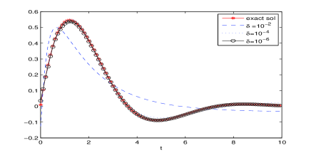
  Figure 5: Example 5: the stability of the approximate solution

  Table 5: Example 5.

  ${\delta}$	$MAE$	$m_{n_{\delta}}$	$Iter.$	CPU time (seconds)	$a_{n_{\delta}}$
  $1.00\times 10^{-2}$	$4.26\times 10^{-2}$	$30$	$3$	$6.300\times 10^{-2}$	$2.00\times 10^{-3}$
  $1.00\times 10^{-4}$	$1.25\times 10^{-2}$	$30$	$3$	$9.38\times 10^{-2}$	$2.00\times 10^{-6}$
  $1.00\times 10^{-6}$	$1.86\times 10^{-3}$	$54$	$4$	$3.13\times 10^{-2}$	$2.00\times 10^{-9}$

  This is an example of the damped sine function. In [2] and [8] the knowledge of the exact data $F(p)$ in the complex plane is required to get the approximate solution. Here we only use the knowledge of the discrete perturbed data $F_{\delta}(p_{j})$, $j=0,1,2,\ldots,m,$ and get a satisfactory result which is comparable with the results given in [2] and [8] when the level noise ${\delta}=10^{-6}$. The reconstruction of the exact solution $f_{5}(t)$ obtained by our method is better than this of the method given in [4]. Moreover, our method yields stable solution with respect to the noise level ${\delta}$ as shown in Figure 5 and Table 5 show. In this example when $\kappa=0.3$ the value of the parameter $m_{n_{\delta}}$ is bounded by $54$ for the noise level ${\delta}=10^{-6}$ (see Table 5).

• Example 6. (see [10])
  

  $$\begin{split}f_{6}(t)&=\left\{\begin{array}[]{ll}t,&\hbox{$0\leq t<1$,}\\ 3/2-t/2,&\hbox{$1\leq t<3$,}\\ 0,&\hbox{elsewhere.}\end{array}\right.\\ F_{6}(p)&=\left\{\begin{array}[]{ll}3/2,&\hbox{$p=0$,}\\ \frac{1-e^{-p}(1+p)}{p^{2}}+\frac{e^{-3p}+e^{2p}(2p-1)}{2p^{2}},&\hbox{$p>0$.}\end{array}\right.\end{split}$$

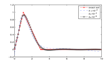
  Figure 6: Example 6: the stability of the approximate solution

  Table 6: Example 6.

  ${\delta}$	$MAE$	$m_{n_{\delta}}$	$Iter.$	CPU time (seconds)	$a_{n_{\delta}}$
  $1.00\times 10^{-2}$	$4.19\times 10^{-2}$	$30$	$2$	$4.700\times 10^{-2}$	$2.00\times 10^{-3}$
  $1.00\times 10^{-4}$	$1.64\times 10^{-2}$	$32$	$3$	$9.38\times 10^{-2}$	$2.00\times 10^{-6}$
  $1.00\times 10^{-6}$	$1.22\times 10^{-2}$	$54$	$4$	$3.13\times 10^{-2}$	$2.00\times 10^{-9}$

  Example 6 represents a class of piecewise continuous functions. ¿From Figure 6 the value of the exact solution at the points where the function is not differentiable can not be well approximated for the given levels of noise by the proposed method. When the noise level ${\delta}=10^{-6}$, our result is comparable with the results given in [10]. Table 6 reports the stability of the proposed method with respect to the noise ${\delta}$. It is shown in Table 6 that the value of the parameter $m$ generated by the proposed adaptive stopping rule is bounded by the constant 54 for the noise level ${\delta}=10^{-6}$ and $\kappa=0.3$ which gives a relatively small computation time.

• Example 7. (see [10])
  

  $$\begin{split}f_{7}(t)&=\left\{\begin{array}[]{ll}-te^{-t}-e^{-t}+1,&\hbox{$0\leq t<1$,}\\ 1-2e^{-1},&\hbox{$1\leq t<10$,}\\ 0,&\hbox{elsewhere,}\end{array}\right.\\ F_{7}(p)&=\left\{\begin{array}[]{ll}3/e-1+9(1-2/e),&\hbox{$p=0$,}\\ e^{-1-p}\frac{e^{1+p}-e(1+p)^{2}+p(3+2p)}{p(p+1)^{2}}+(e-2)e^{-1-p-10p}\frac{e^{10p}-e^{p}}{p},&\hbox{$p>0$.}\end{array}\right.\end{split}$$

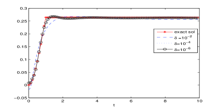
  Figure 7: Example 7: the stability of the approximate solution

  Table 7: Example 7.

  ${\delta}$	$MAE$	$m_{n_{\delta}}$	$Iter.$	CPU time (seconds)	$a_{n_{\delta}}$
  $1.00\times 10^{-2}$	$1.52\times 10^{-2}$	$30$	$2$	$4.600\times 10^{-2}$	$2.00\times 10^{-3}$
  $1.00\times 10^{-4}$	$2.60\times 10^{-3}$	$30$	$3$	$9.38\times 10^{-2}$	$2.00\times 10^{-6}$
  $1.00\times 10^{-6}$	$2.02\times 10^{-3}$	$30$	$4$	$3.13\times 10^{-2}$	$2.00\times 10^{-9}$

  When the noise level ${\delta}=10^{-4}$ and ${\delta}=10^{-6}$, we get numerical results which are comparable with the double precision results given in [10]. Figure 7 and Table 7 show the stability of the proposed method for decreasing ${\delta}$.

• Example 8. (see [3], [4])
  

  $$\begin{split}f_{8}(t)&=\left\{\begin{array}[]{ll}4t^{2}e^{-2t},&\hbox{$0\leq t<10$,}\\ 0,&\hbox{elsewhere.}\end{array}\right.\quad\\ F_{8}(p)&=\frac{8+4e^{-10(2+p)}[-2-20(2+p)-100(2-p)^{2}]}{(2+p)^{3}}.\end{split}$$

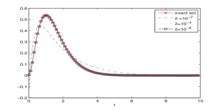
  Figure 8: Example 8: the stability of the approximate solution

  The results of this example are similar to the results of Example 3. The exact solution can be well reconstructed by the approximate solution obtained by our method at the levels noise ${\delta}=10^{-4}$ and ${\delta}=10^{-6}$ (see Figure 8). Table 8 shows that the MAE decreases as the noise level decreases which shows the stability of the proposed method with respect to the noise. In all the levels of noise ${\delta}$ the computation time of the proposed method in obtaining the approximate solution are relatively small. We get better reconstruction results than the results shown in [4]. Our results are comparable with the results given in [3].

  Table 8: Example 8.

  ${\delta}$	$MAE$	$m_{n_{\delta}}$	$Iter.$	CPU time (seconds)	$a_{n_{\delta}}$
  $1.00\times 10^{-2}$	$2.74\times 10^{-2}$	$30$	$2$	$1.100\times 10^{-2}$	$2.00\times 10^{-3}$
  $1.00\times 10^{-4}$	$3.58\times 10^{-3}$	$30$	$3$	$3.13\times 10^{-2}$	$2.00\times 10^{-6}$
  $1.00\times 10^{-6}$	$5.04\times 10^{-4}$	$30$	$4$	$4.69\times 10^{-2}$	$2.00\times 10^{-9}$

• Example 9. (see [18])
  

  $$\begin{split}f_{9}(t)&=\left\{\begin{array}[]{ll}5-t,&\hbox{$0\leq t<5$,}\\ 0,&\hbox{elsewhere,}\end{array}\right.\\ F_{9}(p)&=\left\{\begin{array}[]{ll}25/2,&\hbox{$p=0$,}\\ \frac{e^{-5p}+5p-1}{p^{2}},&\hbox{$p>0$.}\end{array}\right.\end{split}$$

  Figure 9: Example 9: the stability of the approximate solution

  As in Example 6 the error of the approximate solution at the point where the function is not differentiable dominates the error of the approximation. The reconstruction of the exact solution can be seen in Figure 9. The detailed results are presented in Table 9. When the double precision is used, we get comparable results with the results shown in [18].

  Table 9: Example 9.

  ${\delta}$	$MAE$	$m_{n_{\delta}}$	$Iter.$	CPU time (seconds)	$a_{n_{\delta}}$
  $1.00\times 10^{-2}$	$2.07\times 10^{-1}$	$30$	$3$	$6.25\times 10^{-2}$	$2.00\times 10^{-6}$
  $1.00\times 10^{-4}$	$7.14\times 10^{-2}$	$32$	$4$	$3.44\times 10^{-1}$	$2.00\times 10^{-9}$
  $1.00\times 10^{-6}$	$2.56\times 10^{-2}$	$54$	$5$	$3.75\times 10^{-1}$	$2.00\times 10^{-12}$

• Example 10. (see [5])
  

  $$\begin{split}f_{10}(t)&=\left\{\begin{array}[]{ll}t,&\hbox{$0\leq t<10$,}\\ 0,&\hbox{elsewhere,}\end{array}\right.\\ F_{10}(p)&=\left\{\begin{array}[]{ll}50,&\hbox{$p=0$,}\\ \frac{1-e^{-10p}}{p^{2}}-\frac{10e^{-10p}}{p},&\hbox{$p>0$.}\end{array}\right..\end{split}$$

  Figure 10: Example 10: the stability of the approximate solution

  Table 10: Example 10.

  ${\delta}$	$MAE$	$m_{n_{\delta}}$	$Iter.$	CPU time (seconds)	$a_{n_{\delta}}$
  $1.00\times 10^{-2}$	$2.09\times 10^{-1}$	$30$	$3$	$3.13\times 10^{-2}$	$2.00\times 10^{-6}$
  $1.00\times 10^{-4}$	$1.35\times 10^{-2}$	$32$	$4$	$9.38\times 10^{-2}$	$2.00\times 10^{-9}$
  $1.00\times 10^{-6}$	$3.00\times 10^{-3}$	$54$	$4$	$2.66\times 10^{-1}$	$2.00\times 10^{-9}$

  Table 10 shows the stability of the solution obtained by our method with respect to the noise level ${\delta}$. We get an excellent agreement between the exact solution and the approximate solution for all the noise levels ${\delta}$ as shown in Figure 10.

• Example 11. (see [5], [16])
  

  $$\begin{split}f_{11}(t)&=\left\{\begin{array}[]{ll}\sin(t),&\hbox{$0\leq t<10$,}\\ 0,&\hbox{elsewhere,}\end{array}\right.\\ F_{11}(p)&=\frac{1-e^{-10p}(p\sin(10)+\cos(10))}{1+p^{2}}.\end{split}$$

  Figure 11: Example 11: the stability of the approximate solution

  Here the function $f_{11}(t)$ represents the class of periodic functions. It is mentioned in [16] that oscillating function can be found with acceptable accuracy only for relatively small values of $t$. In this example the best approximation is obtained when the noise level ${\delta}=10^{-6}$ which is comparable with the results given in [5] and [16]. The reconstruction of the function $f_{11}(t)$ for various levels of the noise ${\delta}$ are given in Figure 11. The stability of the proposed method with respect to the noise ${\delta}$ is shown in Table 11. In this example the parameter $m_{n_{\delta}}$ is bounded by the constant $54$ when the noise level ${\delta}=10^{-6}$ and $\kappa=0.3$.

  Table 11: Example 11.

  ${\delta}$	$MAE$	$m_{n_{\delta}}$	$Iter.$	CPU time (seconds)	$a_{n_{\delta}}$
  $1.00\times 10^{-2}$	$2.47\times 10^{-1}$	$30$	$3$	$9.38\times 10^{-2}$	$2.00\times 10^{-6}$
  $1.00\times 10^{-4}$	$4.91\times 10^{-2}$	$32$	$4$	$2.50\times 10^{-1}$	$2.00\times 10^{-9}$
  $1.00\times 10^{-6}$	$2.46\times 10^{-2}$	$54$	$5$	$4.38\times 10^{-1}$	$2.00\times 10^{-12}$

• Example 12. (see [3], [5])
  

  $$\begin{split}f_{12}(t)&=\left\{\begin{array}[]{ll}t\cos(t),&\hbox{$0\leq t<10$,}\\ 0,&\hbox{elsewhere,}\end{array}\right.\\ F_{12}(p)&=\frac{(p^{2}-1)-e^{-10p}(-1+p^{2}+10p+10p^{3})\cos(10)}{(1+p^{2})^{2}}\\ &+\frac{e^{-10p}(2p+10+10p^{2})\sin(10)}{(1+p^{2})^{2}}.\end{split}$$

  Figure 12: Example 12: the stability of the approximate solution

  Here we take an increasing function which oscillates as the variable $t$ increases over the interval $[0,10)$. A poor approximation is obtained when the noise level ${\delta}=10^{-2}$. Figure 12 shows that the exact solution can be approximated very well when the noise level ${\delta}=10^{-6}.$ The results of our method are comparable with these of the methods given in [3] and [5]. The stability of our method with respect to the noise level is shown in Table 12.

  Table 12: Example 12.

  ${\delta}$	$MAE$	$m_{n_{\delta}}$	$Iter.$	CPU time (seconds)	$a_{n_{\delta}}$
  $1.00\times 10^{-2}$	$1.37\times 10^{0}$	$96$	$3$	$9.38\times 10^{-2}$	$2.00\times 10^{-6}$
  $1.00\times 10^{-4}$	$5.98\times 10^{-1}$	$100$	$4$	$2.66\times 10^{-1}$	$2.00\times 10^{-9}$
  $1.00\times 10^{-6}$	$2.24\times 10^{-1}$	$300$	$5$	$3.44\times 10^{-1}$	$2.00\times 10^{-12}$

• Example 13.
  

  $$f_{13}(t)=e^{-t},\quad F_{13}(p)=\frac{1}{1+p}.$$

  Here the support of $f_{13}(t)$ is not compact. From the Laplace transform formula one gets

  $$\begin{split}F_{13}(p)&=\int_{0}^{\infty}e^{-t}e^{-pt}dt=\int_{0}^{b}e^{-(1+p)t}dt+\int_{b}^{\infty}e^{-(1+p)t}dt\\ &=\int_{0}^{b}f_{13}(t)e^{-pt}dt+\frac{e^{-(1+p)b}}{1+p}:=I_{1}+I_{2},\end{split}$$

  where ${\delta}(b):=e^{-b}.$ Therefore, $I_{2}$ can be considered as noise of the data $F_{13}(p)$, i.e.,

  $$F_{13}^{\delta}(p):=F_{13}(p)-{\delta}(b),$$ (128)

  where ${\delta}(b):=e^{-b}.$ In this example the following parameters are used: $d=2$, $\kappa=10^{-1}$ for ${\delta}=e^{-5}$ and $\kappa=10^{-5}$ for ${\delta}=10^{-8},$ $10^{-20}$ and $10^{-30}$. Table 13 shows that the error decreases as the parameter $b$ increases. The approximate solution obtained by the proposed method converges to the function $f_{13}(t)$ as $b$ increases (see Figure 13).

  Table 13: Example 13.

  $b$	$MAE$	$m_{\delta}$	Iter	CPU time (seconds)
  $5$	$1.487\times 10^{-2}$	2	4	$3.125\times 10^{-2}$
  $8$	$2.183\times 10^{-4}$	2	4	$3.125\times 10^{-2}$
  $20$	$4.517\times 10^{-9}$	2	4	$3.125\times 10^{-2}$
  $30$	$1.205\times 10^{-13}$	2	4	$3.125\times 10^{-2}$

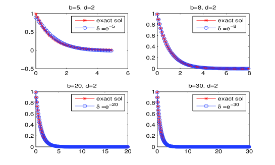
  Figure 13: Example 13: the stability of the approximate solution

4 Conclusion

We have tested the proposed algorithm on the wide class of examples considered in the literature. Using the rule (63) and the stopping rule (87), the number of terms in representation (73), the discrete data $F_{\delta}(p_{j})$, $j=0,1,2,\ldots,m$, and regularization parameter $a_{n_{\delta}}$, which are used in computing the approximation $f_{m}^{\delta}(t)$ (see (73)) of the unknown function $f(t)$, are obtained automatically. Our numerical experiments show that the computation time (CPU time) for approximating the function $f(t)$ is small, namely CPU time $\leq 1$ seconds, and the proposed iterative scheme and the proposed adaptive stopping rule yield stable solution with respect to the noise level ${\delta}$. The proposed method also works for $f$ without compact support as shown in Example 13. Moreover, in the proposed method we only use a simple representation (73) which is based on the kernel of the Laplace transform integral, so it can be easily implemented numerically.