Temperature dependence of the magnetic Casimir-Polder interaction
Abstract
We analyze the magnetic dipole contribution to atom-surface dispersion forces. Unlike its electrical counterpart, it involves small transition frequencies that are comparable to thermal energy scales. A significant temperature dependence is found near surfaces with a nonzero dc conductivity, leading to a strong suppression of the dispersion force at . We use thermal response theory for the surface material and discuss both normal metals and superconductors. The asymptotes of the free energy of interaction and of the entropy are calculated analytically over a large range of distances. Near a superconductor, the onset of dissipation at the phase transition strongly changes the interaction, including a discontinuous entropy. We discuss the similarities with the Casimir interaction between two surfaces and suggest that precision measurements of the atom-surface interaction may shed light upon open questions around the temperature dependence of dispersion forces between lossy media.
pacs:
03.70.+k – theory of quantized fields; 34.35.+a – interactions of atoms with surfaces; 42.50.Pq – cavity quantum electrodynamics; 42.50.Nn – quantum optical phenomena in conducting media.I Introduction
Ever since the work of Lennard-Jones Lennard-Jones has the interaction between atoms and surfaces been of interest in many fields of physics, chemistry and technology. The seminal work by Casimir and Polder Casimir48a demonstrated that the shift in atomic energy levels close to a conductor is a probe for the quantum fluctuations of the electromagnetic field, a key concept of quantum electrodynamics (QED). In this context, a nonzero temperature becomes relevant for several aspects of the atom-surface interaction: thermally excited motion of the surface (phonons) and inelastic scattering of atomic beams Zangwill ; Desjonqueres ; Farias , occupation of excited atomic energy levels, and enhancement of field fluctuations due to thermal photons Barton72 . The latter aspect is usually associated with distances from the surface larger than the thermal wavelength , approximately at room temperature. The free energy of interaction typically shows a change in power law with distance around this point: generally, it is enhanced with respect to zero temperature and becomes proportional to . This is the classical limit where the interaction is mainly entropic in character Balian77 ; Balian78 ; Feinberg01 .
Experimental progress in recent years has achieved the sensitivity required to detect the small energy shifts that occur at distances on the order of , making use of the exquisite control over the motion of atomic beams (beam deflection Sandoghar ; Sukenik , quantum reflection Shimizu ; Druzhinina ) or clouds of ultracold laser-cooled atoms Yuju2000 ; Obrecht07 . The latter can be handled precisely in miniaturized traps implemented near solid state surfaces known as atom chips Folman ; Hansel01 ; Fortagh . These devices use optical or magnetic fields for trapping and can hold atomic clouds at distances down to a few microns. Here, the atom-surface interaction manifests itself typically as a distortion of the trapping potential (loss of atoms through tunneling to the surface or change in the trap oscillation frequency). Therefore, the design of such setups requires exact knowledge of atom-surface interactions and conversely, theory predictions can be tested experimentally with high precision.
A surprising result of the research on atom chips is the importance of magnetic field fluctuations near the surface arising from thermally excited currents in the material of the chip (Johnson noise related to Ohmic dissipation). These fluctuations couple to the spin magnetic moment of the trapped atoms and are known to provoke the loss of atoms from the trap by flipping the sign of the potential Henkel99 ; Zhang05 . These losses are a main obstacle for technical applications and further down-scaling of atom chips. Predictions that superconducting materials reduce the spin-flip induced losses significantly have recently been backed by trap lifetime measurements Skagerstam2006 ; Hohenester2007 ; Dikovsky2009 ; Emmert2009 ; Hufnagel2009 ; Kasch2009 .
In this paper, we address the magnetic dipole contribution to the atom-surface (Casimir-Polder) interaction including nonzero temperature. One would expect this to be a small correction to the electric dipole coupling McLachlan63a ; Wylie85 ; Milonni94 ; Sols82 ; Buhmann07a ; Bezerra08 because of the smallness of the transition matrix elements Bimonte2009a ; Skagerstam09 . Yet, the strong magnetic mode density close to a metallic surface Jackson75 ; Joulain03 ; Henkel05a and experimental evidence for magnetic spin flips call for a reconsideration of the magnetic contribution. In addition, the thermal occupation of photonic modes is quite relevant because magnetic transitions occur at much lower frequencies than electric ones, leading to a stronger temperature dependence. Finally, it is well-known that dispersion forces between dielectric and magnetic materials can be repulsive daSilva01 , as has been shown for the magnetic Casimir-Polder interaction at in Ref.Henkel05a . We were thus led to investigate whether at distances beyond the total atom-surface interaction might be reduced due to the magnetic contribution.
In this work, we calculate the magnetic Casimir-Polder free energy of interaction at different temperatures and consider a few well-known models for the electromagnetic response of the surface. Since Ohmic losses are crucial for the thermal behavior, it is highly interesting to compare both normal metals and superconductors. The latter are described here in the frame of the two-fluid model and Bardeen-Cooper-Schrieffer (BCS) theory Bardeen57 ; Schrieffer99 . We demonstrate that the magnetic atom-surface coupling has very peculiar features unknown from its electrical equivalent. We find that for normal conductors at nonzero temperature, the magnetic dipole contribution to the interaction is reduced, while it is enhanced for superconductors and in certain non-equilibrium situations. This resembles the macroscopic Casimir interaction between two dissipative plates, where the correct calculation of the force at large distances and nonzero temperatures has been the subject of debate Bostrom2000 ; Milton09a ; Klimchitskaya09 .
This article is organized as follows. In Sec. II, we give a brief review of the formalism used to calculate atom-surface interactions. Section III presents the specific forms of the response functions and the experimental setups they describe. We also give expressions for the Green’s tensor in different asymptotic regimes of the distance between the atom and the surface. The magnetic Casimir-Polder free energy and entropy of an atom near metallic or superconducting surfaces at zero temperature is calculated in Sec. IV. Section V covers the effects at nonzero temperature and discusses the dissipative reduction in the interaction and questions connected to the entropy. Non-thermal (out-of-equilibrium) states of the atoms that occur typically in experimental setups are investigated in Section VII. We conclude summarizing and discussing the main results. Further technical details are given in the appendices.
II Atom-surface interaction
Quite a lot of research has been done on the interaction between an atom and a surface Casimir48a ; McLachlan63a ; Wylie85 ; Milonni94 ; Sols82 ; Buhmann07a ; Bezerra08 ; Bimonte2009a ; Skagerstam09 . It can been shown from perturbation theory with respect to the multipolar atom-field coupling McLachlan63a that the free energy of a polarizable particle at nonzero temperature has the following general form (Einstein summation convention)
| (1) |
Here, is the (magnetic or electric) polarizability tensor for the atom in a thermal state of temperature , and is the (corresponding) Green’s tensor in the presence of the surface, defined in Eq.(4) below. In the planar geometry we are interested in, the Green’s tensor depends only on the atom-surface distance and on frequency. It is well known that Eq.(1) has the same form for electric or magnetic dipole couplings Buhmann07a ; Boyer74 ; our notation is adapted to the magnetic case. A simple and general derivation of Eq.(1) can be given following Refs.Henkel2002 ; Novotny08 . The effective interaction potential between a polarizable particle and the (magnetic or electric) field Jackson75 is given by
| (2) |
The expectation value is taken in an equilibrium state of the non-coupled system at temperature and implicitly evaluates symmetrically ordered operator products; is the (magnetic or electric) dipole operator and the corresponding field operator, evaluated at the atom position . The factor arises from a coupling constant integration (excluding a permanently polarized atom). Within first-order perturbation theory, both the dipole moment and the field can be split into fluctuating (fl) and induced (in) parts: the fluctuating part describes the intrinsic equilibrium fluctuation, while the induced part arises in perturbation theory from the dipole coupling Mandel95 . Eq.(2) becomes
| (3) |
Here, we assume the fluctuating parts of the dipole and of the field to be decorrelated at this order. This assumption would break down at higher orders of perturbation theory. Note that while in Eq.(2), the total dipole and field operators (Heisenberg picture) commute at equal times, this is no longer true for their ‘in’ and ‘fl’ constituents in Eq.(3). The induced quantities are given, in frequency space, by the retarded response functions Jackson75
| (4) | |||
where the frequency dependence allows for a temporal delay. The equilibrium fluctuations follow from the fluctuation-dissipation theorem Callen51
| (5) | |||||
| (6) | |||||
Combining Eqs.(3–6), we recover Eq.(1), setting . One uses the fact that the imaginary part of both Green’s tensor and polarizability tensor are odd in (retarded response functions). The field correlations are needed at the same position , and it is easy to remove the divergent free-space contribution (Lamb shift) from , by keeping in the Green’s tensor only the reflected part of the field Wylie85 . In a planar geometry, it follows from symmetry that the result can only depend on the dipole-surface distance . Note that the Green’s tensor can also depend on temperature through the surface reflectivity. In a two-level model for the atom, the thermal polarizability contains a stronger -dependence because of a Fermi-Dirac-like statistics Callen51 , see Eq.(25) below.
Eq.(1) is often expressed in an equivalent form using the analyticity of and in the upper half of the complex frequency plane. Performing a rotation onto the imaginary frequency axis yields the so-called Matsubara expansion Matsubara55
| (7) |
where are the Matsubara frequencies and the prime in the sum indicates that the term must be weighted by a prefactor . Both and are real expressions for .
If the atom is in a well defined state rather than in a thermal mixture, we have the expression of Wylie and Sipe Wylie85
| (8) |
where is the state-specific polarizability McLachlan63 ; Wylie85
| (9) |
Here, are the dipole matrix elements, is the frequency of the virtual transition ( for a transition to a state of lower energy). Finally, the thermal occupation of photon modes
| (10) |
in the second term in Eq.(8) is the Bose-Einstein distribution. At it occurs only for excited states, for which for (see Eqs.(4.3, 4.4) of Ref.Wylie85 ). The real part of the Green’s tensor can be given an interpretation from the radiation reaction of a classical dipole oscillator Wylie85 . Similarly, this term is practically absent for the electric Casimir-Polder interaction of ground-state atoms because of the higher transition frequencies, .
In the following, we call the Matsubara sum (first line) in Eq.(8) the non-resonant contribution, and the second line the resonant one, because it involves the field response at the atomic transition frequency.
III Response functions
The formalism presented in the previous section is quite general and [] could represent either the magnetic or electric polarizability [Green’s tensor], respectively. We now give the specific forms of these quantities in the magnetic case, focusing on a planar surface and specific trapping scenarios.
III.1 Green’s tensors and material response
The Green’s tensor for a planar surface can be calculated analytically. Let the atom be on the positive -axis at a distance from a medium occupying the half-space below the -plane. By symmetry, the magnetic Green’s tensor is diagonal and invariant under rotations in the -plane:
| (11) |
where is the vacuum permeability and , and are the Cartesian dyadic products. We consider here a local isotropic, nonmagnetic bulk medium [], so that the Fresnel formulae give the following reflection coefficients in the TE- and TM-polarization (also known as - and -polarization) Jackson75
| (12) |
where , are the propagation constants in vacuum and in the medium, respectively (roots with )
| (13) |
and is the modulus of the in-plane wavevector. Note that the magnetic Green’s tensor can be obtained from the electric one by swapping the reflection coefficients Henkel99
| (14) |
All information about the optical properties of the surface is encoded in the dielectric function . We will use four different commonly established descriptions, each of which includes Ohmic dissipation in a very characteristic way. As it turns out, the magnetic Casimir-Polder interaction is much more sensitive to dissipation than the electric one (see Sec.V.3). This is due to the fact that the resonance frequencies in the magnetic polarizability are much lower (see Sec.III.3).
The first model is a Drude metal Jackson75
| (15) |
where is the plasma frequency and is a phenomenological dissipation rate. This is the simplest model for a metal with finite conductivity. If is constant (independent of temperature), the conductivity can be attributed to impurity scattering in the medium.
The second model is the dissipationless plasma model : here, one sets in the right-hand side of Eq.(15). This corresponds to a purely imaginary conductivity.
In the context of atom chips, the case of a superconductor is particularly interesting because dissipation is suppressed as the temperature drops below the critical temperature . We adopt here (third model) a description in terms of the two-fluid model, a weighted sum of a dissipationless supercurrent response (plasma model) and a normal conductor response
| (16) | |||||
| (17) |
where the order parameter follows the Gorter–Casimir rule Schrieffer99 . At , the superconductor coincides with the plasma model, as is known from the London theory of superconductivity London35 . The plasma model is thus the simplest description of a superconductor at zero temperature rather than a model for a normal metal. More involved descriptions of superconductors (including BCS theory) also reproduce the plasma behavior at low frequencies ( well below the BCS gap) and temperature close to absolute zero. The full BCS theory of superconductivity can be applied in this context, too, using its optical conductivity Mattis58 ; Zimmermann91 ; Berlinsky93 , as recently discussed in Ref.BCSunpub . We shall see below (Sec.V.2), however, that the two-fluid model and BCS theory give very close results for realistic choices of the physical parameters.
Our fourth model takes a look at the peculiar case of a very clean metal. Here, rather than by impurity scattering, dissipation is dominated by electron-electron or electron-phonon scattering. In these cases, the dissipation rate in the Drude formula (15) follows a characteristic power law
| (18) |
at small temperatures and saturates to a constant value at high temperatures (Bloch-Grüneisen law). It is reasonable to call this system the perfect crystal model. As in a superconductor, dissipation is turned on by temperature, but in a completely different manner. This can be distinguished in the atom-surface interaction potential.
III.2 Distance dependence of the Green’s tensors
For the Drude model, there are three different regimes for the atom-surface distance that are determined by physical length scales of the system (see Ref.Henkel05a for a review): the skin depth in the medium,
| (19) |
where is the plasma wavelength, and the photon wavelength in vacuum,
| (20) |
Note that for frequencies (Hagen-Rubens regime). This is the relevant regime for the relatively low magnetic resonance frequencies. We then have which leads to the following three domains: (i) the sub-skin-depth region, , (ii) the non-retarded region, , and (iii) the retarded region: . In zones (i) and (ii), retardation can be neglected (van-der-Waals zone), while in zone (iii), it leads to a different power law (Casimir-Polder zone) for the atom-surface interaction.
Since the boundaries of the three distance zones depend on frequency, the respective length scales differ by orders magnitude between the magnetic and the electric case. For electric dipole transitions, the Hagen–Rubens regime cannot be applied because the resonant photon wavelength is much smaller. The role of the skin depth is then taken by the plasma wavelength . This implies that the Casimir-Polder zone (iii) for the electric dipole interaction occurs in a range of distances where magnetic retardation is still negligible [zones (i) and (ii)].
In the three regimes, different approximations for the reflection coefficients that appear in the Green’s function (11) can be made. We start with the Drude model where in the sub-skin-depth zone Henkel99 , we have and
| (21) |
At intermediate distances in the non-retarded zone, the wavevector is , hence,
| (22) |
Finally, in the retarded zone we can consider , so that
| (23) |
A similar asymptotic analysis can be performed for the other model dielectric functions. It turns out that Eqs.(21–23) can still be used, provided the assumption holds. This is indeed the case for a typical atomic magnetic dipole moment and a conducting surface.
The asymptotics of the Green’s functions that correspond to these distance regimes are obtained by performing the -integration in Eq.(11) with the above approximations for the reflection coefficients. The results are collected in Table 1. One notes that the -component is larger by a factor compared to the - and -components. The difference between the normal and parallel dipoles can be understood by the method of images Jackson75 . Furthermore, the magnetic response for a normally conducting metal in the sub-skin-depth regime is purely imaginary and scales linearly with the frequency – the reflected magnetic field is generated by induction. Only the superconductor or the plasma model can reproduce a significant low-frequency magnetic response, via the Meißner-Ochsenfeld effect. In contrast, the electric response is strong for all conductors because surface charges screen the electric field efficiently.
The imaginary part of the Green’s functions determines the local mode density (per frequency) for the magnetic or electric fields Joulain03 . These can be compared directly after multiplying by (or ), respectively. As is discussed in Refs.Joulain03 ; Henkel05a , in the sub-skin-depth regime near a metallic surface, the field fluctuations are mainly of magnetic nature. This can be traced back to surface charge screening that efficiently decouples the interior of the metal and the vacuum above. Magnetic fields, however, cross the surface much more easily as surface currents are absent (except for superconductors). This reveals, in the vacuum outside the metal, the thermally excited currents from the bulk.
| Sub - | skin depth | Non-retarded | Retarded | |||
|---|---|---|---|---|---|---|
| Drude | plasma | |||||
III.3 Atomic polarizability
The magnetic and electric polarizabilities are determined by the transition dipole matrix elements and the resonance frequencies. We are interested in the retarded response function, which for an arbitrary atomic state is given by Eq.(9) above.
When the atom is in thermal equilibrium, we have to sum the polarizability over the states with a Boltzmann weight:
| (24) |
where is the partition function. In the limit , we recover the polarizability for a ground state atom. For a two-level system with transition frequency , the previous expression takes a simple form and can be expressed in terms of the ground state polarizability [Eq. (9), where ]:
| (25) |
Let us now compare the electric and magnetic polarizabilities. The magnetic transition moment among states with zero orbital spin scales with where is the Landé factor for the electron spin and the Bohr magneton. Electric dipoles are on the order with the Bohr radius. With the estimate that the resonance frequencies ( and ) determine the relevant range of frequencies, we have approximately
| (26) |
where is the fine-structure constant. The magnetic interaction is thus expected to be a small correction. Conversely, the narrower range of frequencies makes it much more sensitive to the influence of temperature.
We have seen now that the polarizability of an atom takes a positive constant value at low frequency and the induced magnetic dipole is parallel to the magnetic field (paramagnetism). Let us consider for comparison a metallic nanosphere. If its radius is smaller than the penetration depth and the wavelength, the polarizability is given by Jackson75
| (27) |
This quantity vanishes at low frequencies and has a negative real part (diamagnetism). For a qualitative comparison to an atom one can estimate, e.g., the magnetic oscillator strength, defined by the integral over the imaginary part of the polarizability at real frequencies
| (28) | |||||
| (29) |
From the Clausius-Mossotti relation follows the electric counterpart:
| (30) |
We find that the nanoparticle has a dominantly electric response, similar to an atom, but the ratio of the oscillator strengths depends on the material parameters and the radius. From the above expressions, we find that the absolute value of the nanosphere’s magnetic oscillator strength is actually smaller than the one of an atom if the sphere’s radius .
III.4 Optical and magnetic traps
The resonance frequencies relevant for the magnetic Casimir-Polder potential depend on the trapping scheme. We focus here on alkali atoms that are typically used in ultracold gases and distinguish between optical and magnetic traps.
In an optical trap, we may consider the case that the magnetic sublevels are degenerate and subject to the same trapping potential (proportional to the intensity of a far-detuned laser beam). Magnetic dipole transitions can then occur between hyperfine levels whose splitting is on the order of , corresponding to temperatures of (see Appendix B for more details.) In contrast, electric dipole transitions occur in the visible range or . If we average over the magnetic sublevels, we get an isotropic magnetic polarizability. This allows to write , so that in Eq.(1) or (7)
| (31) |
The setup we will consider in most of our examples is an atom in a magnetic trap. In these traps, one uses the interaction of a permanent magnetic dipole with an inhomogeneous, static magnetic field . Let us consider for simplicity a spin manifold: the Zeeman effect then leads to a splitting of the magnetic sublevels by the Larmor frequency, in weak fields. To give an order of magnitude, at . Atoms in those magnetic sublevels where are weak-field seekers, and can be trapped in field minima. The magnetic trap we have in mind is a two-wire trap suspended below the surface of an atom chip. Currents in the two wires, combined with a static field, create a field minimum below the chip surface, with gravity pulling the potential minimum into a position where the magnetic field is nonzero and perpendicular to the surface. Magnetic dipole transitions are then generated by the parallel components , of the dipole moment (see Appendix B). In this anisotropic scenario, the components of the magnetic polarizability tensor are given by and . The relevant components of the Green’s tensor are, therefore,
| (32) |
We should mention that many experiments do not realize a global equilibrium situation, as assumed in Eq.(1). In typical atom chip setups, atoms are laser cooled to temperatures or prepared in a well-defined state, while the surface is generally at a much higher temperature, even when superconducting. For the description of such situations, a more general approach à la Wylie and Sipe [Eqs.(8) and (9)] is more suitable, and we discuss the results in Sec.VII. Before addressing these, we start with thermal equilibrium free energies, however. This may be not an unrealistic assumption in spectroscopic experiments where Casimir-Polder energies are measured with atoms near the window of a vapor cell Failache99 . From the theoretical viewpoint, thermal equilibrium provides an unambiguous definition of the entropy related to the atom-surface interaction. We shall see that this quantity shows remarkable features depending on the way dissipation and conductivity is included in the material response. This closely parallels the issue of the thermal correction to the macroscopic Casimir interaction, a subject of much interest lately.
To summarize, in an optical (isotropic) trap, the equilibrium Casimir-Polder free energy (7) is given by the Matsubara sum
| (33) | |||
while in a magnetic (anisotropic) trap, we have
| (34) |
IV Zero-temperature interaction potential
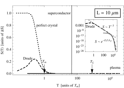
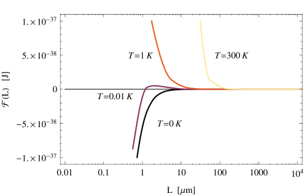
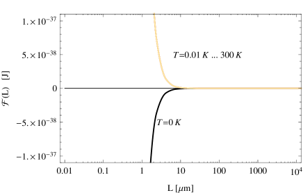
The (free) energy vs. distance has been calculated numerically for an anisotropic magnetic dipole in front of a half-space filled with a normal conductor (Fig.1, top) or described by the plasma model (Fig.1, bottom). The thick black curves give the zero-temperature result (see the caption for parameters). The dashed asymptotes are discussed in this section. All energies are normalized to the power law of the non-retarded Casimir-Polder energy near a perfectly reflecting surface. The scale factor , given in the caption, is slightly smaller than Eq.(38) below. These and the following results have been obtained from the numerical procedure described in Appendix A.
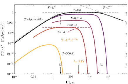
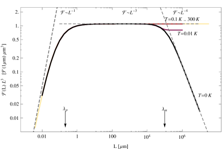
The magnetic Casimir-Polder potential is always repulsive as expected from the interaction between an oscillating magnetic dipole and its image at the conducting surface. The sign is also consistent with the macroscopic Casimir interaction between a conducting and a permeable surface (‘mixed’ Dirichlet-von Neumann boundary conditions), see e.g. Ref.Boyer74 . The curves in Fig.1 make manifest the crossovers between the distance regimes introduced in Sec.III.2 above. The relevant length scales are here the skin-depth , evaluated at the transition frequency (for the normal conductor), the plasma wavelength (for the plasma model), and the transition wavelength . The case of the superconductor is discussed in Sec.V.2 below (Fig.2): within the two-fluid model adopted here, it is identical to the plasma model at zero temperature. The temperature dependence interpolates between the Drude and plasma case, as discussed in Secs.V.1 and V.3.
The zero-temperature (black curves) case for a Drude model has been stated earlier in Ref.Henkel05a ; we give details on the asymptotes. Taking the limit in Eq.(7) recovers the well-known expression
| (35) |
In the sub-skin-depth regime , the distance dependence in the anisotropic case (32) for the Drude model becomes
| (36) |
where is the magnetic transition dipole matrix element, cf. Appendix B. This expression is obtained by using the sub-skin-depth asymptote of the magnetic Green’s tensor (first column of Table 1) under the -integral (35) and cutting the integral off at the border of this regime, , i.e., . The small-distance calculation for the plasma model can be done in a similar way. In both the sub-skin-depth and non-retarded regimes, the Green’s tensor (11) becomes independent of (see Table 1), and the frequency integral depends only on the polarizability. Therefore, no logarithm appears as in the dissipative case, but
| (37) |
In the non-retarded regime (intermediate distances), the interaction energy in the Drude model Henkel05a and in the plasma model behave alike
| (38) |
This is calculated as outlined above for the plasma model. The energy (38) is identical to the interaction of the magnetic dipole with its image, calculated as for a perfectly conducting surface. Indeed, the power law is consistent with the dipole field of a static (image) dipole.
In the retarded region (not discussed in Ref.Henkel05 ), the free energy of the Drude is identical to the one of the plasma model. Retardation effects lead to a change in the power law with respect to shorter distances, identical to the electric Casimir-Polder interaction:
| (39) |
The calculation of this asymptote follows the same lines as in the electric dipole case, see Ref.Wylie85 . Comparing different transition wavelengths (e.g., Zeeman vs hyperfine splitting): the smaller the transition energy, the larger the retarded interaction. The numerical data displayed in Fig. 1 agree very well with all three asymptotes.
Eqs.(38) and (39) illustrate that the magnetic atom-surface interaction is reduced relative to the electric one by the fine-structure constant , as anticipated earlier in Eq.(26). One should bear in mind, of course, that the length scales for the cross-overs into the retarded regime are very different. A crossing of the non-retarded magnetic and the retarded electric potentials would be expected for a distance of order , where it is clear that both energies are already extremely small. In addition, the temperature should be low enough so that the thermal wavelength ( is the first Matsubara frequency)
| (40) |
satisfies . Indeed, we shall see in the following section that a nonzero temperature can significantly reduce the magnetic Casimir-Polder potential.
V Casimir-Polder interaction at nonzero temperature
In this section, we consider the temperature dependence of the Casimir-Polder interaction at global equilibrium, in particular using the temperature-dependent polarizability (25). This provides also a well-defined calculation of the atom-surface entropy, see Sec.VI. Scenarios with atoms prepared in specific magnetic sub-levels are discussed in Sec.VII.
The set of curves in Fig.1 illustrates the strong impact of a nonzero temperature for the Drude (normally conducting) metal: its magnitude is reduced for any distance . In the plasma model (no dissipation), the main effect is the emergence of a different long-distance regime: the thermal regime [Eq.(40)]) where the interaction becomes stronger than at . The latter kind of behavior could have been expected from the thermal occupation of photon modes within the thermal spectrum. The effect in the Drude model is more striking and is explained in Sec.V.3 below. A significant difference with the electric dipole interaction is the fact that it is quite common to have temperatures much larger than the magnetic resonance energies, or . Thermal effects thus start to play a role already in the non-retarded regime, and can be pronounced at all distances.
The usual description of the high-temperature (or Keesom Parsegian ) limit is based on the term in the Matsubara sum (7)
| (41) |
Indeed, the higher terms are proportional to the small factor that appears in the Green’s function . This description is discussed in more detail in the following sections.
V.1 Plasma model
In the plasma model and more generally, for all materials where the reflection coefficient goes to a nonzero static limit, the magnetic Green’s tensor is nonzero as well. The leading order potential in the thermal regime is then given by Eq.(41). For the anisotropic polarizability of Eq.(32), and assuming , the temperature dependence drops out, and we find from a glance at Table 1
| (42) |
(assuming ). This is identical to the zero-temperature result in the non-retarded regime (38), as can also be seen in Fig.1. If the temperature is lower, , but the distance still in the thermal regime, the factor in the static polarizability reduces the interaction slightly ( in Fig.1, bottom).
V.2 Superconductor
The atom-superconductor interaction shows a richer behavior compared to the plasma model, as illustrated in Fig.2.
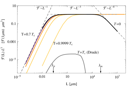
At , it strictly coincides with the plasma model, as it must for the two-fluid description (17) adopted here. The large-distance (thermal) asymptotes are the same as in the plasma model for . The reasoning leading to Eq.(42) can be applied here as well: the response of the superconducting surface to a static magnetic field is characterized by a nonzero value for because of the Meißner-Ochsenfeld effect. Although the superconducting fraction decreases to zero, proportional to the product , the interaction potential Eq.(42) stays constant because it does not depend on this ‘effective plasma frequency’.
This picture also explains the lowering of the sub-skin-depth asymptotes in Fig.2: from Eq.(37), the Casimir-Polder potential is proportional to . This gives scale factors for the cases , in quite good agreement with the numerical data.
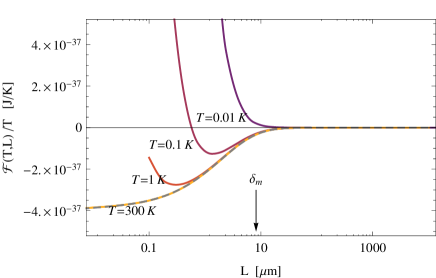
It is worth mentioning that the full BCS theory can give results in close agreement with the simple two-fluid model we use here. In Fig.3, we show the temperature dependence of the Casimir-Polder potential (at fixed distance ) for the two cases. We choose here a damping parameter in the same order of the zero-temperature gap .
The BCS calculations have been performed using a recently developed efficient technique of calculating the optical conductivity at imaginary frequencies BCSunpub and using an approximative form of the gap equation Townsend1962 ; Thouless1960 . Calculations over a larger parameter range, but restricted to , have been reported by Skagerstam et al. Skagerstam09 .
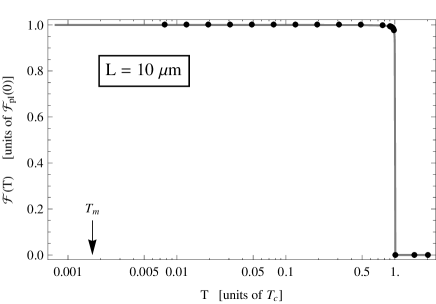
Going back to Fig.2, note that at , the superconductor jumps to a completely different behavior, identical to the Drude metal. This is expected from the two-fluid model (17), but also in Mattis-Bardeen theory where the gap parameter vanishes above , and the optical conductivity coincides with the Drude model, see Refs.Mattis58 ; Zimmermann91 ; Berlinsky93 .
V.3 Thermal decoupling from a normal conductor
As mentioned above, the Drude model and the superconductor around the critical temperature show an unusually strong temperature dependence in the magnetic Casimir–Polder potential. The strong suppression at large distances (Figs.1 and 2) arises from the fact that the Green’s tensor at zero frequency in the normal conducting state. The leading order potential (41) vanishes, and one has to consider the next term in the Matsubara sum 7, so that the exponentially small factor governs the thermal (large distance) regime. We call this the thermal decoupling of the atom from the (normal) metal. This phenomenon is related to low-frequency magnetic fields that penetrate the (non-magnetic) surface. Indeed, the vanishing of could have been expected from the Bohr-van-Leeuwen theorem Leeuwen21 ; Bimonte09 that states that for any classical system, the magnetization response to static fields must vanish. Both conditions apply here: the zeroth term in the Matsubara series involves static fields, and is also known as the classical limit. Indeed, except for the material coupling constants, Eq.(41) no longer involves , while the next Matsubara terms do (via ). The Bohr-van-Leeuwen theorem does not apply to a superconductor whose response is a quantum effect (illustrated, for example, by the macroscopic wave function of Ginzburg-Landau theory), and by extension, not to the plasma model, as recently discussed by Bimonte Bimonte09 .
We now calculate the next order in the Matsubara series to understand the temperature dependence of the Casimir-Polder shift near a metal. For simplicity, we consider again the limiting case which simplifies the polarizability to the Keesom form,
| (43) |
In the thermal regime, , we use the large-distance limit of the Green’s tensor (cf. the retarded regime of Table 1). The Matsubara frequency then yields the mentioned exponential suppression
| (44) |
where is the magnetic resonance wavelength (cf. Fig.1).
At shorter distances, we have to perform the Matsubara summation. In the regime , we consider the non-retarded approximation to the Green’s tensor and make the approximation . The sum over the polarizability can then be done with the approximation (43), and we get
| (45) |
The scaling is in good agreement with Fig.1. The crossover into the sub-skin-depth regime is now temperature-dependent and occurs where the skin depth . This corresponds to a temperature . The involved frequency is characteristic for the diffusive transport of electromagnetic radiation in the metal at wavevectors .
In the sub-skin-depth regime, the leading order approximation to the Matsubara sum involves terms up to a frequency . This leads to an asymptote similar to Eq.(36), but with the ratio in the argument of the logarithm and an additional factor .
VI Atom-surface entropy
It is well-known that at high temperatures where the free energy scales linearly in [Eq.(41)], the dispersion interaction is mainly of entropic origin Parsegian . More precisely, the interaction is proportional to the change in entropy of the system “atom plus field plus metallic surface”, as the atom is brought from infinity to a distance from the surface. We calculate in this section the atom-surface entropy according to
| (46) |
This entropy definition is unambiguous for the global equilibrium setting of the previous Section.
The behavior seen in the previous figures indicates significantly different entropies for the surface models, with a strong dependence on the presence of dissipation (conductivity) at low frequencies. This parallels the discussion of the macroscopic Casimir entropy for the dispersion interaction between two plates, a subject of recent controversies, where the Drude and plasma models give different answers Bezerra04 ; Bostrom04 ; Svetovoy05 ; Sernelius06 ; Intravaia08 ; Klimchitskaya09 . The results that follow indicate that the magnetic Casimir-Polder interaction may provide an alternative scenario to investigate this point.
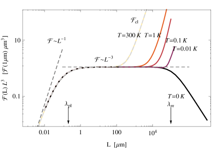
The atom-surface entropy (46) is plotted in Fig.4 for surfaces of different material. In all models, the entropy vanishes at high temperatures because to leading order, the free energy (41) becomes independent of , and higher orders vanish exponentially with . (This feature is specific to the thermal polarizability of a two-level system.) It is remarkable that the vanishing of the entropy happens at temperatures already much smaller than the ‘geometrical scale’ [i.e. with the first Matsubara frequency]. This points towards another characteristic energy scale in the atom-surface system, discussed below.
One notes in Fig.4 very small values for a plasma and a superconductor, two cases where the dc conductivity diverges. The superconductor shows a narrow, pronounced entropy peak at : we interpret this as the participation of the atomic dipole in the phase transition. Indeed, the electromagnetic waves near the surface are slightly shifted in phase due to the interaction with the magnetic dipole moment. The atom-surface interaction can be thought of a sum over all these phase shifts, similar to Feynman’s interpretation of the Lamb shift.
In the Drude model, we observe a broad peak at temperatures where the thermal energy becomes comparable to the photon energy of the magnetic resonance, . Comparable to this scale for our parameters is the diffusive energy , introduced after Eq.(45). We thus attribute the atom-surface entropy to the participation of the atom in the thermally activated diffusive motion of charges and fields below the metal surface (Johnson-Nyquist noise). This motion involves, at the relevant low energies, mainly eddy currents whose contribution to the Casimir entropy (in the plate-plate geometry) has been recently discussed by two of us Intravaia09 . As drops below the diffusive scale , the eddy currents ‘freeze’ to their ground state and the entropy vanishes linearly in .
The dotted curve in Fig.4 corresponds to the ‘perfect crystal’ that has not been discussed so far. It gives rise to a nonzero atom-surface entropy in the limit which is an apparent violation of the Nernst heat theorem (third law of thermodynamics). This has also been discussed for the two-plate interaction Bezerra04 ; Intravaia08 ; Ellingsen09b , but the entropy defect here has a different sign (it is negative for two plates). The sign can be attributed to our atomic polarizability being paramagnetic, while metallic plates show a diamagnetic response. Using the technique exposed in Ref.Intravaia08 , the limit of the atom-surface entropy as can be calculated, with the result for an anisotropic dipole:
| (47) | |||||
The second line applies in the non-retarded limit . This expression is used to normalize the data in Fig.4 and provides good agreement for .
One can argue along the same lines as in Ref.Intravaia09 that the Nernst theorem is actually not applicable for this system, since the perfect crystal cannot reach equilibrium over any finite time in the limit of vanishing dissipation, . The entropy then describes the modification that the atom imposes on the ensemble of field configurations that are ‘frozen’ in the perfectly conducting material.
In the two-plate scenario considered in Refs.Svetovoy05 ; Sernelius06 it has been shown that not only dissipation but also nonlocality of the response has strong implications for the entropy. In particular, the residual entropy vanishes, because at very low temperatures, the anomalous skin effect and Landau damping take the role of a nonzero dissipation rate. Though we have not considered nonlocality in this work explicitly, one can expect the same thing to happen in the magnetic Casimir-Polder interaction.
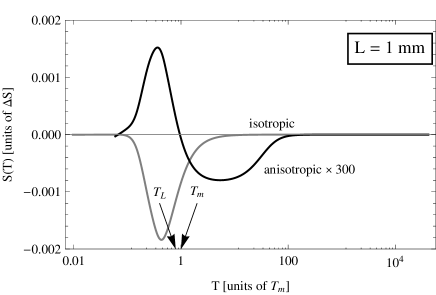
It should be mentioned, that we have also found negative values for the atom-surface entropy, albeit very small, for temperatures between and and in the retarded regime (see Fig.5). The sign depends on the orientation of the dipole and is sensitive to a balance between the TE- and TM-polarized parts of the magnetic Green’s tensor.
VII Non-thermal states
We have argued in the last section, that many realistic setups involve non-equilibrium situations. Atom-chips are a typical example where two independent phenomenological temperatures can be introduced for the atom (or a sample of atoms) and the surface. This temperature gradient is metastable on experimentally relevant time scales because of the weak interaction between the subsystems.
We now analyze the case where the surface is described by a temperature , and the atom prepared in a well-defined state . More complex configurations can be studied starting from this simple case. We first consider two-level atoms and then multilevel atoms, including hyperfine transitions as they occur for the alkali group.
VII.1 Two-state atom
As before, there is a single resonance frequency for the two-level atom. Depending on whether the atom is prepared in the ground-state or the excited state , the sign of the polarizability (9) changes. Referring to the first line of Eq.(8), does no longer depend on temperature. The resonant term of the second line involves the thermal occupation number that we approximate by its classical value . This is sufficiently accurate at room temperature and typical magnetic resonances. In this limit, we obtain a simple expression for the magnetic Casimir-Polder free energy (anisotropic case, argument ‘’ for ground-state atom)
| (48) | |||
The first line is similar to the result in the Drude model because of the missing zeroth Matsubara term. From this expression, we now discuss the differences between the Drude and the plasma model.
For the Drude model, the resonant contribution involving becomes significant in the non-retarded regime. In particular, combined with the non-resonant contribution, it changes the sign of the Casimir-Polder potential already at short distances, resulting in an attractive interaction, as soon as , see Figs.6 and 7.

In contrast, the second line of Eq.(48) nearly vanishes in the plasma model because the magnetic Green’s function is approximately independent of frequency, at least in the non-retarded regime. We thus get a situation where the zeroth Matsubara term is nearly removed from the Casimir-Polder potential. The resonant term still gives the leading order contribution, once the expansion of the occupation number is pushed to the next order, . We then get
| (49) |
where the last expression applies in the non-retarded regime and is identical to the case [Eq.(38)], cf. Fig.8. At larger distances (retarded regime), the difference between the Green’s functions in the second line of Eq.(48) is nonzero and becomes the leading term:
| (50) | |||||
Note that this has a longer range than the power law (49), see Fig.8. This effect is well known from the electric-dipole interaction of excited atoms Hinds91 and consistent with the classical interpretation (frequency shift of an antenna) of the resonant term.
VII.2 Trapped rubidium atom
The atom-surface potential now involves transitions to both higher and lower energy levels. Eq.(8) yields the following form of the free energy
| (51) | ||||
where we assume again that which is valid in many experiments. The sign of the interaction depends on the relative weight of virtual transitions to lower and higher energy levels. From Eq.(9), a virtual level gives a positive contribution to the polarizability and a positive prefactor for the second line in Eq.(51), these terms being negative for levels . We can interpret this sign change from the difference between stimulated emission into the thermal radiation field (for the excited atom) and photon absorption (for the ground state). Generally speaking, these contributions do not cancel each other because the matrix elements are not the same.
Let us consider the example of , prepared in the magnetically trappable hyperfine state of the ground state configuration (Fig.9). This atom has vanishing orbital momentum , nuclear spin , and a single valence electron so that . The splitting between the hyperfine levels (lower) and is , to which the Zeeman splitting in the magnetic trap must be added with the correct Landé factor. We use the same Larmor frequency as before for the two-level atom; because of , we are still in the weak-field regime.

Assuming a quantization axis perpendicular to the surface, see Sec.III.4, we get an anisotropic polarizability. The necessary matrix elements are calculated in Appendix B. Numerical results for the Casimir-Polder interaction according to Eqs.(8) and (9), are shown in Figs. 10 and 11 for the Drude and plasma models, respectively.
Near a normal conducting surface described by the Drude model, the interaction for is attractive at all distances. We associate the sign reversal (compared to the absolute ground state considered so far) to the coupling to the lower-lying Zeeman levels. At high temperatures, the interaction becomes dominated by the resonant contribution that grows linearly with and is repulsive. Again, we find the opposite sign as for the ground-state atom in Fig.6. Thus, the sum of both contributions leads to a maximum of the free energy at a nonzero, -dependent distance.
In the plasma model, the potential crosses over globally (for all distances) from attractive to repulsive. For all practical temperatures, , and the interaction will be repulsive as shown in Fig.11. The results illustrate that the magnetic dipole interaction of an excited atom will be repulsive in all practical realizations.
To summarize, the strong dependence of the thermal correction on dissipation in the surface occurs in both non-equilibrium situations considered here: two-level or multilevel atoms prepared in a given energy state. The magnetic Casimir-Polder potential thus offers an opportunity to distinguish between the two models on the basis of experimental data taken at low surface temperatures and small distances within the possibilities of today’s experiments.
VIII Conclusion and Discussion
We have considered the interaction of a magnetically polarizable particle with a metallic or superconducting surface including the effects of nonzero temperature and out-of-equilibrium situations. Previous work had considered mostly the case of electric polarizability, e.g., Ref.Bezerra08 , or was limited to a static magnetic dipole Bimonte2009a or zero temperature Henkel05a ; Skagerstam09 .
The magnetic atom-surface interaction is repulsive over a large range of parameters and turns out to be highly sensitive to both thermal fluctuations and dissipation. In this respect, it shows similarities with the Casimir interaction between metallic or magneto-dielectric plates.
The results of Ref.Henkel05a suggested that the magnetic interaction might be enhanced by raising the temperature, possibly creating a regime where it dominates over the electric contribution. In fact, thermal enhancement occurs only near a superconductor at distances beyond the thermal wavelength, where the material response is governed by the Meissner effect. In normal conductors, field penetration prevents such a regime – in accordance with the Bohr-Van Leeuwen theorem – and the Casimir-Polder energy is exponentially suppressed in global equilibrium.
This behavior can be understood qualitatively from the competition between attractive and repulsive contributions to the force. Repulsion arises from the fluctuations of the magnetic dipole, coupled to its mirror image. This is similar to the interaction between electric currents (Lenz rule). Field fluctuations, on the other hand, produce attractive forces, due to the paramagnetic character of the atom polarizability. Both contributions differ in their temperature dependence and depend on the state of the atom (thermalized, spin polarized). For example, attractive forces arise between a ground-state atom and a normal conductor, as the temperature scale exceeds the magnetic transition energy. Under realistic conditions, this flips the sign of the interaction in the regime accessible to experiments (Fig.6).
Considering the Casimir-Polder entropy, we found that atoms probe the fluctuations in the material: for instance, at the superconducting phase transition a pronounced peak appears. In most situations, the entropy vanishes at absolute zero in agreement with Nernst’s theorem. The only exception we found was the particular case of a ‘perfect crystal’ [Drude dissipation rate ], already discussed thoroughly in the context of the two-plate Casimir interaction Milton09a ; Klimchitskaya09 . Here, the entropy takes a (positive) nonzero value at zero temperature and can be understood as the participation of the atom in the disorder entropy of currents frozen below the surface Intravaia09 . Indeed, the magnetic dipole moment mimics the current response of a second plate, except for the sign.
If we compare with an electric dipole, the temperature dependence of the Casimir-Polder interaction is relatively weak there. This is due to the larger value of the transition frequency, so that for realistic temperatures there is no difference between the ground-state and the thermalized polarizability. This was assumed in Ref.Bezerra08 , where it was also stated that all good conductors behave very similarly. In fact, the electric dipole coupling is dominated by TM-,polarized modes which cannot penetrate into the bulk due to screening by surface charges.
We have shown here that the Casimir-Polder interaction between a metal and a fluctuating magnetic dipole resembles in many respects the Casimir interaction between two metallic plates. In both scenarios, the thermal dependence is much more pronounced for a normally conducting surface compared to a description without Ohmic losses. The role of dc conductivity in the two-plate scenario is still an open question at nonzero temperature. The atom-surface interaction may thus provide an alternative way to investigate the temperature dependence of the Casimir effect, e.g. in atom chip experiments. The main challenge is the small value of the interaction energy as compared to the electric one. Future measurements of the magnetic Casimir-Polder interaction may involve high precision spectroscopy on the shift in hyperfine or Zeeman levels. In order to separate effects of the magnetic and the electric dipole coupling it will be important to find control parameters that affect exclusively the magnetic contribution. This may include the variation in external fields, isotope shifts, and highly polarizable atomic states like Rydberg atoms.
Acknowledgments
The work of H.H. and C.H. was supported by grants from the German-Israeli Foundation for Scientific Research and Development (GIF). F.I. thanks the Alexander von Humboldt foundation for financial support. The Potsdam group also received support from the European Science Foundation (ESF) within the activity ‘New Trends and Applications of the Casimir Effect’. F.S. acknowledges support from MICINN (Spain), through Grant No. FIS-2007-65723, and the Ramon Areces Foundation. R.P. and S.S. acknowledge partial financial support from Ministero dell’Università e della Ricerca Scientifica and from Comitato Regionale di Ricerche Nucleari e di Struttura della Materia.
Appendix A Numerics
The thermal free energies have then been calculated numerically in the Matsubara-formalism by summing over a thermal spectral free energy density at discrete imaginary frequencies. Now, the infinite sum is replaced by a finite one plus an integral to approximate the remaining infinite partial sum
| (52) |
If the upper summation limit is chosen correctly, the remainder is a slowly varying function and the error is small, according to the Euler-MacLaurin formula. In all systems considered in this work, the exponential in the Green’s function (11) ensures this property.
Numerical calculations require an automatic and fast estimate for the summation limit . In a similar scheme a fixed number of Matsubara terms () has recently been proposed Bostrom04 . It should be pointed out, that since the Matsubara frequencies are linear in , any such scheme with a fixed number of terms breaks down at low temperatures, where the integrand has not sufficiently decayed. A basic criterion for is that the partial sum is sufficiently large, so that the integral is only a small correction
| (53) |
To avoid the evaluation of the integral in Eq.(53) we have used an upper bound
| (54) |
which exploits the exponential decay of introduced by the Green’s tensor. Typically, . In our numerical calculations, we targeted errors and obtained sums over terms. In some cases like BCS theory, the calculation of the optical response is not trivial and the remainder integral was neglected completely. This requires a small enough value of and yields a systematic numeric error .
Appendix B Magnetic transition matrix elements
This section gives the magnetic transition matrix elements used in the calculations of polarizabilities and free energies according to Eqs.(8, 9) or (24).
The simplest approach used is the spin system (two-level atom) with states . The dipole operator is and the quantization axis is ,so that
| (55) | |||||
| (56) | |||||
| (57) |
According to Eq. (25) we need only matrix elements connecting to the ground-state , the only nonvanishing of which yield
| (58) |
Since all polarizabilities (8), (9) or (24) are proportional to the transition frequency, the transitions connecting identical states do not contribute and we obtain the result of Eq. (32).
Let us now calculate the matrix elements for the atom prepared in a hyperfine s-state,
| (59) |
The dipole operator , assuming vanishing orbital momentum and because of the smallness of the nuclear Landé g-factor . We express the states in the uncoupled basis of the spin and nuclear spin momenta with the help of the Clebsch-Gordan coefficients
| (60) |
where the action of the components of the spin operator on a state is known [Eqs.(55-57)]. Hence, we find
| (61) | |||||
| (62) | |||||
| (63) |
References
- (1) J.E. Lennard-Jones, Trans. Faraday Soc. 28, 333 (1932).
- (2) H. B. Casimir and D. Polder, Phys. Rev. 73, 360 (1948).
- (3) A. Zangwill, Physics at Surfaces (Cambridge University Press, Cambridge, England,1988).
- (4) M.-C. Desjonquères, and D. Spanjaard, Concepts in Surface Physics (Springer, New York, 1996).
- (5) D. Farías, and K.-H. Rieder, Rep. Prog. Phys. 61, 1575 (1998).
- (6) G. Barton, Phys. Rev. A 5, 468 (1972).
- (7) R. Balian and B. Duplantier,Ann. Phys. (N. Y.) 104, 300 (1977).
- (8) R. Balian and B. Duplantier, Ann. Phys. (N. Y.) 112, 165 (1978).
- (9) J. Feinberg, A. Mann, and M. Revzen, Ann. Phys. (N. Y.) 288, 103 (2001).
- (10) V. Sandoghdar, C.I. Sukenik, E.A. Hinds, and S. Haroche, Phys. Rev. Lett. 68, 3432 (1992).
- (11) C.I. Sukenik, M.G. Boshier, D. Cho, V. Sandoghdar, and E.A. Hinds, Phys. Rev. Lett. 70, 560 (1993).
- (12) F. Shimizu, Phys. Rev. Lett. 86, 987 (2001).
- (13) V. Druzhinina and M. DeKieviet, Phys. Rev. Lett. 91, 193202 (2003).
- (14) Y.J. Lin, I. Teper, C. Cheng, and V. Vuletic, Phys. Rev. Lett. 92, 050404 (2004).
- (15) J.M. Obrecht, R.J. Wild, M. Antezza, L.P. Pitaevskii, S. Stringari, and E.A. Cornell, Phys. Rev. Lett. 98, 063201 (2007).
- (16) R. Folman, P. Krüger, J. Schmiedmayer, J. Denschlag, and C. Henkel, Adv. At., Mol., Opt. Phys. 48, 263 (2002).
- (17) J. Reichel, Appl. Phys. B: Lasers Opt. 74, 469 (2002)
- (18) J. Fortágh, and C. Zimmermann, Rev. Mod. Phys. 79, 235 (2007).
- (19) C. Henkel, S. Pötting, and M. Wilkens, Appl. Phys. B: Lasers Opt. 69, 379 (1999).
- (20) B. Zhang, C. Henkel, E. Haller, S. Wildermuth, S. Hofferberth, P. Krüger, and J. Schmiedmayer, Eur. Phys. J. D 35, 97 (2005).
- (21) B.S. Skagerstam, U. Hohenester, A. Eiguren, and P.K. Rekdal, Phys. Rev. Lett. 97, 070401 (2006).
- (22) U. Hohenester, A. Eiguren, S. Scheel, and E.A. Hinds, Phys. Rev. A 76, 033618 (2007).
- (23) V. Dikovsky, V. Sokolovsky, B. Zhang, C. Henkel, and R. Folman, Eur. Phys. J. D 51, 247 (2009).
- (24) A. Emmert, A. Lupascu, G. Nogues, M. Brune, J. Raimond, and S. Haroche, Eur. Phys. J. D 51, 173 (2009).
- (25) C. Hufnagel, T. Mukai, and F. Shimizu, Phys. Rev. A 79, 053641 (2009).
- (26) B. Kasch, H. Hattermann, D. Cano, T.E. Judd, S. Scheel, C. Zimmermann, R. Kleiner, D. Kölle, and J. Fortágh, e-print arXiv:0906.1369.
- (27) A. McLachlan, Proc. R. Soc. London, Ser. A 271, 387 (1963).
- (28) J.M. Wylie and J.E. Sipe, Phys. Rev. A 30, 1185 (1984); Phys. Rev. A 32, 2030 (1985).
- (29) P.W. Milonni, The Quantum Vacuum (Academic Press, Boston, 1994).
- (30) F. Sols and F. Flores, Solid State Commun. 42, (1982), 687-690.
- (31) S.Y. Buhmann and D.-G. Welsch, Prog. Quantum Electron. 31, 51 (2007).
- (32) V.B. Bezerra, G.L. Klimchitskaya, V.M. Mostepanenko, and C. Romero, Phys. Rev. A 78, 042901 (2008).
- (33) G. Bimonte, G.L. Klimchitskaya, and V.M. Mostepanenko, Phys. Rev. A 79, 042906 (2009).
- (34) B.S. Skagerstam, P.K. Rekdal, and A.H. Vaskinn, Phys. Rev. A 80, 022902 (2009).
- (35) J.D. Jackson, Classical Electrodynamics (Wiley, New York, 1975).
- (36) K. Joulain, R. Carminati, J.-P. Mulet, and J.-J. Greffet, Phys. Rev. B 68, 245405 (2003).
- (37) C. Henkel, B. Power, and F. Sols, J. Phys.: Conf. Ser. 19, 34 (2005).
- (38) J.C. da Silva, A.M. Neto, H.Q. Plácido, M. Revzen, and A.E. Santana, Physica A 229, 411 (2001).
- (39) J. Bardeen, L.N. Cooper, and J.R. Schrieffer, Phys. Rev. 108, 1175 (1957).
- (40) J.R. Schrieffer, Theory of Superconductivity (Perseus Books, Reading, MA, 1999).
- (41) M. Boström and B.E. Sernelius, Phys. Rev. Lett. 84, 4757-4760 (2000).
- (42) K.A. Milton, J. Phys.: Conf. Ser. 161, 012001 (2009).
- (43) G.L. Klimchitskaya, U. Mohideen, and V.M. Mostepanenko, e-print arXiv:0902.4022, Rev. Mod. Phys. (to be published).
- (44) T.H. Boyer, Phys. Rev. A 9, 2078 (1974).
- (45) C. Henkel, K. Joulain, J.-P. Mulet, and J.-J. Greffet, J. Opt. A 4, S109 (2002).
- (46) L. Novotny and C. Henkel, Opt. Lett. 33, 1029 (2008).
- (47) L. Mandel and E. Wolf, Optical Coherence and Quantum Optics (Cambridge University Press, New York, 1995).
- (48) H.B. Callen and T.A. Welton, Phys. Rev. B 83, 34 (1951).
- (49) T. Matsubara, Prog. Theor. Phys. 14, 351 (1955).
- (50) A. McLachlan, Proc. R. Soc. London, Ser. A 274, 80 (1963).
- (51) F. London and H. London, Proc. R. Soc. London, Ser. A 149, 71 (1935).
- (52) D.C. Mattis and J. Bardeen, Phys. Rev. 111, 412 (1958).
- (53) W. Zimmermann, E. Brandt, M. Bauer, E. Seider, and L. Genzel, Physica C 183, 99 (1991).
- (54) A.J. Berlinsky, C. Kallin, G. Rose, and A.-C. Shi, Phys. Rev. B 48, 4074 (1993).
- (55) G. Bimonte, H. Haakh, C. Henkel, and F. Intravaia, e-print arXiv:0907.3775.
- (56) H. Failache, S. Saltiel, M. Fichet, D. Bloch, and M. Ducloy, Phys. Rev. Lett. 83, 5467 (1999).
- (57) C. Henkel and K. Joulain, EPL 72, 929 (2005).
- (58) V.A. Parsegian, Van der Waals Forces – A Handbook for Biologists, Chemists, Engineers, and Physicists (Cambridge University Press, Cambridge, England, 2006).
- (59) P. Townsend and J. Sutton, Phys. Rev. 128, 591 (1960).
- (60) D.J. Thouless, Phys. Rev. 117, 1256 (1962).
- (61) H.-J. Van Leeuwen, J. Phys. Radium 2, 361 (1921).
- (62) G. Bimonte, Phys. Rev. A 79, 042107 (2009).
- (63) V.B. Bezerra, G.L. Klimchitskaya, V.M. Mostepanenko, and C. Romero, Phys. Rev. A 69, 022119 (2004).
- (64) M. Boström and B. Sernelius, Physica A 339, 53 (2004).
- (65) V.B. Svetovoy and R. Esquivel, Phys. Rev. E 72, 036113 (2005).
- (66) B. Sernelius, J. Phys. A 39, 6741 (2006).
- (67) F. Intravaia and C. Henkel, J. Phys. A 41, 164018 (2008).
- (68) F. Intravaia and C. Henkel, Phys. Rev. Lett. 103, 130405 (2009).
- (69) S.Å. Ellingsen, I. Brevik, J.S. Høye, and K.A. Milton, J. Phys. Conf. Ser. 161, 012010 (2009).
- (70) E.A. Hinds and V. Sandoghdar, Phys. Rev. A 43, 398 (1991).