UMD-PP-09-053
UQAM-PHE-0901
Patterns in the Fermion Mixing Matrix,
a bottom-up approach
Abstract
We first obtain the most general and compact parametrization of the unitary transformation diagonalizing any hermitian matrix , as a function of its elements and eigenvalues. We then study a special class of fermion mass matrices, defined by the requirement that all of the diagonalizing unitary matrices (in the up, down, charged lepton and neutrino sectors) contain at least one mixing angle much smaller than the other two. Our new parametrization allows us to quickly extract information on the patterns and predictions emerging from this scheme. In particular we find that the phase difference between two elements of the two mass matrices (of the sector in question) controls the generic size of one of the observable fermion mixing angles: i.e. just fixing that particular phase difference will “predict” the generic value of one of the mixing angles, irrespective of the value of anything else.
I Introduction
In the absence of flavor symmetries, the Yukawa couplings between the Standard Model (SM) fermions and the Higgs field are in general complex arbitrary matrices which, after Electroweak Symmetry Breaking (EWSB), become the mass matrices of the quarks and charged leptons. In the case of neutrinos, the mass matrix will be in general complex symmetric. All these matrices contain more parameters than physical observables and an explicit computation of these observables (fermion masses and mixings) in terms of the original matrix elements can be quite cumbersome in general. Indeed this would require us to solve a eigenvalue problem for each fermion matrix, and then compose the unitary transformations (formed with the calculated eigenvectors) of the Up and Down quark sectors and then also of the charged lepton and neutrino sectors 555Assuming three families of neutrinos, although additional neutrino flavors are possible (sterile neutrinos).. We observe however that it may be useful to address the question not as an eigenvalue problem, but as an eigenvector problem, treating the eigenvalues as input parameters and not as output. The first reason for this is that except for the neutrino sector, all the mass eigenvalues are quite well known. But the main point we make is that by keeping explicitly the mass eigenvalues as input parameters, the eigenvector solutions of each mass matrix become surprisingly simple and can be written as compact functions of both the mass matrix elements and the eigenvalues (the fermion masses). Such a parametrization of the mixing matrices, directly in terms of the original mass parameters and the fermion masses might prove to be useful in the studies aiming to explain the observed flavor structure of the SM by way of symmetries or textures or patterns Fritzsch1 ; Brokensymmetry ; RRR ; Textures at the level of the fermion mass matrices.
It is true, though, that to proceed we need to work with hermitian matrices, but it is always possible to render the quark mass matrices hermitian in the Standard Model without loss of generality Frampton ; BrancoMota . The procedure to obtain hermitian matrices is quite standard, and it involves either working with the hermitian matrix , where is the original fermion mass matrix, or using its polar decomposition, i.e. solving , where is a unitary matrix converting the general complex matrix into a positive semi-definite hermitian matrix (if is invertible, with distinct non-vanishing eigenvalues, then is positive definite and therefore is unique).
We will first present our parametrization (in fact 9 different types) for the unitary matrix which diagonalizes a general hermitian matrix in the most compact way possible. Then, to start taking advantage of it, we then propose a simple and mildly constraining ansatz for the flavor structure of the SM fermion sector. It assumes that the unitary transformations diagonalizing and can each be decomposed as only two rotations, instead of three. The idea is to assume that the third rotation angle is zero (or much smaller than the other two) and therefore one of the entries of each transformation matrix and will be zero or close to zero. We call this setup the two-angle ansatz and we will concentrate in only one of the many possible cases. Our parametrization allows us to quickly obtain very simple dependences of the fermion mixing matrices and Cabibbo in terms of the masses and the original mass matrix elements. We can thus study easily the interesting properties of this type of ansatz as well as the consequences it has in the original mass matrices, in both the quark and the lepton sectors. A particularly interesting observation is that the specific value of some elements of and has no effect (or very mild effect) on the observed values of masses and mixings.
II Mixing matrix parametrization
As explained before, we are going to concentrate on hermitian matrices with the assumption that the fermion mass matrices are either hermitian or that one can construct a hermitian matrix out of them. All the results presented in this work are valid for general hermitian matrices, but for simplicity we will only consider the case of positive definite hermitian matrices. Let be one such matrix:
| (1) |
with eigenvalues and . A compact parametrization of the unitary matrix which diagonalizes it, is 666There are 9 different ways of parametrizing it, depending on the choice of which diagonal mass parameter ( or ) is explicitly absent in each vector column (see Appendix A for details). In the parametrization shown here, the rotation matrix has the correct limit when the off-diagonal entries in the original mass matrices are set to zero, avoiding (apparent) divergences in this limit.
| (2) |
After some algebra the normalization parameters are found to have the simple form
| (3) | |||||
| (4) | |||||
| (5) |
The surprisingly simple and compact form of this parametrization might make it suitable to treat flavor models keeping always an explicit dependence on all the matrix elements of the hermitian mass matrices. Of course, if the three eigenvalues , and are fixed, there must be three constraint equations on the elements of the matrix . These equations are found from the three invariants , and :
| (6) | |||||
| (7) | |||||
| (8) |
By choosing as an independent variable, it is possible to rewrite these constraint relations on the rest of variables as777The same type of relations can be written when choosing or as the independent variable.
| (9) | |||||
| (10) | |||||
| (11) |
The interesting thing of this notation is that the constraint formulae on and actually become algebraic solutions for both and when the term vanishes identically. In particular, this is the case when one deals with mass matrices with texture zeroes in the off-diagonal elements.
III Flavor in the two-angle ansatz
Equipped with an exact and simple parametrization of the fermion mixing matrix in both Up and Down sectors (or charged lepton and neutrino sectors), we look for economical patterns among the mixing matrices by following a bottom-up approach in the hope that it might be complementary to more top-down approaches such as imposing flavor symmetries or texture zeroes mass matrices (see Fritzsch1 ; Brokensymmetry ; RRR ; Textures as well as the probably incomplete surveys of Flavor ; mutau ). One avenue is to find a similar ansatz for the flavor structure of the mixing matrices in both quark and leptonic sectors. Such possibility exists in the sense that in both sectors, the mixing elements and are known to be small. This feature is very interesting and it is known to lead to a simple parametrization of the mixing matrix. Note that in the limit we have two additional conditions, since is a complex number. This means that in this limit, the mixing matrix will have only two independent parameters instead of four. We can choose these four independent parameters to be , , and CherifModulii . In the limit of , we have the extra constraint . This means that the whole mixing matrix is described by and . Note also that in this limit, there is no violation à la Dirac in both quark and leptonic sectors.
In what follows, the subscript stands for the values of the mixing matrix elements in the limit . Since is known to be very small, we believe that the zeroes values of the mixing matrix elements are not far from their measured values. For the quarks, we have:
| (12) |
Note that this zero-order can be decomposed as a product of two rotations, namely one is purely the Cabbibo angle and the other one is purely made out of beauty namely :
| (13) |
with
| (14) |
In the leptonic sector we have:
| (15) |
which can be decomposed also as a product of two rotations, namely one is purely solar and the other one is purely atmospheric:
| (16) |
with,
| (17) |
The diagonal phase matrix which contains the Majorana phases is defined as:
| (18) |
This structure for the physical fermion mixing matrices, decomposed mainly into just two rotations is quite suggestive and we will use this observation as the starting point of our analysis. In this context we ask ourselves how many economical possibilities one has to restore minimally and fully the mixing elements and violation. We start with the structure
| (19) |
and then to be as general as possible while still keeping the original motivation we consider all mixing patterns emerging from the original structure, but with only one zero in each mixing matrix. Now, we establish all the corrected mixing patterns for both Up and Down quark sectors:
| (20) |
| (21) |
where stands for a non-zero value and for a corrected originally zero mixing matrix element.
These mixing matrices with one texture zero in them can be decomposed
themselves into only two rotations instead of three. We call this the
two-angle ansatz, in which both the Up and Down quark sectors are
diagonalized by unitary transformations containing just two angles
(i.e. having one vanishing element).
There are obviously many possibilities for this ansatz but in particular
there are 16 cases such that one can recover in a specific limit the
case . In this work we are going to focus only on one
specific example of this type of ansatz, although a full case by case
study is underway.
We feel that the main features of this ansatz do reveal
themselves in the example studied here, and we prefer to continue elsewhere
a more systematic exploration.
Notation
Before we proceed further, we will set up
our notation for all the matrices in both up and down quark sectors as
well as charged lepton and neutrino sectors.
We will define the Hermitian matrices , , and defined by:
| (22) |
with eigenvalues and and
| (23) |
with eigenvalues and .
In the text, we will also need to refer to the phases of the off-diagonal terms, denoted as
| (24) | |||
| (25) |
and similarly for the leptons. The matrices diagonalizing these mass matrices will be denoted respectively as , , and .
III.1 THE CASE (13-13):
We will now consider the mass matrices from Eqs. (22) and (23) with the extra constraints of and in the quark sector and and in the lepton sector.888 In the quark sector, this limit was shown to lead to acceptable patterns in the limit and BrancoRebelo and similar limits were considered in the lepton sector in Antusch
III.1.1 The quark sector
For example in the down quark sector imposing corresponds to the requirement . After a short computation, we obtain simpler relations among the elements of the mass matrix:
| (26) |
These relations will simplify significantly the general form of the Down quark mixing matrix as well as the up quark mixing matrix (see Eq. (2) and Appendix B for details).
It is then straightforward to show that the quark mixing matrix takes the form
| (27) |
where and are unphysical diagonal phase matrices given below and
| (28) |
The complex rotation parameters , , and are given by
| (29) | |||||
| (30) | |||||
| (31) | |||||
| (32) |
Note that and that . The CP phase and the two unphysical phase matrices and are given respectively by , and , with .
The previous form of the mixing matrix implies the following exact relations for the quark sector
| (33) |
and
| (34) |
which really correspond to two independent constraints (i.e. the third and fourth relations can be obtained using the first two along with the unitary constraints).
As can be seen only two original mass matrix elements (from ) and (from ) appear explicitly in these last four relations showing the first effect of the ansatz, i.e. linking each of the previous ratios to a different quark mass matrix, and in particular to the first diagonal elements of each mass matrix. Once we fix these two elements to fit the experimental value of the ratios given in Eqs. (33) and (34), we will still have 6 free parameters (including 4 phases) to fit the rest of the data (i.e we need to fit two more scalar observables from experiment, which for example can be taken to be the absolute value of and the value of the CP phase of the fermion mixing matrix). We can choose to use and the phases of and as the free parameters. It is also useful to define the phase combinations:
| (35) | |||||
| (36) | |||||
| (37) |
which have the constraint
| (38) |
due to the ansatz imposition.
Of course, we have more than enough free parameters to fit the two remaining observables, but as we will shortly see, of the 4 free phases, only two phase differences can be relevant, and the 2 real parameters and turn out to be statistically irrelevant if the two phases are properly chosen. In other words, in most of the parameter space of the six free parameters needed to produce the two remaining physical observables, 4 directions are more or less irrelevant, with two phase differences being the two parameters required to obtain a good experimental fit. This situation is somewhat surprising because the amount of “useful” free parameters is less than the total number of free parameters. Let’s see how this is played out.
Eq. (33) shows that and are required in order to obtain a good fit with experimental data PDG . This has interesting implications for since it means that and after using the trace identity of and . We can therefore write
| (39) |
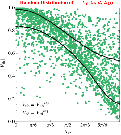
It turns out that when the phase is small (modulo ), statistically we find that for any randomly chosen value of and . In fact, the generic value of is very much correlated with the value of , with little dependence on the values of the other two variables, at least for small enough . This is shown in figure 1, where we plot the distribution of with respect to for randomly chosen values of and . It is apparent that there is a clear correlation between the value of the phase and the value of . The two black curves correspond to the and quantiles of the distribution of for a given value of (i.e. of the randomly generated points lie between the two curves, with above them and below).
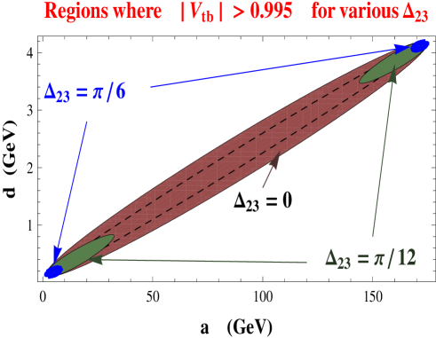
All this shows that the generic value of in this ansatz is actually governed by the specific value of the phase , with very mild dependence on the other 2 parameters and . It is not clear though, that demanding will be enough to fit the observed data in the quark sector since , i.e it is quite close to 1. The random scan of Figure 1 does not show the distribution of for , but once we fix we just have two free parameters, and . In Figure 2 we show the complete allowed phase space for and , which are subject to the experimental constraints and . The different shaded regions are the points where , for three different values of the phase difference . When this last one is zero, the region is quite large, and it decreases very fast as the phase is increased. Because the area of parameter space can be quite large we may still say that the value of consistent with experimental data could be considered “generic” as long as the phase difference is vanishingly small.
Finally, one can also compute quite easily the Jarlskog invariant Jarlskogbook in this context. From Eq. (28), and using for example the definition , it is easy to see that it will have the form:
| (40) |
where , and were given in Eqs. (29), (30), (31) and (32), and where with .
Before analyzing in more detail the dependence on the original mass matrix elements, it is interesting to relate the phase not just to the Jarlskog invariant but also to the angles of the unitarity triangle , and . These angles are defined as:
| (41) | |||||
| (42) | |||||
| (43) |
and the relation between them and the Jarlskog J is:
| (44) |
In the case of our ansatz, we can rewrite our J as
| (45) |
For example, from the first identities of Eq. (44) and (45) one sees that we must have
| (46) |
Since , it follows from the above equation that . The experimental constraints on are such that PDG , which basically means that the phase is constrainted to be .
A more revealing way to see what this means for the original elements of the mass matrices, we can actually rewrite the Jarlskog in a more explicit way as
| (47) | |||||
| (48) |
where the approximation of the second line comes from assuming that and .
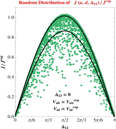
We showed earlier that the imposition of gives a nice statistical reason for the large value of . With that extra condition, one actually has , which then means that due to experimental bounds. The experimental best fit value of the Jarlskog invariant is PDG ; in the right panel of Figure 1 we present a scan of values of the function of shown in Eq. (48), for random values of , and (assuming ). It is apparent that the observed value of can be obtained quite generically when , in a quite insensitive way to the specific values of and .
It is quite suggestive that some specific phase differences between the elements and , and between the elements and and between the elements and , given by:
| (49) | |||
| (50) | |||
| (51) |
do lead to good generic values of both and . We are left with four parameters and two combinations of phases independent of and , all from the original mass matrices, which do not seem to play any important role in obtaining a good overall fit in the quark sector.
Before we finish this subsection on the quark sector, we would like to point out that since and can take almost any value (inside their allowed range), one might actually get very close to a symmetric limit, namely a family symmetry, relating second and third families (see mutau for implementations mostly in the lepton sector).
Forgetting for a moment our ansatz but assuming the limit for both up and down quark mass matrices, one is then guaranteed to have vanishing elements and (i.e. we recover our ansatz). Moreover some of the elements of the mass matrix are subject to the constraints
| (52) | |||||
| (53) | |||||
| (54) |
From these equations, we must have and using Eq. (29) it is easy to see that exactly, which means also that . Since the fitted values of , , and are at most and much smaller than , then it seems plausible that a small deviation from this symmetric limit can easily restore the experimental values of these ’s.
To obtain a correct experimental fit, one would also have to require the phases of and to be separated by (as remarked earlier), and moreover the values of and will have to be chosen so as to obtain the correct ratios and (see Eq. (33)).
Although we imposed a flavor ansatz mainly for empirical reasons and simplicity, it is interesting that the patterns emerging from it do actually lead to a possible type of symmetry. Of course we just considered one of the possible cases of our scheme, and others cases might lead to different patterns or reveal some other feature and for this a more systematic study is required, some of it being already underway.
III.1.2 The lepton sector
In the lepton sector, the mixing matrix takes the same form as for the quarks in the ansatz, i.e.
| (55) |
where is an unphysical diagonal phase matrix given below and
| (56) |
where is the Majorana phase matrix given below and the complex rotation parameters and are given by
| (57) | |||||
| (58) | |||||
| (59) | |||||
| (60) |
Note that and that . The CP phase and the Majorana phase matrix , as well as the unphysical phase matrix are given respectively by , and , where .
Again, the previous form of the mixing matrix implies the relations:
| (61) |
and
| (62) |
with again only two parameters from the original mass matrices separately controlling each ratio.
But, the lepton case is different, obviously, because the lepton mixing matrix contains two large angles and also because the neutrino mass structure is unknown and might not be as hierarchical as in the quark sector (see for example neutrinoexp for the latest global fits coming from neutrino oscillation experiments). In the (13-13) ansatz we see that we must still enforce the charged lepton mass matrix to have a very small first diagonal element, i.e in order to obtain a small value for the ratio . This will imply that (from the trace identity of ) which will simplify the functional form of of Eq. (57). Before doing so, we need to look also into the required value of to obtain a correct fit for in the approximate tri-bimaximal scheme HarrisonPerkinsScott . This leads to , and we can now use this relation to obtain the simplified form of :
| (63) |
where is fixed by the measured atmospheric neutrino mass difference999Although we have been writing and for the neutrino eigenvalues, these could in fact correspond to the squared physical masses if we consider the neutrino mass matrix squared as our starting point. In this case, ..
We now have 7 free parameters (including 4 phases), since one of the neutrino masses is unknown, and we choose it to be .
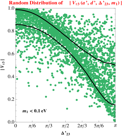
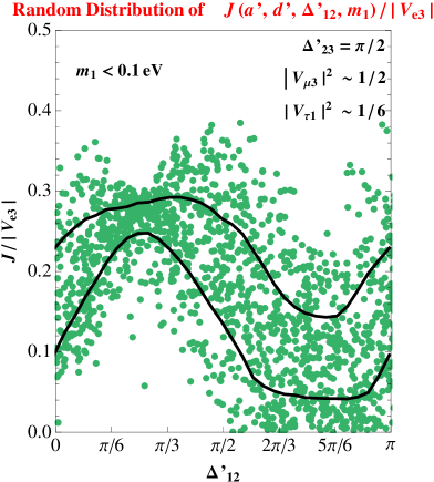
As seen in Figure 3, when eV, the correlation between the phase and the value of is basically the same as it was in the quark sector, and this is basically due to the fact that this feature happens for masses which are hierarchical (and in fact, for larger values of the correlation between the phase and the value of starts to wash out). It is quite suggestive, that if eV and , then we obtain a generic size of , as shown in Figure 3. Because is small, and we will also have . These two values of and are consistent with the tri-bimaximal scheme where and so we find that in the lepton case the preferred value of the phase combination is , which statistically predicts a large value for both the mixing angles and . It is also interesting to note that the charged fermion mass matrix must have the same structure as the up and down quark mass matrices, namely that the first diagonal element is of the order of the lightest eigenvalue.
Since the mixing element is not small, we also conclude that the neutrino mass structure must be different from the other three matrices. This could be due to the fact that the eigenvalues are not as hierarchical as for the charged fermions. As in the quark case, it is interesting to note that further imposing some flavor symmetry might simplify the relations obtained in this ansatz. In particular one could ask what is the effect of imposing the family symmetry (see for example mutau ) only in the neutrino sector. In our case this is a natural question to ask since this symmetry imposes automatically the element to be zero, which is the defining condition of our ansatz. But it also imposes the following constraints on the mass matrix elements
| (64) | |||||
| (65) | |||||
| (66) |
This will have interesting consequences on the lepton mixing matrix because in this case we will have
| (67) |
where we have assumed that . Now one can see that when , independent of anything else, we will have , as well as . Thus the symmetry, along with the requirement of the phase of to be , forces the appearance of large mixing angle in the matrix, and we remind the reader that we are not considering a diagonal charged lepton mass matrix, although all our matrices are taken in the ansatz. The form of the matrix under these assumptions is
| (68) |
where as before, and and where is the Dirac CP phase given by and the Majorana phase matrix is given by
| (69) |
The phase is given by .
Finally, in the more general case where one does not consider symmetry in the neutrino sector, the leptonic Jarlskog invariant is computed to be:
| (70) | |||||
| (71) |
For the preferred value of , such that statistically it is more favorable to obtain a mixing angle close to , we obtain
| (72) |
This suggests that now, the value will maximize the possible value of (normalized to ), and this is confirmed in the random scan shown in Figure 3.
IV Discussion and outlook
In this work, we started by obtaining the simplest parametrization for the diagonalization of a hermitian matrix, as a function of both its matrix elements and its eigenvalues. Since the masses of fermions in the SM are well known, the problem to attack is not an eigenvalue problem, but an eigenvector problem. In other words, we are able to obtain the eigenvectors of a hermitian matrix in an algebraically compact form because we treated the eigenvalues as known parameters, instead of unknown. With this parametrization in hand, we wanted then to show how it could simplify and make quite transparent the analysis and study of some flavor schemes. To this end we defined a new flavor scheme which imposes some (arguably obscure) constraints on the flavor structure in the fermion sector. The constraint imposed is the requirement of the vanishing of one of the mixing angles of the diagonalization matrix of each hermitian fermion mass matrix of the SM. We called this the “two-angle” ansatz (i.e. out of three angles to diagonalize a hermitian matrix, we consider the family of hermitian matrices diagonalized by only two angles), and it is bottom-up motivated, i.e. it is inspired on the observed structure of both and matrices. Nevertheless we also observe that in flavor models where one requires a full symmetry between two of the three families, like the symmetry models, one of the consequences is precisely the vanishing of one of the mixing angles.101010In the case of a complex symmetric neutrino mass matrix, the authors of Lavoura studied the symmetry conditions required for the vanishing of one of the mixing angles of the rotation matrix But we mainly decided to keep the bottom-up approach motivation and study the patterns emerging from our “two-angle” ansatz and focused on just one possible implementation, the case, in which the entries of all the diagonalizing matrices happen to vanish. Using our parametrization, one can actually write both and in terms of the original matrix elements and eigenvalues. In particular we found a peculiar dependence of one of the mixing angles with the model parameters. We observed that by fixing the phase difference between two parameters of the up and down mass matrices (or the neutrino and charged lepton mass matrices), the mixing angle (or ) can be “predicted” in a statistical sense, i.e. if one makes a random scan allowing the remaining free parameters to take any possible value, including the eigenvalues, one obtains a narrow distribution for the value of (or ), and the central value is a monotonic function of the phase difference . This can be seen by rewriting the general formula for in the ansatz (see Eq. (29)) as
| (73) |
where , , and , and and are diagonal elements of the up and down mass matrices respectively. If the mass eigenvalues are unconstrained, the only constraints on the parameters required for a random scan are
| (74) |
since the diagonal elements of a hermitian matrix must be bounded by its largest and lowest eigenvalues. The result of a scan over all these parameters (including the eigenvalues) but for fixed is a highly peaked distribution centered at some value. This means that the generic value of is controlled almost exclusively by . Of course one may think that after fixing the masses to the experimental values, as well as the other mixing angles, maybe we might loose this statistical prediction. This is not the case as was shown in Figure 1, where the scan is performed now with only two free parameters, the rest having been fixed by other experimental observables. There is still a clear correlation between the value of the phase difference and the value of the angle .
The imposition of this specific two-angle ansatz (the () case) on the fermion mass matrices amounts to 2 constraints per mass matrix, and therefore 4 constraints in the quark sector. What we have noted is that with only one more constraint, i.e. the fixing of the phase difference , we are able to give a statistical prediction for the value of the angle (or ), and this, irrespective of any other parameter. In particular if we would expect and in the lepton sector, if we fix , then we would expect , both cases being close to the experimental fits. Two hermitian matrices contain 18 free parameters altogether and so it is nontrivial that after imposing only 5 constraints on the whole set we obtain one prediction, irrespective of anything else.
Once noted this nontrivial property, we continued analyzing the rest of consequences of our scheme and showed for example how the CP violating phases in both quark and lepton sectors depend on the phases of the original mass matrix elements. Another interesting outcome was the realization of how to treat in a similar way the quarks and charged lepton mass matrices, and use the special case of the neutrino matrix to explain in a transparent way the observed differences between the lepton and quark sectors. In particular we also analyzed the consequences of further imposing a symmetry in the neutrino sector.
It is true that out of many possible implementations of the two-angle ansatz we chose to study only one case. We felt that this one case would show the main features of the scheme in a transparent way, and so we leave the systematic case by case study of the scenario for the future, although part of this work is already underway.
V Acknowledgements
M.T. would like to thank Alex Azatov, Joseph Schechter and Lijun Zhu for useful discussions. C.H. wishes to thank Vestislav Apostolov, François Bergeron and Christophe Reutenauer for many interesting discussions and helpful comments. This research was partially funded by NSERC of Canada.
References
- (1) S. Weinberg, Trans. New York. Acad. Sci. 38, 185 (1977); F. Wilczek and A. Zee, Phy. Lett. B 70, 418 (1977) [Erratum-ibid. 72B, 504 (1978); H. Fritzsch, Phys. Lett. B 73 317 (1978); F. Wilczek and A. Zee, Phy. Rev. Lett. 42, 421 (1979); H. Fritzsch, Nucl. Phys. B 155 189 (1979); C. D. Froggat, H. B. Nielsen, Nucl. Phys. B 147, 277 (1979).
- (2) Y. Nir, N. Seiberg, Phys. Lett. B 309, 337 (1993); K. S. Babu and R. N. Mohapatra, Phys. Rev. Lett. 70, 2845 (1993); M. Leurer, Y. Nir, N. Seiberg, Nucl. Phys. B 398, 319 (1993) and Nucl. Phys. B 420, 468 (1994); D. B. Kaplan, M. Schmaltz, Phys. Rev. D 49, 3741 (1994); L. E. Ibanez, G. G. Ross, Phys. Lett. B 332, 100 (1994); P. Binétruy, P. Ramond, Phys. Lett. B 350, 49 (1995); E. Dudas, S. Pokorski, C. A. Savoy, Phys. Lett. B 356, 45 (1995).
- (3) P. Ramond, R.G. Roberts and G.G. Ross, Nucl. Phys. B406, 19 (1993).
- (4) D. s. Du, Z. z. Xing, Phys. Rev. D 48, 2349 (1993); L. J. Hall, A. Rašin, Phys. Lett. B 315 164 (1993); H. Fritzsch, Z. z. Xing, Prog. Part. Nucl. Phys. 45, 1 (2000);
- (5) P.H. Frampton and C. Jarlskog, Phys. Lett. B154, 421 (1985).
- (6) G.C. Branco, L. Lavoura and F. Mota, Phys. Rev. D39, 3443 (1989); G.C. Branco, D. Emmanuel-Costa, R. Gonzalez Felipe, Phys. Lett. B 483, 87 (2000); G.C. Branco, D. Emmanuel-Costa, R. Gonzalez Felipe, Phys. Lett. B 477, 147 (2000).
- (7) N. Cabibbo, Phys. Rev. Lett. 10, 531 (1963); M. Kobayashi, M. Maskawa, Prog. Theor. Phys. 49, 652 (1973); B. Pontecorvo, Sov. Phys. JETP 6, 429 (1957) (Zh. Eksp. Teor. Fiz 33, 549 (1957)); B. Pontecorvo, Sov. Phys. JETP 7, 172 (1958) (Zh. Eksp. Teor. Fiz 34, 247 (1957)); Z. Maki, M. Nakagawa, S. Sakata, Prog. Theor. Phys. 28, 870 (1962).
- (8) S. N. Gupta and J. M. Johnson, Phys. Rev. D44, 2110 (1991); S. Rajpoot, Mod. Phys. Lett. A7, 309 (1992); H. Fritzsch and D. Holtmannspotter, Phys. Lett. B 338, 290 (1994); H. Fritzsch and Z. z. Xing, Phys. Lett. B 353, 114 (1995); P. S. Gill and M. Gupta, J. Phys. G 21, 1 (1995); Phys. Rev. D 56, 3143 (1997); H. Lehmann, C. Newton and T. T. Wu, Phys. Lett. B 384, 249 (1996); Z. z. Xing, J. Phys. G 23, 1563 (1997); K. Kang and S. K. Kang, Phys. Rev. D 56, 1511 (1997); T. Kobayashi and Z. z. Xing, Mod. Phys. Lett. A 12, 561 (1997); Int. J. Mod. Phys. A 13, 2201 (1998); J. L. Chkareuli and C. D. Froggatt, Phys. Lett. B 450, 158 (1999); J. L. Chkareuli, C. D. Froggatt and H. B. Nielsen, Nucl. Phys. B 626, 307 (2002); A. Mondragon and E. Rodriguez-Jauregui, Phys. Rev. D 59, 093009 (1999); H. Nishiura, K. Matsuda and T. Fukuyama, Phys. Rev. D 60, 013006 (1999); S. H. Chiu, T. K. Kuo and G. H. Wu, Phys. Rev. D 62, 053014 (2000); H. Fritzsch and Z. z. Xing, Phys. Rev. D 61, 073016 (2000); S. H. Chiu, T. K. Kuo and G. H. Wu, Phys. Rev. D 62, 053014 (2000); B. R. Desai and A. R. Vaucher, Phys. Rev. D 63, 113001 (2001); H. Fritzsch and Z. z. Xing, Phys. Lett. B 506, 109 (2001); R. Rosenfeld and J. L. Rosner, Phys. Lett. B 516, 408 (2001); R. G. Roberts, A. Romanino, G. G. Ross and L. Velasco-Sevilla, Nucl. Phys. B 615, 358 (2001); E. Ma and G. Rajasekaran, Phys. Rev. D 64, 113012 (2001); K. S. Babu, E. Ma and J. W. F. Valle, Phys. Lett. B 552, 207 (2003); J. w. Mei, Z. z. Xing, Phys. Rev. D 67, 077301 (2003); H. Fritzsch, Z. z. Xing, Phys. Lett. B 555 63 (2003); Z. z. Xing and H. Zhang, J. Phys. G 30, 129 (2004); H. D. Kim, S. Raby, L. Schradin, Phys. Rev. D 69, 092002 (2004); A. Datta, L. Everett and P. Ramond, Phys. Lett. B 620, 42 (2005); G. Altarelli and F. Feruglio, Nucl. Phys. B 720, 64 (2005), Nucl. Phys. B 741, 215 (2006); R. Jora, S. Nasri and J. Schechter, Int. J. Mod. Phys. A 21, 5875 (2006); M. Hirsch, A. S. Joshipura, S. Kaneko and J. W. F. Valle, Phys. Rev. Lett. 99, 151802 (2007); G.C. Branco, M. N. Rebelo, J. I. Silva-Marcos, Phys. Rev. D 76, 033008 (2007); J. C. Romao, M. A. Tortola, M. Hirsch and J. W. F. Valle, Phys. Rev. D 77, 055002 (2008); A. Dighe and N. Sahu, arXiv:0812.0695 [hep-ph]; J. L. Diaz-Cruz, J. Hernandez-Sanchez, S. Moretti, R. Noriega-Papaqui and A. Rosado, arXiv:0902.4490 [hep-ph]; D. Emmanuel-Costa and C. Simoes, Phys. Rev. D 79, 073006 (2009); G. Altarelli, arXiv:0905.3265 [hep-ph], arxiv:0905.2350 [hep-ph]; R. jora, J. Schechter and M. N. Shahid, arXiv:0909.4414 [hep-ph]; B. Dutta, Y. Mimura and R. N. Mohapatra, arXiv:0910.1043 [hep-ph].
- (9) P. F. Harrison and W. G. Scott, Phys. Lett. B 547, 219 (2002); T. Kitabayashi and M. Yasue, Phys. Rev. D 67, 015006 (2003); R. N. Mohapatra, JHEP 0410, 027 (2004); I. Aizawa, M. Ishiguro, T. Kitabayashi and M. Yasue, Phys. Rev. D 70, 015011 (2004); A. Ghosal, Mod. Phys. Lett. A 19, 2579 (2004); R. N. Mohapatra and W. Rodejohann, Phys. Rev. D 72, 053001 (2005); T. Kitabayashi and M. Yasue, Phys. Lett. B 621, 133 (2005); R. N. Mohapatra, S. Nasri and H. B. Yu, Phys. Lett. B 615, 231 (2005); R. N. Mohapatra and S. Nasri, Phys. Rev. D 71, 033001 (2005); S. Nasri, Int. J. Mod. Phys. A 20, 6258 (2005); I. Aizawa, M. Ishiguro, T. Kitabayashi and M. Yasue, J. Korean Phys. Soc. 46, 597 (2005); B. Adhikary, Phys. Rev. D 74, 033002 (2006); W. Grimus, arXiv:hep-ph/0610158; Z. z. Xing, H. Zhang and S. Zhou, Phys. Lett. B 641, 189 (2006); N. Haba and W. Rodejohann, Phys. Rev. D 74, 017701 (2006); R. N. Mohapatra, S. Nasri and H. B. Yu, Phys. Lett. B 636, 114 (2006); Y. H. Ahn, S. K. Kang, C. S. Kim and J. Lee, Phys. Rev. D 73, 093005 (2006); K. Fuki and M. Yasue, Phys. Rev. D 73, 055014 (2006); I. Aizawa and M. Yasue, Phys. Rev. D 73, 015002 (2006); I. de Medeiros Varzielas and G. G. Ross, Nucl. Phys. B 733, 31 (2006); T. Baba and M. Yasue, Phys. Rev. D 75, 055001 (2007); T. Baba, Int. J. Mod. Phys. E 16, 1373 (2007); W. Grimus, L. Lavoura, JHEP 0809, 106 (2008); J. C. Gomez-Izquierdo and A. Perez-Lorenzana, Phys. Rev. D 77, 113015 (2008); A. S. Joshipura and B. P. Kodrani, Phys. Lett. B 670, 369 (2009); B. Adhikary, A. Ghosal and P. Roy, arXiv:0908.2686 [hep-ph].
- (10) C. Hamzaoui, Phys. Rev. Lett. 61, 35 (1988); G.C. Branco and L. Lavoura, Phys. Lett. B205, 123 (1988); C. Jarlskog and R. Stora, Phys. Lett. B208, 268 (1988); C. Hamzaoui, in Rare Decay Symposium, Vancouver, Canada, november 1988, D. Bryman, J. Ng, T. Numao and J.-M. Poutissou, Edts., p. 469; A. Campa, C. Hamzaoui and V. Rahal,, in Beyond the Standard Model Symposium, Ames, Iowa, U.S.A, november 1988, Kerry Whisnant and Bing-Lin Young, Edts., World Scientific, p. 470; A. Campa, C. Hamzaoui and V. Rahal, Phys. Rev. D39, 3435 (1989); G. Bélanger, C. Hamzaoui and Y. Koide, Phys. Rev. D45, 4186 (1992).
- (11) G.C. Branco, M. N. Rebelo, J. I. Silva-Marcos, Phys. Lett. B 597, 155 (2004).
- (12) S. Antusch and S. F. King, Phys. Lett. B 631, 42 (2005).
- (13) C. Amsler et al. [Particle Data Group], Phys. Lett. B 667, 1 (2008).
- (14) M. Gronau, J. Schechter, Phys. Rev. Lett. 54, 385 (1985), Erratum-ibid 54, 1209 (1985); C. Jarlskog, Phys. Rev. Lett. 55, 1039 (1985); I. Dunietz, O.W. Greenberg, D.-D. Wu, Phys. Rev. Lett. 55, 2935 (1985).
- (15) G. L. Fogli, E. Lisi, A. Marrone, A. Palazzo and A. M. Rotunno, Phys. Rev. Lett. 101, 141801 (2008); T. Schwetz, M. Tortola and J. W. F. Valle, New J. Phys. 10, 113011 (2008);
- (16) P. F. Harrison, D. H. Perkins, W. G. Scott, Phys. Lett. B 530, 167 (2002); Z. z. Xing, Phys. Lett. B 533, 85 (2002); P. F. Harrison and W. G. Scott, Phys. Lett. B 535, 163 (2002);
- (17) W. Grimus, A. S. Joshipura, S. Kaneko, L. Lavoura, H. Sawanaka and M. Tanimoto, Nucl. Phys. B 713, 151 (2005)
- (18) Chi-Kwong Li and Roy Mathias, Journal of Inequal. and Appl., 3, 137 (1999).
APPENDIX A: DIAGONALIZATION OF A HERMITIAN MATRIX
We first note that the diagonal elements of a hermitian matrix are bounded by its smallest and largest eigenvalue respectively. This means that in order for a hermitian matrix to have zeroes in the diagonal entries, we must have at least one eigenvalue positive and one negative, the third one can take either sign, to accommodate the zeroes in the diagonal elements. For simplicity, we do not consider this case here and instead concentrate on positive definite hermitian matrices such that the eigenvalues are all positive. Of course the results can be trivially extended for the case of a more general hermitian matrix, not necessarily definite positive.
Let’s introduce our notation by considering the positive definite hermitian matrix
| (75) |
The diagonal entries of must be real and positive and are bounded by its smallest and largest eigenvalue respectively. Taking the bounds are
| (76) | |||
| (77) | |||
| (78) |
The off-diagonal entries of are also bounded by its smallest and largest eigenvalues in the following way; since a hermitian matrix has only three blocks of off-diagonal elements, namely , and up to conjugation KwongLiMathias :
| (79) | |||
| (80) | |||
| (81) |
which means that:
| (82) | |||
| (83) | |||
| (84) |
The above results are valid for any hermitian matrix. These bounds might not be very revealing in the quark and charged lepton sectors, since the difference between the heaviest and the lightest eigenvalues is of the order of the largest eigenvalue, and so the constraint on the off-diagonal entries is quite mild. On the other hand, if the difference between the heaviest and lightest eigenvalue is very small then one sees that the off-diagonal entries must actually be smaller than half that difference, and so the hermitian matrix must be close to diagonal form. This case might be possible in the neutrino sector in the case of quasi-degenerate masses. We now write the three invariants , and :
| (85) | |||||
| (86) | |||||
| (87) |
They can be rewritten as
| (88) | |||||
| (89) | |||||
| (90) |
As noted in the text, the interesting thing of this notation is that the constraint formulae on and actually become algebraic solutions for both and when the term vanishes identically.
When one is interested in finding the eigenvalues of the mass matrix given in Eq. (75), it is necessary to find solutions of the characteristic equation:
| (91) |
In our case, however, we do know the eigenvalues, which are quantities measured experimentally. Therefore it is preferable to treat them as known parameters instead of unknown variables. In this case, we can obtain simple analytical forms for the unitary matrices and , responsible for diagonalizing the mass matrices and . Here is the simple procedure: let be one eigenvector of the mass matrix , i.e. , where is one of the eigenvalues of . This means that , or simply
| (92) |
which is in fact the characteristic equation of given in Eq. (91) and where
| (93) |
Because, the vanishes, we know that one row of the matrix must be a linear combination of the other two. Depending on which row we choose to treat as linearly dependent, we can obtain different (but equivalent) parametrizations for the eigenvectors . Since the homogeneous equation (92) can be multiplied by an arbitrary number, we will obtain ratios (of determinants) for the eigenvector components:
Using the first row as linearly dependent, we obtain:
| (98) | |||||
| (103) |
To simplify the notation, we can choose and obtain finally the eigenvector
| (110) |
If instead, we choose row 2 as linearly dependent we obtain
| (117) |
and finally when the third row is treated as linearly dependent we have
| (124) |
Since there are three eigenvalues, and three parametrization choices for each, we have 9 equivalent parametrizations of the unitary matrix constructed using any of the previous eigenvectors. Note that the difference between each parametrization, is the explicit absence of one of the diagonal elements in the formulae ( in the first one, in the second one and in the third one). Of course, the characteristic equation (91) relates each ’basis’ with each other. In the text, we used this parametrization freedom to choose a mixing matrix that has the correct form when and . In that limit, the different parametrization can be written as:
| (125) | |||||
| (126) | |||||
| (127) |
Some of these, can become problematic since in this limit, we have , and . There is however, out of the 9 possible combinations, one single choice which has the correct smooth asymptotic behavior. The choice is to take for , for and for , i.e.
| (128) |
with the normalization parameters
| (129) | |||||
| (130) | |||||
| (131) |
Of course depending on the specific scenario studied, some other parametrization might be used. For example, one can use only the eigenvectors of Eq. (110), i.e.
| (132) |
or use the ones from Eq. (117):
| (133) |
or use the ones from Eq. (124):
| (134) |
where the normalization constants , , , , and can easily be obtained from , and by permutation of the mass eigenvalues.
All in all, one can write the matrix with 9 different parametrizations (modulo a diagonal phase matrix), by permutations of the column vectors from Eqs. (110), (117) and (124). Of course, when one takes some special limits some of the parametrizations will reveal themselves less useful, as it is possible to find undetermined expressions of the type . For example in the parametrization shown in Eq. (133) this will happen if we take simultaneously the limits and . In that situation one simply chooses the parametrization with a smooth limit.
It is easy to realize from Eqs. (132), (133) and (134) that one can obtain very simple expressions for the absolute value of each element of W. By taking the real elements of these three parametrizations and squaring them we obtain, in terms of the eigenvalues and the parameters , , and :
| (135) |
| (136) |
| (137) |
| (138) |
| (139) |
| (140) |
| (141) |
| (142) |
| (143) |
APPENDIX B: THE ANSATZ
Let’s recall the notation for and :
| (144) |
and are the unitary transformations diagonalizing and respectively. We want to find the parametrization of both and when the elements and vanish. The requirement for the cancellation of these elements is and , and with them we obtain in both sectors the simpler identities:
| (145) |
From the above expressions we obtain the following simple parametrization of up and down quark mixing matrices, with , :
| (146) |
and
| (147) |
One can now check that in this ansatz, which basically shows that the structure of the quark mixing matrix is
| (148) |
where , , and are given by
| (149) | |||||
| (150) | |||||
| (151) | |||||
| (152) |
and and . The previous form for can then be put in the form given in Eq.(28) by pulling out two diagonal phase matrices and as given in the main text.
We can also quickly compute the Jarlskog invariant for this mixing matrix, for example by computing
| (153) |