Multipartite Entanglement and Frustration

Abstract

Some features of the global entanglement of a composed quantum system can be quantified in terms of the purity of a balanced bipartition, made up of half of its subsystems. For the given bipartition, purity can always be minimized by taking a suitable (pure) state. When many bipartitions are considered, the requirement that purity be minimal for all bipartitions can engender conflicts and frustration arises. This unearths an interesting link between frustration and multipartite entanglement, defined as the average purity over all (balanced) bipartitions.

1 Introduction

Frustration in humans and animals arises from unfulfilled needs. Freud related frustration to goal attainment and identified inhibiting conditions that hinder the realization of a given objective [1]. In the psychological literature one can find many diverse definitions, but roughly speaking, a situation is defined as frustrating when a physical, social, conceptual or environmental obstacle prevents the satisfaction of a desire [2]. Interestingly, definitions of frustration have appeared even in the jurisdictional literature and appear to be related to an increased incidence of parties seeking to be excused from performance of their contractual obligations [3]. There, “Frustration occurs whenever the law recognises that without default of either party a contractual obligation has become incapable of being performed because the circumstances in which performance is called for would render it a thing radically different from that which was undertaken by the contract…. It was not this I promised to do.” [4]

In physics, this concept must be mathematized. A paradigmatic example [5] is that of three characters, $A,B$ and $C$, who are not good friends and do not want to share a room. However, there are only two available rooms, so that at least two of them will have to stay together. Their needs will therefore not be fulfilled and frustration will arise. A schematic mathematical description of this phenomenon consists in assigning a “coupling” constant $J_{ik}$ to each couple $(i,k)$, with $i,k=A,B,C$: $J_{ik}=+1(-1)$ if $i$ and $k$ (do not) like to share a room. Each character is then assigned a dichotomic variable $S_{i}=+1(-1)$ if $i$ is in the first (second) room. The key ingredient is the definition of a cost function that quantifies the amount of “discomfort” (unfulfilled needs) of our three characters. This can be easily done:

$$H=-\frac{1}{2}\sum_{i\neq j}J_{ik}S_{i}S_{k}.$$ (1)

The goal is to minimize this cost. In our case $J_{ik}=-1,\forall i,k$, so that

$$H=S_{A}S_{B}+S_{A}S_{C}+S_{B}S_{C}.$$ (2)

Each addendum in the summation can take only two values, $\pm 1$. However, although each single addendum can be made equal to $-1$ (separate rooms, minimum cost and no discomfort for the given couple), their sum, in the best case, is $H_{\rm min}=-1$, which is larger than the sum of the three minima, $-3$. At least two characters will have to share a room and frustration arises. The situation becomes more complicated (and interesting) when more characters are involved and the coupling constants in (1) are, e.g., statistically distributed.

The above description of frustration, in terms of a cost function, applies to a classical physical system. Interestingly, there is a frustration associated with quantum entanglement in many body systems. The study of this problem will be the object of the present investigation.

Entanglement is a very characteristic trait of quantum mechanics, that was identified at the dawn of the theory [6, 7, 8], has no analogue in classical physics [9] and came recently to be viewed as a resource in quantum information science [10, 11]. When the system is bipartite, its entanglement can be unambiguously quantified in terms of the von Neumann entropy or the entanglement of formation [12, 13]. Difficulties arise, however, when one endeavours to define multipartite entanglement [14, 15, 16, 17, 18]. The main roadblock is due to the fact that states endowed with large entanglement typically involve exponentially many coefficients and cannot be quantified with a few measures. This interesting feature of multipartite entanglement, already alluded to in Ref.  [19], motivated us to look for a statistical approach [20], based on a characterization of entanglement that makes use of the probability density function of the entanglement of a subsystem over all (balanced) bipartitions of the total system [21]. A state has a large multipartite entanglement if its average bipartite entanglement is large (and possibly also largely independent of the bipartition).

Maximally multipartite entangled states (MMES) [22, 23] are states whose entanglement is maximal for every (balanced) bipartition. The study of MMES has brought to light the presence of frustration in the system, highlighting the complexity inherent in the phenomenon of multipartite entanglement. Frustration in MMES is due to a “competition” among biparititions and the impossibility of fulfilling the requirement of maximal entanglement for all of them, given the quantum state [22, 20]. The links between entanglement and frustration were also investigated in Refs. [24, 25, 26].

This paper is organized as follows. We introduce notation and define maximally bipartite and maximally multipartite entangled states in Sec. 2. We numerically investigate these states and show that multipartite entanglement is a complex phenomenon and exhibits frustration, whose features are studied in Sec. 3. Section 4 contains our conclusions and an outlook.

2 From bipartite to multipartite entanglement

The notion of MMES was originally introduced for qubits [22] and then extended to continuous variable systems [27, 28]. Here we follow [28] and give a system-independent formulation. Consider a system composed of $n$ identical (but distinguishable) subsystems. Its Hilbert space $\mathcal{H}=\mathcal{H}_{S}$, with $\mathcal{H}_{S}:=\bigotimes_{i\in S}\mathfrak{h}_{i}$ and $S=\{1,2,\dots,n\}$, is the tensor product of the Hilbert spaces of its elementary constituents $\mathfrak{h}_{i}\simeq\mathfrak{h}$. Examples range from qubits, where $\mathfrak{h}=\mathbb{C}^{2}$, to continuous variables systems, where $\mathfrak{h}=L^{2}(\mathbb{R})$. We will denote a bipartition of system $S$ by the pair $(A,\bar{A})$, where $A\subset S$, $\bar{A}=S\setminus A$ and $1\leq n_{A}\leq n_{\bar{A}}$, with $n_{A}=|A|$, the cardinality of party $A$ ($n_{A}+n_{\bar{A}}=n$). At the level of Hilbert spaces we get

$$\mathcal{H}=\mathcal{H}_{A}\otimes\mathcal{H}_{\bar{A}}.$$ (3)

Let the total system be in a pure state $|\psi\rangle\in\mathcal{H}$, which is the only case we will consider henceforth. The amount of entanglement between party $A$ and party $\bar{A}$ can be quantified, for instance, in terms of the purity

$$\pi_{A}=\tr(\rho_{A}^{2})$$ (4)

of the reduced density matrix of party $A$,

$$\rho_{A}=\tr_{\mathcal{H}_{\bar{A}}}(|\psi\rangle\langle\psi|).$$ (5)

Purity ranges between

$$\pi_{\mathrm{min}}^{n_{A}}\leq\pi_{A}\leq 1,$$ (6)

where

$$\pi_{\mathrm{min}}^{n_{A}}=(\dim\mathcal{H}_{A})^{-1}=(\dim\mathfrak{h})^{-n_{A}},$$ (7)

with the stipulation that $1/\infty=0$. The upper bound $1$ is attained by unentangled, factorized states $|\psi\rangle=|\phi\rangle_{A}\otimes|\chi\rangle_{\bar{A}}$ (according to the given bipartition). When $\dim\mathfrak{h}<\infty$, the lower bound, that depends only on the number of elements $n_{A}$ composing party $A$, is attained by maximally bipartite entangled states, whose reduced density matrix is a completely mixed state

$$\rho_{A}=\pi_{\mathrm{min}}^{n_{A}}\mathbf{1}_{\mathcal{H}_{A}}$$ (8)

where $\pi_{\mathrm{min}}^{n_{A}}$ is defined in Eq.(7) and $\mathbf{1}_{\mathcal{H}_{A}}$ is the identity operator on $\mathcal{H}_{A}$. This property is valid at fixed bipartition $(A,\bar{A})$; we now try and extend it to more bipartitions.

Consider the average purity (“potential of multipartite entanglement”) [29, 22]

$$\pi_{\mathrm{ME}}^{(n)}(|\psi\rangle)=\mathbb{E}[\pi_{A}]=\left(\begin{array}[]{l}n\\ n_{A}\end{array}\!\!\right)^{-1}\sum_{|A|=n_{A}}\pi_{A},$$ (9)

where $\mathbb{E}$ denotes the expectation value, the combinatorial coefficient is the number of bipartitions, $|A|$ is the cardinality of $A$ and the sum is over balanced bipartitions $n_{A}=[n/2]$, where $[\cdot]$ denotes the integer part. The quantity $\pi_{\mathrm{ME}}$ measures the average bipartite entanglement over all possible balanced bipartitions and inherits the bounds (6)

$$\pi_{\mathrm{min}}^{[n/2]}\leq\pi_{\mathrm{ME}}^{(n)}(|\psi\rangle)\leq 1.$$ (10)

A maximally multipartite entangled state (MMES) [22] $|\varphi\rangle$ is a minimizer of $\pi_{\mathrm{ME}}$,

$$\pi_{\mathrm{ME}}^{(n)}(|\varphi\rangle)=E_{0}^{(n)},$$ (11)

$$\mathrm{with}\quad E_{0}^{(n)}=\min\{\pi_{\mathrm{ME}}^{(n)}(|\psi\rangle)\;|\;|\psi\rangle\in\mathcal{H}_{S},\langle\psi|\psi\rangle=1\}.$$

The meaning of this definition is clear: most measures of bipartite entanglement (for pure states) exploit the fact that when a pure quantum state is entangled, its constituents are in a mixed state. We are simply generalizing the above distinctive trait to the case of multipartite entanglement, by requiring that this feature be valid for all bipartitions. The density matrix of each subsystem $A\subset S$ of a MMES is as mixed as possible (given the constraint that the total system is in a pure state), so that the information contained in a MMES is as distributed as possible. The average purity introduced in Eq. (9) is related to the average linear entropy [29] and extends ideas put forward in [17, 30].

We shall say that a MMES is perfect when the lower bound (10) is saturated

$$E_{0}^{(n)}=\min\{\pi_{\mathrm{ME}}^{(n)}\}=\pi_{\mathrm{min}}^{[n/2]}.$$

It is immediate to see that a necessary and sufficient condition for a state to be a MMES is to be maximally entangled with respect to balanced bipartitions, i.e. those with $n_{A}=[n/2]$. Since this is a very strong requirement, perfect MMES may not exist for $n>2$ (when $n=2$ the above equation can be trivially satisfied) and the set of perfect MMES can be empty.

In the best of all possible worlds one can still seek for the (nonempty) class of states that better approximate perfect MMESs, that is states with minimal average purity. We shall say that a MMES is uniformly optimal when its distribution of entanglement is as fair as possible, namely when the variance vanishes:

$$\sigma^{(n)}=\mathbb{E}\left[\left(\pi_{A}-\pi_{\mathrm{ME}}^{(n)}\right)^{2}\right]^{1/2}=0,$$ (12)

where the expectation is taken according to the same distribution as in Eq. (9) (all balanced bipartitions). Of course, a perfect MMES is optimal. It is not obvious that uniformly optimal non-perfect MMES exist.

The very fact that perfect MMES may not exist is a symptom of frustration. We emphasize that this frustration is a consequence of the conflicting requirements that entanglement be maximal for all possible bipartitions of the system.

2.1 Qubits and the symptoms of frustration

For qubits the total Hilbert space is $\mathcal{H}_{S}=(\mathbb{C}^{2})^{\otimes n}$ and factorizes into $\mathcal{H}_{S}=\mathcal{H}_{A}\otimes\mathcal{H}_{\bar{A}}$, with $\mathcal{H}_{A}=(\mathbb{C}^{2})^{\otimes n_{A}}$, of dimensions $N_{A}=2^{n_{A}}$ and $N_{\bar{A}}=2^{n_{\bar{A}}}$, respectively ($N_{A}N_{\bar{A}}=N$). Equations (6) and (10)-(11) read

$$1/N_{A}\leq\pi_{A}\leq 1,$$ (13)

$$1/N_{A}\leq E^{(n)}_{0}\leq\pi_{\mathrm{ME}}^{(n)}(|\psi\rangle)\leq 1,\qquad N_{A}=2^{[n/2]},$$ (14)

respectively.

For small values of $n$ one can tackle the minimization problem (11) both analytically and numerically. For $n=2,3,5,6$ the average purity saturates its minimum in (14): this means that purity is minimal for all balanced bipartitions. In this case the MMES is perfect.

For $n=2$ (perfect) MMES are Bell states up to local unitary transformations, while for $n=3$ they are equivalent to the GHZ states [31]. For $n=4$ one numerically obtains $E_{0}^{(4)}=\min\pi_{\mathrm{ME}}^{(4)}=1/3>1/4=1/N_{A}$ [22, 32, 33, 34]. For $n=5$ and 6 one can find several examples of perfect MESS [22, 23]. The case $n=7$ is still open, our best estimate being $E_{0}^{(7)}\simeq 0.13387>1/8=1/N_{A}$. Most interestingly, perfect MMES do not exist for $n\geq 8$ [29]. These findings are summarized in Table 1 (left column) and bring to light the intriguing feature of multipartite entanglement we are interested in: since the minimum $1/N_{A}$ in Eq. (14) cannot be saturated, the value of $\pi_{A}$ must be larger for some bipartitions $A$. We view this “competition” among different bipartitions as a phenomenon of frustration: it is already present for $n$ as small as 4. This frustration is the main reason for the difficulties one encounters in minimizing $\pi_{\mathrm{ME}}$ in (9). Notice that the dimension of $\mathcal{H}_{S}$ is $N=2^{n}$ and the number of partitions scales like $N$. We therefore need to define a viable strategy for the characterization of the frustration in MMES, even for relatively small values of $n$.

Table 1: Comparison between qubit and Gaussian maximally multipartite entangled states for different number $n$ of subsystems.

$n$	qubit perfect MMES	Gaussian perfect MMES
2,3	yes	yes
4	no	no
5,6	yes	no, but uniformly optimal∗
7	no∗	no
$\geq 8$	no	no

^∗numerical evidence

2.2 Continuous variables and further symptoms of frustration

For continuous variables we have $\mathcal{H}_{S}=(L^{2}(\mathbb{R}))^{\otimes n}$ with $\dim L^{2}(\mathbb{R})=\infty$. As a consequence, the lower bound $\pi_{\mathrm{min}}^{n_{A}}=0$ in Eq. (7) is not attained by any state. Therefore, strictly speaking, in this situation there do not even exist maximally bipartite entangled states, but only states that approximate them. This inconvenience can be overcome by introducing physical constraints related to the limited amount of resources that one has in real life. This reduces the set of possible states and induces one to reformulate the question in the form: what are the physical minimizers of (4), namely the states that minimize (4) and belong to the set $\mathcal{C}$ of physically constrained states? In sensible situations, e.g. when one considers states with bounded energy and bounded number of particles, the purity lower bound

$$\pi_{\mathrm{min}}^{n_{A},\mathcal{C}}=\inf\{\pi_{A},|\psi\rangle\in\mathcal{C}\}\geq\pi_{\mathrm{min}}^{n_{A}}$$ (15)

is no longer zero and is attained by a class of minimizers, namely the maximally bipartite entangled states. If this is the case, we can also consider multipartite entanglement and ask whether there exist states in $\mathcal{C}$ that are maximally entangled for every bipartition $(A,\bar{A})$, and therefore satisfy the extremal property

$$\pi_{A}=\pi_{\mathrm{min}}^{n_{A},\mathcal{C}}$$ (16)

for every subsystem $A\subset S$ with $n_{A}=|A|\leq n/2$. In analogy with the discrete variable situation, where $\dim\mathfrak{h}<\infty$ and $\mathcal{C}=\mathcal{H}$, we will call a state that satisfies (16) a perfect MMES (subordinate to the constraint $\mathcal{C}$).

Since, once again, the requirement (16) is very strong, the answer to this quest can be negative for $n>2$ (again, when $n=2$ it is trivially satisfied) and the set of perfect MMES can be empty. In the best of the best of all possible worlds one can still seek for the (nonempty) class of states that better approximate perfect MMESs, that is states with minimal average purity. In conclusion, by definition a MMES is a state that belongs to $\mathcal{C}$ and minimizes the potential of multipartite entanglement (9). Obviously, when

$$E_{0}^{(n),\mathcal{C}}=\min_{\mathcal{C}}\{\pi_{\mathrm{ME}}^{(n)}\}=\pi_{\mathrm{min}}^{[n/2],\mathcal{C}}$$ (17)

there is no frustration and the MMESs are perfect. Eventually, we will consider the limit $\mathcal{C}\rightarrow\mathcal{H}$.

Let us consider the quantum state $|\psi_{(n)}\rangle$ of $n$ identical bosonic oscillators with (adimensional) canonical variables $\{q_{k},p_{k}\}_{k=1,\dots n}$ and unit frequency (set $\hbar=1$). An analogous description of the system can be given in terms of the Wigner function on the $n$-mode phase space

$$W_{(n)}(q,p)=\int d^{n}{y}\langle q-y|\psi_{(n)}\rangle\langle\psi_{(n)}|q+y\rangle e^{2i\pi y\cdot p},$$ (18)

where $q=(q_{1},\dots q_{n})$, $p=(p_{1},\dots p_{n})$, $y=(y_{1},\dots y_{n})\in\mathbb{R}^{n}$, and we have denoted by

$$|q\pm y\rangle=\otimes_{k=1}^{n}|q_{k}\pm y_{k}\rangle$$ (19)

the generalized position eigenstates. By definition, Gaussian states [35, 36] are those described by a Gaussian Wigner function. Introducing the phase-space coordinate vector $X=(X_{1},\dots X_{2n})=(q_{1},p_{1},\dots q_{n},p_{n})$, a Gaussian state has a Wigner function of the following form:

$$W_{(n)}(X) = \frac{1}{(2\pi)^{n}\sqrt{\det(\mathbb{V})}}$$ (20)

$$\times \exp{\left[-\frac{1}{2}(X-X_{0})\mathbb{V}^{-1}(X-X_{0})^{\mathsf{T}}\right]},$$

where $X_{0}=\langle X\rangle=\int XW_{(n)}(X)d^{2n}X$, is the vector of first moments, and $\mathbb{V}$ is the $2n\times 2n$ covariance matrix, whose elements are

$$\mathbb{V}_{lm}=\langle(X_{l}-\langle X_{l}\rangle)(X_{m}-\langle X_{m}\rangle)\rangle.$$ (21)

For Gaussian states, purity is a function of the “sub”determinant of the covariance matrix

$$\pi_{A}=\frac{1}{2^{n_{A}}\sqrt{\det(\mathbb{V_{A}})}},$$ (22)

$\mathbb{V_{A}}$ being the square submatrix defined by the indices pertaining to bypartition $A$. Clearly, $\pi_{A}\leq 1$.

The results of the search for perfect and uniformly optimal MMES with Gaussian states are summarized in the right column of Table 1 [28]. There are curious analogies and differences with qubit MMES. In particular, for $n\geq 8$ perfect MMES do not exist in both scenarios. Actually, for Gaussian states, frustration is present for $n\geq 4$; for the “special” integers $n=5,6$ we notice that both for two-level and continuous variables systems the variance of the distribution of entanglement goes to zero; on the other hand, in the former case one can find perfect MMES, in the latter case MMES are uniformly optimal but not perfect.

3 Scrutinizing Frustration

We now turn to the detailed study of the structure of frustration. For the sake of concreteness, we shall first focus on qubits. Let us start from a few preliminary remarks. We observed that it is always possible to saturate the lower bound in (13)

$$\pi_{A}=1/N_{A}$$ (23)

for a given balanced bipartition $(A,\bar{A})$ with $N_{A}=2^{[n/2]}$. However, in order to saturate the lower bound in (14)

$$E_{0}^{(n)}=1/N_{A},$$ (24)

condition (23) must be valid for every bipartition in the average (9). As we mentioned in Sec. 2.1, this requirement can be satisfied only for very few “special” values of $n$ ($n=2,3,5$ and 6, see Table 1). For all other values of $n$ this is impossible: different bipartitions “compete” with each other, and the minimum $E_{0}^{(n)}$ of $\pi_{\mathrm{ME}}^{(n)}$ is strictly larger than $1/N_{A}$.

It is interesting to look at this phenomenon in more detail. Let us recall that for typical states [37, 38, 39, 40, 41, 21, 42] the distribution of purity over balanced bipartitions has mean

$$\mu^{(n)}=\frac{N_{A}+N_{\bar{A}}}{N+1}.$$ (25)

Figure 1 displays the average purity $\mu$ of typical states [Eq. (25)], the average purity of extremal additive self-dual codes states, computed according to Scott’s procedure [29], our best numerical estimate for the minimum of $E_{0}^{(n)}$, and the lower bound $1/N_{A}$. All these quantities exponentially vanish as $n\to\infty$. Scott’s states give an upper bound for the minimal average purity when $n\geq 8$, where the numerical simulations become very time consuming. In particular, we notice that for $3\leq n\leq 6$ and $n=8$ the numerical values of $E_{0}$ coincide with the results obtained using extremal additive self-dual codes [29]. For $n=7$ the optimization algorithm reaches a lower value. For $n>8$ our numerical data do not enable us to draw any conclusions.

Figure 1: (Color online) Qubits: average purity $\mu$ of the typical states (squares), average purity $\pi_{\mathrm{ME}}(\mathrm{SDC})$ computed according to Scott’s procedure [29] with extremal additive self-dual codes (full circles), our best numerical estimate $E_{0}(\mathrm{num})$ for the minimum of $\pi_{\mathrm{ME}}$ (diamonds) and lower bound $\mathrm{LB}=1/N_{A}$ (triangles) vs the number of spins $n$. Note that for $n=7$ the full circle and the diamond do not coincide. The scale on the ordinates is logarithmic.

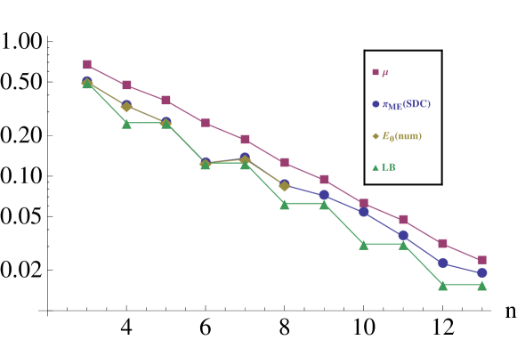
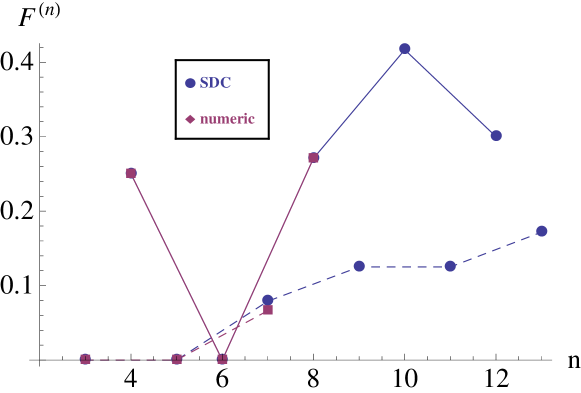
Figure 2 displays the (normalized) difference between the minimum average purity, computed according to Scott’s extremal additive self-dual codes and/or our best numerical estimate, and the lower bound $1/N_{A}$ in Eq. (24). This difference is an upper bound to the frustration ratio

$$F^{(n)}=\frac{E_{0}^{(n)}-1/N_{A}}{E_{0}^{(n)}},\qquad N_{A}=2^{[n/2]},$$ (26)

that can be viewed as the “amount of frustration” in the system. We notice the very different behavior between odd and even values of $n$. In the former case the amount of frustration increases with the size of the system. On the contrary, in the latter case, the behavior is not monotonic. It would be of great interest to understand how this quantity behaves in the thermodynamical limit, but our data do not enable us to draw any clear-cut conclusions.

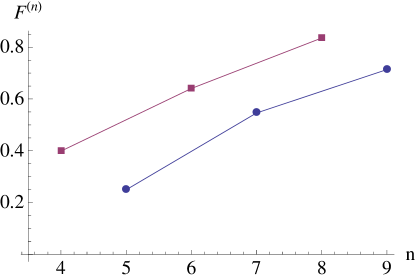
Let us extend these considerations to the continuous variables scenario. In order to measure the amount of frustration (for states belonging to the constrained set $\mathcal{C}$) we define a more general frustration ratio

$$F^{(n),\mathcal{C}}=\frac{E_{0}^{(n),\mathcal{C}}-\pi_{\mathrm{min}}^{[n/2],\mathcal{C}}}{E_{0}^{(n),\mathcal{C}}}$$ (27)

and eventually take the limit $\mathcal{C}\rightarrow\mathcal{H}$, where both the numerator denominator can vanish. [Notice that (26) is a specialization of the quantity in (27) to the qubit case, i.e. $\mathcal{C}=\mathcal{H}=(\mathbb{C}^{2})^{\otimes n}$.] As a constraint we fix the value $\mathcal{N}$ of the average number of excitations per mode, namely

$$\mathcal{C}=\{\psi\in\mathcal{H},\psi\;\mathrm{Gaussian},\frac{\langle q_{k}^{2}+p_{k}^{2}\rangle}{2}\leq\mathcal{N}+\frac{1}{2},1\leq k\leq n\}.$$ (28)

The ideal lower bound is given by [28]

$$\pi_{\mathrm{min}}^{[n/2],\mathcal{C}}=\frac{1}{2^{[n/2]}(\mathcal{N}+1/2)^{[n/2]}}$$ (29)

and represents the purity of a Gaussian thermal state. Incidentally, we notice that, for $\mathcal{N}=1/2$, Eq. (29) reproduces the lower bound of Eq. (14) i. e. the case of qubits. On the other hand, $\mathcal{N}=0$ corresponds to the case of completely separable states. In Fig.  3 we plot the frustration ratio (27) as a function of the number of modes. Each point has been numerically obtained by relaxing the energy constraint ($\mathcal{N}\rightarrow+\infty$) until the ratio $F^{(n),\mathcal{C}}$ has reached a saturation value $F^{(n)}$ [28]. This corresponds to the limit $\mathcal{C}\to\mathcal{H}$.

Figure 2: (Color online) Qubits: frustration ratio: (normalized) distance between the average purity $\pi_{\mathrm{ME}}(\mathrm{SDC})$, according to Scott’s extremal additive self-dual codes (full circles), or our best numerical estimate for the minimum $E_{0}(\mathrm{num})$ (squares), and the lower bound LB=$1/N_{A}$, vs the number of spins. Notice the difference between even and odd $n$.

Figure 3: (Color online) Gaussian states: frustration ratio for and odd (rectangle) and even (circle) number of modes. As explained in the text, each point has been obtained in the saturation regime $\mathcal{C}\to\mathcal{H}$.

3.1 The structure of frustration

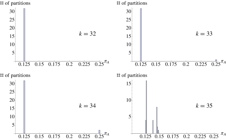
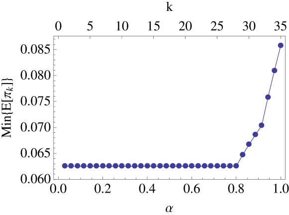
In order to try and understand the underlying structure of this frustration, we focus again on qubits and analyze the behavior of the minimum value of the average purity when one requires the condition (23) for an increasing number of bipartitions. We proceed as follows: we set $n=7$, so that the total number of balanced bipartitions is $K=35$, and add bipartitions one by one, by choosing them so that condition (23) be valid, as far as this is possible. When (23) becomes impossible to satisfy, we require that the average purity be minimal. We plot the minimum average purity as a function of $k$ and $\alpha=k/K$ in Fig. 4 . One observes that it is possible to saturate the minimum $1/N_{A}=1/8=0.125$ up to $k=32$ well chosen partitions. For $k=33$ all bipartitions yield the minimum 1/8, except the last one, that yields 1/4: frustration appears. For $k=34$, two bipartitions yield 1/4. For $k=K=35$ purity is larger than 1/8 for all bipartitions. Notice that the solution with 32 bipartitions at 1/8 and the remaining three at 1/4 corresponds to Scott’s extremal additive self-dual code and would yield a higher average. The distribution of purity for an increasing number of partitions is shown in Fig. 5.

The case $n=8$ is slightly different: see Fig. 6. In this case $K=35$ again and there is no frustration up to $k=28$ bipartitions ($\alpha=0.8$), if properly chosen (all of them with a purity $1/16$). When $k$ is further increased, it is no longer possible to reach the lower bound: for $29\leq k\leq 32$ the new bipartitions have purity $1/8$. Finally, for $33\leq k\leq 35=K$, the new bipartitions have purity $1/4$.

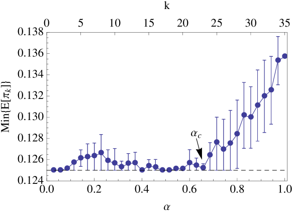
Another useful test is the extraction of $k$ randomly selected bipartitions and the successive minimization of the average purity. This is a typical test in frustrated systems, e.g. in random [43] and Bethe lattices [44]. In this way one checks the onset of frustration independently of the particular choice of the sequence of bipartitions. In Fig. 7 we plot the dependence on $k$ and $\alpha$. Each point corresponds to the extraction of a number of $k$ bipartitions ranging from few tens to a few hundreds. Frustration appears at rather large values of $k$, qualitatively confirming the result shown in Fig. 4. Moreover we notice that for smaller $k$ it is sometimes difficult to reach the minimum. This could be an indicator that for a small number of bipartitions there is a large number of local minima in the energy landscape, that “traps” the numerical procedure. Notice that the curve in Fig.  7 should monotonically increase as a function of $k$, so that all deviations from monotonicity are ascribable to the numerical procedure, and are a consequence of the fact that for different values of $k$, in each run of the simulation, the subset of extracted bipartitions is uncorrelated to the set used for the preceding values of $k$.

Although the results of this section are not conclusive, they provide a clear picture of the relationship between entanglement and frustration. The latter tends to grow with the size of the system (Figs. 2 and 3) and it is difficult to study, at least for small values of $n$, because it suddenly appears at the last few bipartitions (Fig. 4). One estimates, from the results for $n=7$ qubits in Fig. 7, an average fraction of frustrated bipartitions $1-\alpha_{c}\simeq 34\%$, $\alpha_{c}$ being a critical ratio.

A posteriori, it is not surprising that multipartite entanglement, being a complex phenomenon, exhibits frustration. It would be of great interest to understand what happens for larger values of $n$. Different scenarios are possible, according to the mutual interplay between the quantities $F$ and $\alpha_{c}$. In particular, the amount of frustration $F$ shows a tendency to increase with $n$, for both qubit and Gaussian states. This could be ascribable to a decrease of $\alpha_{c}$, corresponding to an increasing fraction of frustrated partitions, or to a constant (or even increasing) $\alpha_{c}$, corresponding to a constant (or decreasing) fraction of increasingly frustrated bipartitions.

Figure 4: (Color online) Minimum average purity for $n=7$ and an increasing number $k$ of bipartitions. Until $k=32$ no frustration appears. For $k=33$ one partition has purity $\pi=1/4$. For $k=34$, two bipartitions yield $\pi=1/4$. For $k=K=35$, $\pi>1/8$ for all bipartitions. $\alpha=k/K$. See Fig. 5.

Figure 5: (Color online) Distribution of purity for $n=7$ and an increasing number $k$ of bipartitions. See Fig. 4.

Figure 6: (Color online) Minimum average purity for $n=8$ and an increasing number $k$ of bipartitions. Until $k=28$ no frustration appears. $\alpha=k/K$.

Figure 7: (Color online) Minimum average purity for $n=7$ and an increasing number $k$ of randomly selected bipartitions. Every point corresponds to an average over different extractions of $k$ bipartitions. The bars correspond to 68% of the distribution (that can be very asymmetric due to the closeness of the lower bound). $\alpha=k/K$. The average fraction of frustrated bipartitions is $1-\alpha_{c}\simeq 34\%$.

4 Concluding remarks

One important property that we have not investigated here and that is often used to characterize multipartite entanglement is the so-called monogamy of entanglement [14, 45], that essentially states that entanglement cannot be freely shared among the parties. Interestingly, although monogamy is a typical property of multipartite entanglement, it is expressed in terms of a bound on a sum of bipartite entanglement measures. This is reminiscent of the approach taken in this paper. The curious fact that bipartite sharing of entanglement is bounded might have interesting consequences in the present context. It would be worth understanding whether monogamy of entanglement generates frustration.

Two crucial issues must be elucidated. First, the striking similarities and small differences between qubits and Gaussian MMES: see Table 1 and compare Figs.  2 and 3. Second, the features of MMES for $n\to\infty$. Finally, we think that the characterization of multipartite entanglement investigated here can be important for the analysis of the entanglement features of many-body systems, such as spin systems and systems close to criticality.

References

- [1] Freud S 1921 in Types of Onset and Neurosis. The Standard Edition of the Complete Psychological Works of Sigmund Freud (Strachey J, The Hogarth Press and the Institute of Psycho-analysis, London, 1958) XII 227.
- [2] Barker R 1938 Character and Personality 7 145.
- [3] Ehlert A 2001 the bullet“iln” 1 2.
- [4] Defined by Lord Radcliffe 1956 in Davis Contractors Ltd v Fareham Urban District Council [1956] AC 696 at 729 and adopted by the High Court of Australia in Codelfa Construction Pty. Ltd. v. State Rail Authority of NSW (1982) 149 CLR 337 at [1956] A.C. p729.
- [5] Mezard M, Parisi G and Virasoro M A, 1987 Spin Glass Theory and Beyond (World Scientific, Singapore).
- [6] Einstein A, Podolsky B and Rosen N 1935 Phys. Rev. 47 777.
- [7] Schrödinger E 1935 Proc. Cambridge Phil. Soc. 31 555.
- [8] Schrödinger E 1936 Proc. Cambridge Phil. Soc. 32 446.
- [9] Wootters W K 2001 Quantum Inf. and Comp. 1 27.
- [10] Amico L, Fazio R, Osterloh A and Vedral V 2008 Rev. Mod. Phys. 80 517.
- [11] Horodecki R, Horodecki P, Horodecki M and Horodecki K 2009 Rev. Mod. Phys. 81, 865.
- [12] Wootters, W K 1998 Phys. Rev. Lett. 80 2245.
- [13] Bennett C H, DiVincenzo D P, Smolin J A and Wootters W K 1996 Phys. Rev. A 54 3824.
- [14] Coffman V, Kundu J and Wootters W K 2000 Phys. Rev. A 61 052306.
- [15] Wong A and Christensen N 2001 Phys. Rev. A 63 044301.
- [16] Bruss D 2002 J. Math. Phys. 43 4237.
- [17] Meyer D A and Wallach N R 2002 J. Math. Phys. 43, 4273.
- [18] Jakob M and Bergou J 2007 Phys. Rev. A 76 052107.
- [19] Man’ko V I, Marmo G, Sudarshan E C G and Zaccaria F 2002 J. Phys. A: Math. Gen. 35 7137.
- [20] Facchi P, Florio G, Marzolino U, Parisi G and Pascazio S 2009 J. Phys. A: Math. Theor. 42 055304.
- [21] Facchi P, Florio G and Pascazio S 2006 Phys. Rev. A 74 04233; 2007 Int. J. Quantum Inf. 5 97.
- [22] Facchi P, Florio G, Parisi G and Pascazio S 2008 Phys. Rev. A 77 060304(R).
- [23] Facchi P 2008 Rend. Lincei Mat. Appl. 2009 20 25.
- [24] Wolf M M, Verstraete F and Cirac J I 2003 Int. J. of Quant. Inf. 1, 465.
- [25] Wolf M M, Verstraete F and Cirac J I 2004 Phys. Rev. Lett. 92, 087903.
- [26] Dawson C M and Nielsen M A 2004 Phys. Rev. A 69, 052316.
- [27] J. Zhang, G. Adesso, C. Xie and K. Peng, Phys. Rev. Lett. 103, 070501 (2009).
- [28] Facchi P, Florio G, Lupo C, Mancini S and Pascazio S 2009 arXiv:0908.0114 [quant-ph].
- [29] Scott A J 2004 Phys. Rev. A 69 052330.
- [30] Parthasarathy K R 2004 Proc. Indian Acad. Sciences 114 365.
- [31] Greenberger D M, Horne M and Zeilinger A 1990 Am. J. Phys. 58 1131.
- [32] Higuchi A and Sudbery A 2000 Phys. Lett. A 273 213.
- [33] Brown I D K, Stepney S, Sudbery A, and Braunstein 2005 J. Phys. A: Math. Gen. 38 1119.
- [34] Brierley S and Higuchi A 2007 J. Phys. A: Math. Gen. 40 8455.
- [35] Braunstein S L and Pati A K 2003 Quantum Information with Continuous Variables (Springer, Berlin).
- [36] Cerf N J, Leuchs G and Polzik E S 2007 Quantum Information with Continuous Variables of Atoms and Light (Imperial College Press, London).
- [37] Lubkin E 1978 J. Math. Phys. 19 1028.
- [38] Lloyd S and Pagels H 1988 Ann. Phys. NY 188 186.
- [39] Page D N 1993 Phys. Rev. Lett. 71 1291.
- [40] Życzkowski K and Sommers H J 2001 J. Phys. A 34 7111.
- [41] Scott A J and Caves C M 2003 J. Phys. A: Math. Gen. 36 9553.
- [42] Giraud O 2007 J. Phys. A: Math. Theor. 40 2793.
- [43] De Dominicis C and Giardina I 2006 Random Fields and Spin Glasses (Cambridge University Press)
- [44] Mezard M and Parisi G 2001 Eur. Phys. J. B 20 217.
- [45] Kim J S, Das A and Sanders B C 2009 Phys. Rev. A 79 012329.