Astrometry.net:
Blind astrometric calibration of arbitrary astronomical images

Abstract

We have built a reliable and robust system that takes as input an astronomical image, and returns as output the pointing, scale, and orientation of that image (the astrometric calibration or WCS information). The system requires no first guess, and works with the information in the image pixels alone; that is, the problem is a generalization of the “lost in space” problem in which nothing—not even the image scale—is known. After robust source detection is performed in the input image, asterisms (sets of four or five stars) are geometrically hashed and compared to pre-indexed hashes to generate hypotheses about the astrometric calibration. A hypothesis is only accepted as true if it passes a Bayesian decision theory test against a null hypothesis. With indices built from the USNO-B Catalog and designed for uniformity of coverage and redundancy, the success rate is $>99.9~{}\!\%$ for contemporary near-ultraviolet and visual imaging survey data, with no false positives. The failure rate is consistent with the incompleteness of the USNO-B Catalog; augmentation with indices built from the 2MASS Catalog brings the completeness to $100~{}\!\%$ with no false positives. We are using this system to generate consistent and standards-compliant meta-data for digital and digitized imaging from plate repositories, automated observatories, individual scientific investigators, and hobbyists. This is the first step in a program of making it possible to trust calibration meta-data for astronomical data of arbitrary provenance.

1 Introduction

Although there are hundreds of ground- and space-based telescopes currently operating, and petabytes of stored astronomical images (some fraction of which are available in public archives), most astronomical research is conducted using data from a single telescope. Why do we as astronomers limit ourselves to using only small subsets of the enormous bulk of available data? Three main reasons can be identified: we don’t want to share our data; it’s hard to share our data; and it’s hard to use data that others have shared. The latter two problems can be addressed by technological solutions, and as sharing data becomes easier, astronomers will likely become more willing to do so.

Historically, astronomical data—and, indeed, important scientific results—have often been closely guarded. In more recent times, early access to data has been seen as one of the rewards for joining and contributing to telescope-building collaborations, and proprietary data periods typically accompany grants of observing time on observatories such as the Hubble Space Telescope. However, this seems to be changing, albeit slowly. One of the first large astronomical data sets to be released publicly in a usable form was the Hubble Deep Field (Williams et al., 1996). The Sloan Digital Sky Survey (SDSS; York et al. 2000) is committed to yearly public data releases, and the members of upcoming projects such as the Large Synoptic Survey Telescope (LSST; Ivezic et al. 2008) have recognized that the primary advantage of contributing to the collaboration is not proprietary access to the data, but rather a deep understanding and familiarity with the telescope and data, and have (in principle) decided to make the data available immediately.

Putting aside the issue of willingness to share data, there are issues of our ability to share data effectively. Making use of large, heterogeneous, distributed image collections requires fast, robust, automated tools for calibration, vetting, organization, search and retrieval.

The Virtual Observatory (VO; Szalay 2001) establishes a framework and protocols for the organization, search, and retrieval of astronomical images. The VO is structured as a distributed system in which many “publishers” provide image collections and interfaces that allow these images to be searched. This distributed framework allows the VO to scale, but it also means that any property we might want the images published through the VO to have must be specified by the standards, and we must trust all publishers to implement the standards correctly. Of particular importance are calibration meta-data (Schade, 2005). The draft Simple Image Access Protocol (Tody & Plante, 2009) states that “an image should be a calibrated object frame” and specifies some loose requirements for astrometric meta-data. However, there is neither a requirement, nor a specified method, for communicating more detailed information about the calibration processes that have been applied to the image. A VO user who wants to know exactly how the raw CCD frame was reduced to the pixel values in the image must use processes outside the VO framework—most likely by reading papers and contacting the image publisher—and this will take much longer than finding and retrieving the image.

The VO cannot be expected to impose a minimum standard of “quality” on images published through VO protocols, for several reasons. First, doing so would require making a tradeoff between the quality and quantity of images that are publishable. Since different users of the VO have different needs, there is no objective way to make this tradeoff. For example, one researcher might only want images taken during photometric conditions, while one studying a transient event might want all available imaging, regardless of quality. Second, there is no objective measure of the quality of an image: different aspects of an image are important to different users. Finally, even the most well-intentioned and skilled publisher will occasionally make mistakes, and this effect will become more pronounced as surveys become more automated and data rates increase. Thus, users of the VO cannot in general rely on the quality or correctness of image data or calibration meta-data, and individually hand-checking each image does not scale to the future in which the VO provides access to any significant fraction of the world’s astronomical images. For the goals of the VO movement to be achieved, the tools that allow users to vet, verify, and recalibrate images must be developed, and ideally these tools will be integrated into the VO system.

In this article we present a system, Astrometry.net, that automatically produces astrometric meta-data for astronomical images. That is, given an image, our system produces the pointing, scale, and orientation of the image—the astrometric calibration meta-data or World Coordinate System (WCS). The system requires no first guess, and works with the information in the image pixels alone. The success rate is above $99.9~{}\!\%$ for contemporary near-ultraviolet and visual imaging survey data, with no false positives.

Our system enables an immense amount of “lost” astronomical imagery to be used for scientific purposes. This includes photographic plate archives, an immense and growing number of images taken by amateur astronomers, as well as data from individual professional astronomers and ground-based observatories whose meta-data are non-existent, lost, or simply wrong. While many modern telescopes do produce correct, standards-compliant meta-data, many others have control systems that drift relative to the sky, yielding only approximate astrometric meta-data. Still others produce no meta-data, or produce it in some ideosyncratic, non-standards-compliant form. Even sophisticated and highly-automated surveys such as SDSS occasionally have failures in the systems that produce astrometric calibration information, resulting in perfectly good but “lost” images. A system that makes these data available for study will effectively recover a significant amount of lost observing time, fill in gaps in the astronomical record, and make observers more productive by eliminating the tedious and often unenlightening task of fixing the astrometry. Furthermore, a robust, fully-automated system allows the data to be trusted, because the calibration meta-data, and their associated error estimates, have been derived from the images themselves, not from some unknown, undocumented, unverified or untrustworthy external source.

Our system can be seen as a specialized kind of image-based search. Given an image, we can identify and label the objects that appear in the image, with a very high success rate and no false positives. We have achieved the ultimate goal of computer vision, within the domain of astronomical images. Our system is based solely on the contents of the image, in sharp contrast to most contemporary image search systems (such as Google Image Search), which rely on contextual information—the text surrounding the image on a web page—rather than the information in the image itself.

In the literature, the task of recognizing astronomical images is known as “blind astrometric calibration” or the “lost in space” problem, since an early application was for estimating the attitude of a spacecraft using a camera mounted on the spacecraft. By identifying the stars that are visible, the pose of the camera can be determined (Liebe, 1993). In such systems, triangles of stars are typically used as geometric features (for example, Junkins et al. 1977). Triangles are effective in this regime because the images typically span tens of degrees and contain only dozens of very bright stars: the search space is small. Furthermore, these systems are not fully “blind” in that they are designed for particular cameras, the specifications of which are available to the system designers.

Triangle-based approaches have also been used to fine-tune the astrometry problem when a good initial estimate is available (Pál & Bakos, 2006). Because the search domain is limited to a small area around the initial estimate, the triangle-based approach is effective. Completely blind systems have been attempted previously (for example, Harvey 2004 and references therein) but none we know of have been able to achieve the scalability and fidelity of our approach.

Both the triangle matching approach and ours (described below) are based on “geometric hashing” (for example, Lamdan et al. 1990, Huttenlocher & Ullman 1990). Our system uses the same two-step approach used by these systems, in which a set of hypotheses are generated from sparse matches, then a second stage does detailed verification of the hypotheses.

There are several automated calibration systems that refine the astrometric calibration of an image to produce a high-precision alignment to a reference catalog given a good first guess (for example, Valdes et al. 1995; Mink 2006; Bertin 2005). These systems are reliable and robust, but they require a reasonable first guess about the image pointing, orientation, and scale. Our system can be used to create that good first guess.

2 Methods

Our approach involves four main components. First, when given a query image, we detect astronomical sources (“stars”, hereafter) by running a number of image-processing steps. This typically yields a few hundred or more stars localized to sub-pixel accuracy. Next, the system examines subsets of these stars, producing for each subset a geometric hash code that describes their relative positions. We typically use subsets of four stars, which we call “quads.” Having computed the hash code for the query quad, the system then searches in a large pre-computed index for almost identical hash codes. Each matching hash code that is found corresponds to a hypothesized alignment between the quad in the query image and the quad in the index, which can be expressed as a hypothesized location, scale, and orientation of the image on the sky. The final component is a verification criterion, phrased as a Bayesian decision problem, which can very accurately decide if the hypothesized alignment is correct. The system continues generating and testing hypotheses until we find one that is accepted by the verification process; we then output that hypothesis as our chosen alignment. In some cases, we never find a hypothesis in which we are sufficiently confident (or we give up searching before we find one), but our thresholds are set conservatively enough that we almost never produce a false positive match. Each component of our approach is outlined below.

The primary technical contributions of our system include the use of the “geometric hashing” (Lamdan et al., 1990; Wolfson & Rigoutsos, 1997) approach to solve the huge search problem of generating candidate calibrations; an index-building strategy that takes into account the distribution of images we wish to calibrate; the verification procedure which determines whether a proposed astrometric calibration is correct; and good software engineering which has allowed us to produce a practical, efficient system. All our code is publicly available under the GPL license, and we are also offering a web service.

2.1 Star detection

The system automatically detects compact objects in each input image and centroids them to yield the pixel-space locations of stars. This problem is an old one in astronomy; the challenge here is to perform it robustly, with no human intervention, on the large variety of input images the system faces. Luckily, because the rest of the system is so robust, it can handle detection lists that are missing a few stars or have some contaminants.

The first task is to identify (detect) localized sources of light in the image. Most astronomical images exhibit sky variations, sensitivity variations, and scattering; we need to find peaks on top of such variations. First we subtract off a median-smoothed version of the image to “flatten” it. Next, to find statistically significant peaks, we need to know the approximate noise level. We find this by choosing a few thousand random pairs of pixels separated by five rows and columns, calculating the difference in the fluxes for each pair, and calculating the variance of those differences, which is approximately twice the variance $\sigma^{2}$ in each pixel. At this point, we identify pixels which have values in the flattened image that are $>8\,\sigma$, and connect detected pixels into individual detected objects.

The second task is to find the peak or peaks in each detected object. This determination begins by identifying pixels that contain larger values than all of their neighbors. However, keeping all such pixels would retain peaks that are just due to uncorrelated noise in the image and individual peaks within a single “object.” To clean the peak list, we look for peaks that are joined to smaller peaks by saddle points within $3\,\sigma$ of the larger peak (or $1~{}\!\%$ of the larger peak’s value, whichever is greater), and trim the smaller peaks out of our list.

Finally, given the list of all peaks, the third task is to centroid the star position at sub-pixel accuracy. Following previous work (Lupton et al., 2001), we take a $3\times 3$ grid around each star’s peak pixel, effectively fitting a Gaussian model to the nine values, and using the peak of the Gaussian. Occasionally this procedure produces a Gaussian peak outside the $3\times 3$ grid, in which case we default to the peak pixel, although such cases are virtually always caused by image artifacts. This procedure produces a set of $x$ and $y$ positions in pixel coordinates corresponding to the position of objects in the image.

Compared to other star detection systems such as SExtractor (Bertin & Arnouts, 1996), our approach is simpler and generally more robust given a wide variety of images and no human intervention. For example, while we do a simple median-filtering to remove the background signal from the image, SExtractor uses sigma-clipping and mode estimation on a grid of subimages, which are then median-filtered and spline-interpolated.

2.2 Hashing of asterisms to generate hypotheses

Hypotheses about the location of an astronomical image live in the continuous four-dimensional space of position on the celestial sphere (pointing of the camera’s optical axis), orientation (rotation of the camera around its axis), and field of view (solid angle subtended by the camera image). We want to be able to recognize images that span less than one-millionth the area of the sky, so the effective number of hypotheses is large; exhaustive search will be impractical. We need a fast search heuristic: a method for proposing hypotheses that almost always proposes a correct hypothesis early enough that we have the resources to discover it.

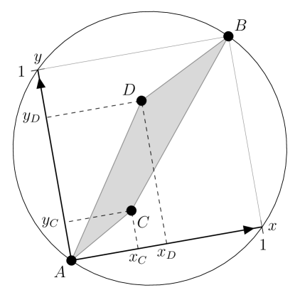
Figure 1: The geometric hash code for a “quad” of stars, $A$, $B$, $C$, and $D$. Stars $A$ and $B$ define the origin and $(1,1)$, respectively, of a local coordinate system, in which the positions of stars $C$ and $D$ are computed. The coordinates $(x_{C},y_{C},x_{D},y_{D})$ become our geometric hash code that describes the relative positions of the four stars. The hash code is invariant under translation, scaling, and rotation of the four stars.

Our fast search heuristic uses a continuous geometric hashing approach. Given a set of stars (a “quad”), we compute a local description of the shape—a geometric hash code—by mapping the relative positions of the stars in the quad into a point in a continuous-valued, 4-dimensional vector space (“code space”). Figure 1 shows this process. Of the four stars comprising the quad, the most widely-separated pair are used to define a local coordinate system, and the positions of the remaining two stars in this coordinate system serve as the hash code. We label the most widely-separated pair of stars “$A$” and “$B$”. These two stars define a local coordinate system. The remaining two stars are called “$C$” and “$D$”, and their positions in this local coordinate system are $(x_{C},y_{C})$ and $(x_{D},y_{D})$. The geometric hash code is simply the 4-vector $(x_{C},y_{C},x_{D},y_{D})$. We require stars $C$ and $D$ to be within the circle that has stars $A$ and $B$ on its diameter. This hash code has some symmetries: swapping $A$ and $B$ converts the code to $(1\!-\!x_{C},1\!-\!y_{C},1\!-\!x_{D},1\!-\!y_{D})$ while swapping $C$ and $D$ converts $(x_{C},y_{C},x_{D},y_{D})$ into $(x_{D},y_{D},x_{C},y_{C})$. In practice, we break this symmetry by demanding that $x_{C}\leq x_{D}$ and that $x_{C}+x_{D}\leq 1$; we consider only the permutation (or relabelling) of stars that satisfies these conditions (within noise tolerance).

This mapping has several properties that make it well suited to our indexing application. First, the code vector is invariant to translation, rotation and scaling of the star positions so that it can be computed using only the relative positions of the four stars in any conformal coordinate system (including pixel coordinates in a query image). Second, the mapping is smooth: small changes in the relative positions of any of the stars result in small changes to the components of the code vector; this makes the codes resilient to small amounts of positional noise in star positions. Third, if stars are uniformly distributed on the sky (at the angular scale of the quads being indexed), codes will be uniformly distributed in (and thus make good use of) the 4-dimensional code-space volume.

Noise in the image and distortion caused by the atmosphere and telescope optics lead to noise in the measured positions of stars in the image. In general this noise causes the stars in a quad to move slightly with respect to each other, which yields small changes in the hash code (i.e., position in code space) of the quad. Therefore, we must always match the image hash code with a neighborhood of hash codes in the index.

The standard geometric hashing “recipe” would suggest using triangles rather than quads. However, the positional noise level in typical astronomical images is sufficiently high that triangles are not distinctive enough to yield reasonable performance. An important factor in the performance of geometric hashing system is the “oversubscription factor” of code space. The number of hash codes that must be contained in an index is determined by the effective number of objects that are to be recognized by the system: if the goal is to recognize a million distinct objects, the index must contain at least a million hash codes. Each hash code effectively occupies a volume in code space: since hash codes can vary slightly due to positional noise in the inputs (star positions), we must always search for matching codes within a volume of code space. This volume is determined by the positional noise levels in the input image and the reference catalog. The oversubscription factor of code space, if it is uniformly populated, is simply the number of codes in the index multiplied by the fractional volume of code space occupied by each code. If triangles are used, the fractional volume of code space occupied by a single code is large, so the code space becomes heavily oversubscribed. Any query will match many codes by coincidence, and the system will have to reject all of these false matches, which is computationally expensive. By using quads instead of triangles, we nearly square the distinctiveness of our features: a quad can be thought of as two triangles that share a common edge, so a quad essentially describes the co-occurrence of two triangles. A much smaller fraction of code space is occupied by each quad, so we expect fewer coincidental (false) matches for any given query, and therefore fewer false hypotheses which must be rejected.

We could use quintuples of stars, which are even more distinctive than quads. However, there are two disadvantages to increasing the number of stars in our asterisms. The first is that the probability that all $k$ of the stars in an indexed asterism appear in the image and that all $k$ of the stars in a query asterism appear in the index both decrease with increasing $k$. For images taken at wavelengths far from the catalog wavelength, or shallow images, this consideration can become severe. The second disadvantage is that near-neighbor lookup, even with a kd-tree, becomes more time-consuming with increasing dimensionality. The dimensionality of the code space for quintuples is $6$-dimensional, compared to the $4$-dimensional code space of quads. We test triangle- and quintuple-based indices in section 3.1.7 below.

When presented with a list of stars from an image to calibrate, the system iterates through groups of four stars, treating each group as a quad and computing its hash code. Using the computed code, we perform a neighborhood lookup in the index, retrieving all the indexed codes that are close to the query code, along with their corresponding locations on the sky. Each retrieved code is effectively a hypothesis, which proposes to identify the four reference catalog stars used to create the code at indexing time with the four stars used to compute the query code. Each such hypothesis is evaluated as described below.

The question of which hypotheses to check and when to check them is a purely heuristic one. One could chose to wait until a hypothesis has two or more “votes” from independent codes before checking it or check every hypothesis as soon as it is proposed, whichever is faster. In our experiments, we find that it is faster, and much less memory-intensive, to simply check every hypothesis rather than accumulate votes.

2.3 Indexing the sky

As with all geometric hashing systems, our system is based around a pre-computed index of known asterisms. Building the index begins with a reference catalog of stars. We typically use an all-sky (or near-all-sky) optical survey such as USNO-B1 (Monet et al., 2003; Barron et al., 2008) as our reference catalog, but we have also used the infrared 2MASS catalog (Skrutskie et al., 2006) and the ultraviolet catalog from GALEX (Martin & GALEX Science Team, 2003), as well as non-all-sky catalogs such as SDSS. From the reference catalog we select a large number of quads (using a process described below). For each quad, we store its hash code and a reference to the four stars of which it is composed. We also store the positions of those four stars. Given a query quad, we compute its hash code and search for nearby codes in the index. For each nearby code, we look up the corresponding four stars in the index, and create the hypothesis that the four stars in the query quad correspond to the four stars in the index. By looking up the positions of the query stars in image coordinates and the index stars in celestial coordinates, we can express the hypothesis as a pointing, scale, and rotation of the image on the sky.

In order for our approach to be successful, our index must balance several properties. We want to be able to recognize images from any part of the sky, so we want to choose quads uniformly over the sky. We want to be able to recognize images with a wide range of angular sizes, so we want to choose quads of a variety of sizes. We expect that brighter stars will be more likely to be found in our query images, so we want to build quads out of bright stars preferentially. However, we also expect that some stars, even the brightest stars, will be missing or mis-detected in the query image (or the reference catalog), so we want to avoid over-using any particular star to build quads.

We handle the wide range of angular sizes by building a series of sub-indices, each of which contains quads whose quads have scales within a small range (for example, a factor of two). At some level this is simply an implementation detail: we could recombine the sub-indices into a single index, but in what follows it is helpful to be able to assume that the sub-index will be asked to recognize query images whose angular sizes are similar to the size of the quads it contains. Since we have a set of sub-indices, each of which is tuned to an overlapping range of scales, we know that at least one will be tuned to the scale of the query image.

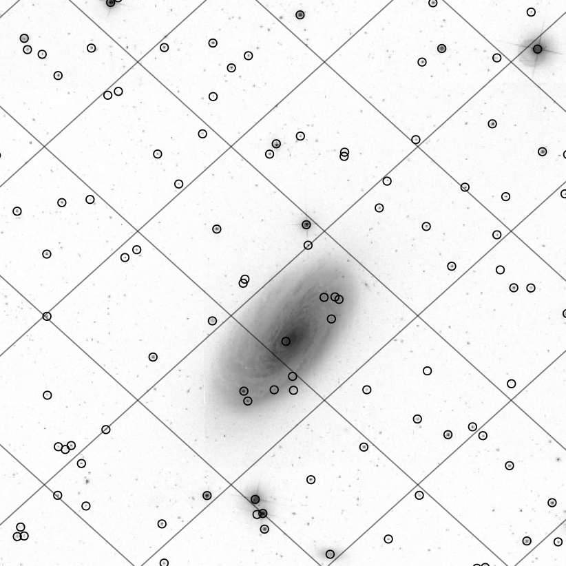
Figure 2: A small region of sky (about $0.3\times 0.3~{}\mathrm{degrees}$ centered on $(\mathrm{RA},\mathrm{Dec})=(188,14.45)~{}\mathrm{degrees}$), showing the HEALPix grid, and the brightest $5$ stars that we select from each cell. The image shown is from the Sloan Digital Sky Survey.

We begin by selecting a spatially-uniform and bright subset of stars from our reference catalog. We do this by placing a grid of equal-area patches (“HEALPixels”; Górski et al. 2002) over the sky and selecting a fixed number of stars, ordered by brightness, from each grid cell. The grid size is chosen so that grid cells are a small factor smaller than the query images. Typically we choose the grid cells to be about a third of the size of the query images, and select $10$ stars from each grid cell, so that most query images will contain about a hundred query stars. Figure 2 illustrates this process on a small patch of sky.

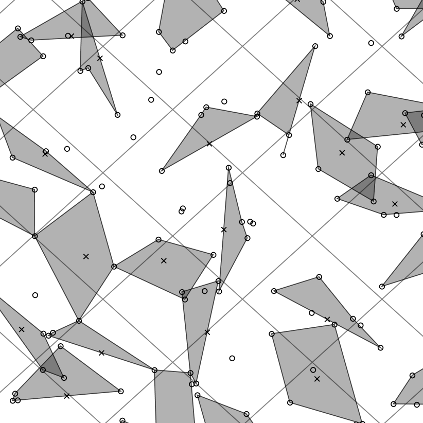
Figure 3: The same region of sky as shown in the previous figure, showing the HEALPix grid, and the quads that are created during the first pass through the grid cells. The quads must have a diameter (the distance between the two most distant stars) within a given range—in this case, $1$ to $\sqrt{2}$ times the side-length of the grid cells. In each grid cell, the system attempts to build a quad whose center (i.e., midpoint of the diameter line)—marked with an $\mathbf{\times}$ in the figure—is within the grid cell.

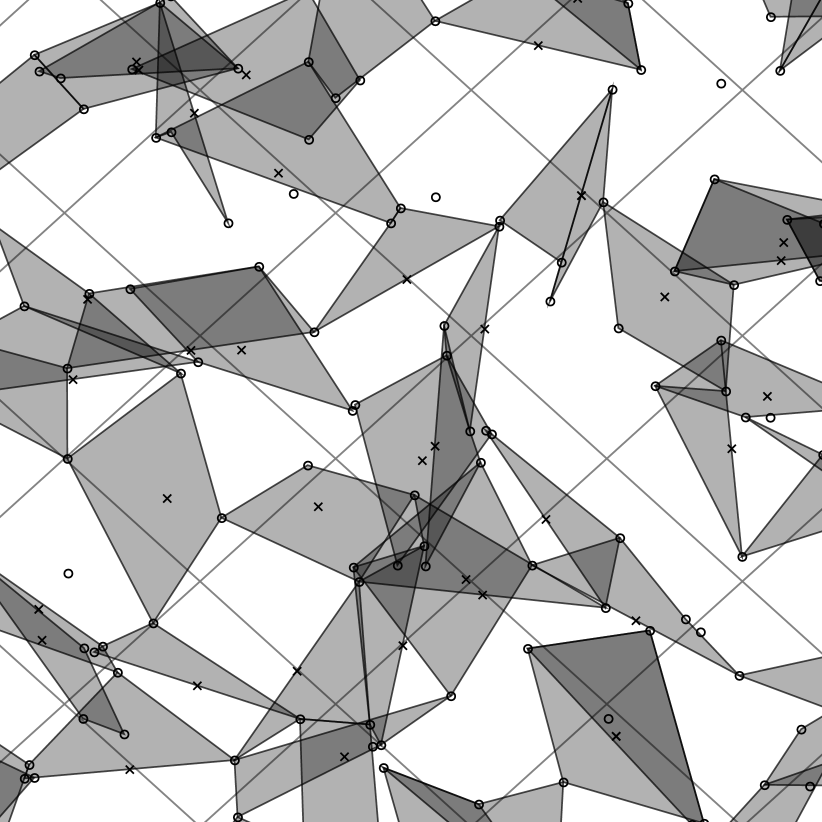
Figure 4: The same region of sky as in the previous figures, showing the quads that are created after the second round of attempting to build a quad in each grid cell.

Next, we visit each grid cell and attempt to find a quad within the acceptable range of angular sizes and whose center lies within the grid cell. We search for quads starting with the brightest stars, but for each star we track the number of times it has already been used to build a quad, and we skip stars that have been used too many times already. We repeat this process, sweeping through the grid cells and attempting to build a quad in each one, a number of times. In some grid cells we will be unable to find an acceptable quad, so after this process has finished we make further passes through the grid cells, removing the restriction on the number of times a star can be used, since it is better to have a quad comprised of over-used stars than no quad at all. Typically we make a total of $16$ passes over the grid cells, and allow each star to be used in up to $8$ quads. Figures 3 and 4 show the quads built during the first two rounds of quad-building in our running example.

In principle, an index is simply a list of quads, where for each quad we store its geometric hash code, and the identities of the four stars of which it is composed (from which we can look up their positions on the sky). However, we want to be able to search quickly for all hash codes near a given query hash code. We therefore organize the hash codes into a kd-tree data structure, which allows rapid retrieval of all quads whose hash codes are in the neighborhood of any given query hash code. In order to carry out the verification step we also keep the star positions in a kd-tree, since for each matched quad we need to find other stars that should appear in the image if the match is true. Since none of the available kd-tree implementations were satisfactory for our purposes, we created a fast, memory-efficient, pointer-free kd-tree implementation (Lang, 2009).

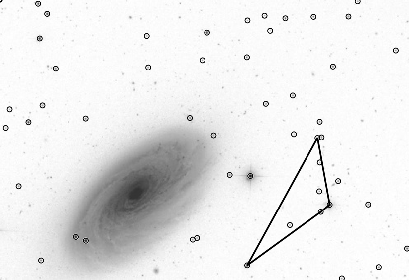
Figure 5: A sample query image, with the brightest $100$ sources our system detects (circles), and a quad in the image to which our system will search for matches in the index. This quad looks like a triangle because two of its stars are nearly collinear. Image credit: Sloan Digital Sky Survey.

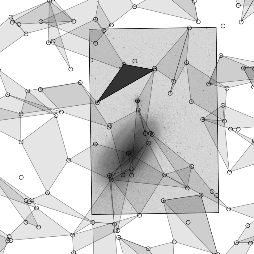
Figure 6: Our example index, showing a quad in the index that matches a quad from the query image (shaded solid). The image is shown projected in its correct orientation on the sky.

Given a query image, we detect stars as discussed above, and sort the stars by brightness. Next, we begin looking at quads of stars in the image. For each quad, we compute its geometric hash code and search for nearby codes in the index. For each matching code, we retrieve the positions of the stars that compose the quad in the index, and compute the hypothesized alignment—the World Coordinate System—of the match. We then retrieve other stars in the index that are within the bounds of the image, and run the verification procedure to determine whether the match is true or false. We stop searching when we find a true match in which we are sufficiently confident, or we exhaust all the possible quads in the query image, or we run out of time. See LABEL:~5.

2.4 Verification of hypotheses

The indexing system generates a large number of hypothesized alignments of the image on the sky. The task of the verification procedure is to reject the large number of false matches that are generated, and accept true matches when they are found. Essentially, we ask, “if this proposed alignment were correct, where else in the image would we expect to find stars?” and if the alignment has very good predictive power, we accept it.

We have framed the verification procedure as a Bayesian decision process. The system can either accept a hypothesized match—in which case the hypothesized alignment is returned to the user—or the system can reject the hypothesis, in which case the indexing system continues searching for matches and generating more hypotheses. In effect, for each hypothesis we are choosing between two models: a “foreground” model, in which the alignment is true, and a “background” model, in which the alignment is false. In Bayesian decision-making, three factors contribute to this decision: the relative abilities of the models to explain the observations, the relative proportions of true and false alignments we expect to see, and the relative costs or utilities of the outcomes resulting from our decision.

The Bayes factor is a quantitative assessment of the relative abilities of the two models—the foreground model $F$ and the background model $B$—to produce or explain the observations. In this case the observations, or data, $D$, are the stars observed in the query image. The Bayes factor

$$K=\frac{p(D\,|\,F)}{p(D\,|\,B)}$$ (1)

is the ratio of the marginal likelihoods. We must also include in our decision-making the prior $p(F)/p(B)$, which is our a priori belief, expressed as a ratio of probabilities, that a proposed alignment is correct. Since we typically examine many more false alignments than true alignments (because we stop after the first true alignment is found), this ratio will be small. We typically set it, conservatively, to $10^{-6}$.

The final component of Bayesian decision theory is the utility table, which expresses the subjective value of each outcome. It is good to accept correctly a true match or reject correctly a false match (“true positive” and “true negative” outcomes, respectively), and it is bad to reject a true match or accept a false match (“false negative” and “false positive” outcomes, respectively). In the Astrometry.net setting, we feel it is very bad to produce a false positive: we would much rather fail to produce a result rather than produce a false result, because we want the system to be be able to run on large data sets without human intervention, and we want to be confident in the results. Our utility table is shown here.

		Reality
		True Alignment		False Alignment
Decision	Accept	$u(\mathrm{TP})=$	$+1$	$u(\mathrm{FP})=$	$-1999$
	Reject	$u(\mathrm{FN})=$	$-1$	$u(\mathrm{TN})=$	$+1$

Applying Bayesian decision theory, we make our decision to accept or reject the hypothesized alignment by computing the expected utility $\mathbb{E}\left[\,u\,\right]$ of each decision. The expected utility of accepting the alignment is:

$$\mathbb{E}\left[\,u\,|\,\mathrm{Accept},D\,\right] =u(\mathrm{TP})\,p(\mathrm{TP}\,|\,D)+u(\mathrm{FP})\,p(\mathrm{FP}\,|\,D)$$ (2)

$$=u(\mathrm{TP})\,p(F\,|\,D)+u(\mathrm{FP})\,p(B\,|\,D)$$ (3)

while the expected utility of rejecting the alignment is:

$$\mathbb{E}\left[\,u\,|\,\mathrm{Reject},D\,\right] =u(\mathrm{FN})\,p(\mathrm{FN}\,|\,D)+u(\mathrm{TN})\,p(\mathrm{TN}\,|\,D)$$ (4)

$$=u(\mathrm{FN})\,p(F\,|\,D)+u(\mathrm{TN})\,p(B\,|\,D)\quad.$$ (5)

We should accept the hypothesized alignment if:

$$\mathbb{E}\left[\,u\,|\,\mathrm{Accept},D\,\right] >\mathbb{E}\left[\,u\,|\,\mathrm{Reject},D\,\right]$$ (6)

$$u(\mathrm{TP})\,p(F\,|\,D)+u(\mathrm{FP})\,p(B\,|\,D) >u(\mathrm{FN})\,p(F\,|\,D)+u(\mathrm{TN})\,p(B\,|\,D)$$ (7)

$$\frac{p(F\,|\,D)}{p(B\,|\,D)} >\frac{u(\mathrm{TN})-u(\mathrm{FP})}{u(\mathrm{TP})-u(\mathrm{FN})}$$ (8)

$$K >\frac{p(B)}{p(F)}\ \frac{u(\mathrm{TN})-u(\mathrm{FP})}{u(\mathrm{TP})-u(\mathrm{FN})}$$ (9)

where we have applied Bayes’ theorem to get

$$\frac{p(F\,|\,D)}{p(B\,|\,D)}=K\ \frac{p(F)}{p(B)}\quad.$$ (10)

With the prior and utilities given above, we find that we should accept a hypothesis if:

$$K >\frac{p(B)}{p(F)}\ \frac{u(\mathrm{TN})-u(\mathrm{FP})}{u(\mathrm{TP})-u(\mathrm{FN})}$$ (11)

$$K >10^{6}\ \frac{1--1999}{1--1}$$ (12)

$$K >10^{9}$$ (13)

That is, we accept a proposed alignment if the Bayes factor of the foreground model to the background model exceeds a threshold that is set based on our desired operating characteristics. In our case, the threshold is large so the foreground model (in which the alignment is true) must be far better at explaining (i.e., predicting) the observed positions of stars in the query image than the background model (in which the alignment is false).

In the foreground model, $F$, the four stars in the query image and the four stars in the index are aligned. We therefore expect that other stars in the query image will be close to other stars in the index. However, we also know that some fraction of the stars in the query image will have no counterpart in the index, due to occlusions or artifacts in the images, errors in star detection or localization, differences in the spectral bandpass, or because the query image “star” is actually a planet, satellite, comet, or some other non-star, non-galaxy object. True stars can be lost, and false stars can be added. Our foreground model is therefore a mixture of a uniform probability that a star will be found anywhere in the image—a query star that has no counterpart in the index—plus a blob of probability around each star in the index, where the size of the blob is determined by the combined positional variances of the index and query stars.

Under the background model, $B$, the proposed alignment is false, so the query image is from some unknown part of the sky; the index is not useful for predicting the positions of stars in the image. Our simple model therefore places uniform probability of finding stars anywhere in the test image. We have experimented with a more sophisticated background models that adapts to the observed distribution of image stars, but we do not discuss that work here.

The verification procedure evaluates stars in the query image, in order of brightness, under the foreground and background models. The product of the foreground-to-background ratios is the Bayes factor. We continue adding query stars until the Bayes factor exceeds our threshold for accepting the match, or we run out of query stars.

3 Results

3.1 Blind astrometric calibration of the Sloan Digital Sky Survey

We explored the potential for automatically organizing and annotating a large real-world data set by taking a sample of images generated by the Sloan Digital Sky Survey and considering them as an unstructured set of independent queries to our system. For each SDSS image, we discarded all meta-data, including all positional and rotational information and the date on which the exposure was taken. We allowed ourselves to look only at the two-dimensional positions of detected “stars” (most of which were in fact stars but some of which were galaxies or detection errors) in the image. Normally, our system would take images as input, running a series of image processing steps to detect stars and localize their positions. The SDSS data reduction pipeline already includes such a process, so for these experiments we used these detected star positions rather than processing all the raw images ourselves. Further experiments have shown that we would likely have achieved similar, if not better, results by using our own image processing software.

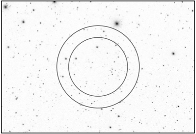
Figure 7: A typical image from the Sloan Digital Sky Survey (SDSS). The range of quad diameters that we use in the experiments below is shown by the circles. Image credit: Sloan Digital Sky Survey.

Each SDSS image has $2048\times 1489$ pixels and covers $9\times 13~{}\mathrm{arcmin}^{2}$, slightly less than one-millionth the area of the sky. Each image measures one of five bandpasses, called $u$, $g$, $r$, $i$, and $z$, spanning the near-infrared through optical to near-ultraviolet range. Each band receives a $54$-second exposure on a $2.5$-meter telescope. A typical image is shown in LABEL:~7.

The SDSS image-processing pipeline assigns to each image a quality rating: “excellent”, “good”, “acceptable”, or “bad”. We retrieved the source positions (i.e., the list of objects detected by the SDSS image-processing pipeline) in every image within the main survey (Legacy and SEGUE footprints), using the public Catalog Archive Server (CAS) interface to Data Release 7 (Abazajian et al., 2009). We retrieved only sources categorized as “primary” or “secondary” detections of stars and galaxies, and required that each image contained at least $300$ objects. The images that are excluded by these cuts contain either very bright stars or peculiarities that cause the SDSS image-processing pipeline to balk. The number of images in Data Release 7 and our cut is given in the table below.

Quality	Total number of images	Number of images in our cut
excellent	$183,359$	$182,221$
good	$101,490$	$100,763$
acceptable	$48,802$	$48,337$
bad	$93,692$	$89,219$
total	$427,343$	$420,540$

3.1.1 Performance on excellent images

In order to show the best performance achievable with our system, we built an index that is well-matched to SDSS $r$-band images. Starting with the red bands from a cleaned version of the USNO-B catalog, we built an index containing stars drawn from a HEALPix grid with cell sizes about $4\times 4~{}\mathrm{arcmin}^{2}$, and $10$ stars per cell. We then built quads with diameters of $4$ to $5.6~{}\mathrm{arcmin}$. For each grid cell, we searched for a quad whose center was within the grid cell, starting with the brightest stars but allowing each star to be used at most $8$ times. We repeated this process $16$ times. The index contains a total of about $100$ million stars and $150$ million quads. Figure 8 shows the spatial distribution of the stars and quads in the index.

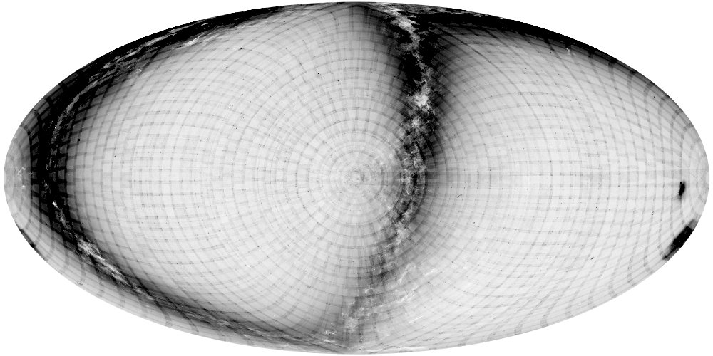
Figure 8: Top: Density of sources in the USNO-B catalog (in Hammer-Aitoff projection). Dark colors indicate high density. The north celestial pole is in the center of the image. The dark strip through the center and around the edges is the Milky Way; lower-density dust lanes can be seen. The USNO-B catalog was created by scanning photographic plates, and the places where the plates overlap are clearly visible as concentric rings and spokes of overdensities. Middle: Density of sources in our spatially uniform cut of the USNO-B catalog. Most of the sky is very uniformly covered. A few small bright (low-density) areas are visible, including a line near the bottom. These are areas where the USNO-B catalog is underdense due to defects. Bottom: Density of quads in the index used in most of the experiments presented here. Again, most of the sky is uniformly covered with quads.

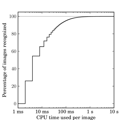
Figure 9: Results from the excellent $r$-band SDSS images and USNO-B-based index. The percentage of images that are recognized correctly (i.e., astrometrically calibrated) with respect to the CPU time spent per image. Many images are recognized rapidly, but there is a heavy tail of “hard” images. Spending more and more CPU results in sharply diminishing returns. After $1$ second, over $99.7~{}\!\%$ of images are recognized, and after $10$ seconds, over $99.97~{}\!\%$ are recognized. The steps are due to the finite resolution of the CPU timer we are using.

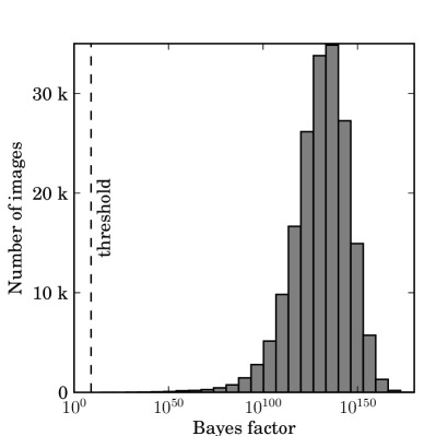
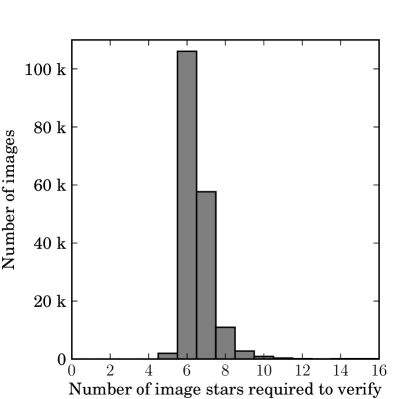
Figure 10: Results from the excellent $r$-band SDSS images, continued. Left: The Bayes factor of the foreground model versus the background model for the hypotheses that we accept. The dashed line shows the threshold implied by our desired operating characteristics. These excellent-quality images yield incredibly high Bayes factors—when we find a correct match is it unequivocal. Right: The number of stars in the query image that had to be examined before the Bayes-factor threshold was reached.

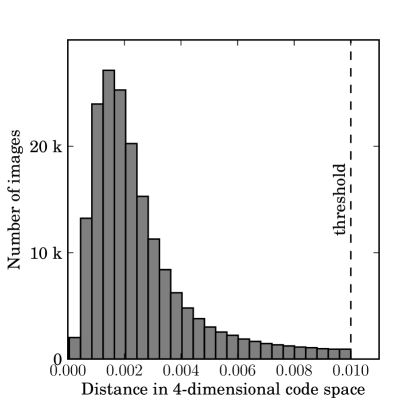
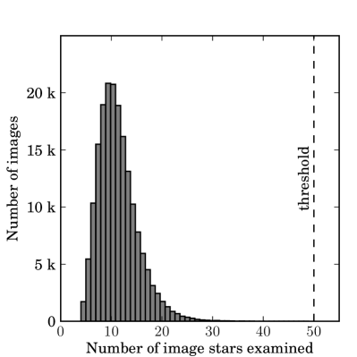
Figure 11: Results from the excellent $r$-band SDSS images, continued. Left: The distance in four-dimensional geometric hash code space between the query quad and the first correctly-matched index quad. In this experiment we searched for matches within distance $0.01$: well into the tail of the distribution. Right: The number of stars in the query image that the system built quads from before finding the first correct match. In a few cases, the brightest $4$ stars formed a valid quad which was matched correctly to the index: we got the correct answer after our first guess!

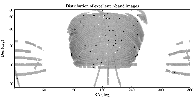
Figure 12: Distribution of the excellent-quality $r$-band SDSS images on the sky. The gray footprint represents the correctly-recognized images, while the black dots show the images that were not recognized using the USNO-B-based index. There is a slight overdensity of failures near the beginnings and ends of runs, but otherwise no apparent spatial structure.

We randomized the order of the excellent-quality $r$-band images, discarded all astrometric meta-data—leaving only the pixel positions of the brightest $300$ stars—and asked our system to recognize each one. We allowed the system to create quads from only the brightest $50$ stars. All $300$ stars were used during the hypothesis-checking step, but since the Bayes factors tend to be overwhelmingly large, we would have found similar results if we had kept only the $50$ brightest stars. We also told our system the angular size of the images to within about $1~{}\!\%$, though we emphasize that this was merely a means of reducing the computational burden of this experiment: we would have achieved exactly the same results (after more compute time) had we provided no information about the scale whatsoever; we show this in section 3.1.5 below.

Phase	Images recognized	Unrecognized	Percent recognized
USNO-B: $0.1$ s	$172,882$	$9,339$	$94.87$
USNO-B: $1$ s	$181,826$	$395$	$99.78$
USNO-B: $10$ s	$182,158$	$63$	$99.97$
USNO-B: final	$182,160$	$61$	$99.97$
2MASS	$182,211$	$10$	$99.99$
Original images	$182,221$	$0$	$100.00$

The results, shown in the table above and in figures 9, 10, 11, and 12, are that we can successfully recognize over $99.97~{}\!\%$ of the images. We then examined the USNO-B reference catalog at the true locations of the images that were unrecognized. Some of these locations contained unusual artifacts. For example, LABEL:~13 shows a region where the USNO-B catalog contains “worm” features. The cause of these artifacts is unknown (David Monet, personal communication), but they affect several square degrees of one of the photographic plates that were scanned to create the USNO-B catalog.

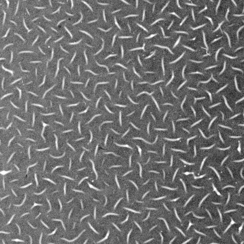
Figure 13: “Worms” in USNO-B. We found these unusual artifacts by looking at one of the places where our system failed to recognize SDSS images. The image is of the photographic plate POSS-IE 275, centered on $(\mathrm{RA},\mathrm{Dec})=(243,36)~{}\mathrm{degrees}$ and $15\times 15~{}\mathrm{arcmin}$ in size. Image credit: Copyright Palomar Observatory, National Geographic Society, and California Institute of Technology; courtesy of USNO Image and Catalogue Archive.

In order to determine the extent to which our failure to recognize images is due to problems with the USNO-B reference catalog, we built an index from the Two-Micron All-Sky Survey (2MASS) catalog, using the same process as for the USNO-B index, using the 2MASS $J$-band rather than the USNO-B red bands. We then asked our system to recognize each of the SDSS images that were unrecognized using the USNO-B-based index. Of the $61$ images, $51$ were recognized correctly, leaving only $10$ images unrecognized. Examining these images, we found that some contained bright, saturated stars which had been flagged as unreliable by the SDSS image-reduction pipeline. We retrieved the original data frames and asked our system to recognize them. All $10$ were recognized correctly: our source extraction procedure was able to localize the bright stars correctly, and with these the indexing system found a correct hypothesis. With these three processing steps, we achieve an overall performance of $100~{}\!\%$ correct recognition of all $182,221$ excellent images, with no false positives. This took a total of about $80$ minutes of CPU time. The index is about $5$ gigabytes in size, and once it is loaded into memory, multiple CPU cores can use it in parallel, so the wall-clock time can be a fraction of the total CPU time. During this experiment, a total of over $180$ million quads were tried, resulting in about $77$ million matches to quads in the index. Many of these matches were found to result in image scales that were outside the range we provided to the system, so the verification procedure was run only $6$ million times.

For completeness, we also checked the images that were rated as excellent but failed our selection cut. We retrieved the original images and used our source extraction routine and both the USNO-B- and 2MASS-based indexes. Our system was able to recognize correctly all $1138$ such images.

3.1.2 Performance on images of varying bandpass

In order to investigate the performance of our system when the bandpass of the query image is different than that of the index, we asked the system to recognize images taken through the SDSS filters $u$, $g$, $r$, $i$, and $z$. We used only the images rated “excellent”.

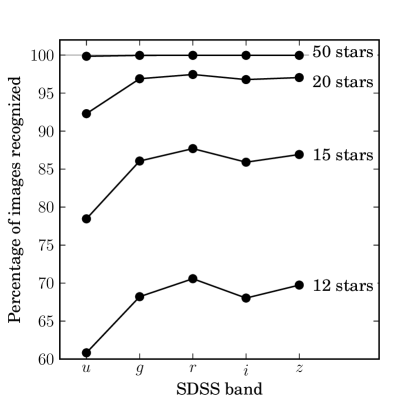
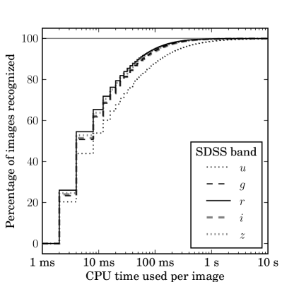
Figure 14: Performance on images taken through different SDSS bandpass filters. Left: The percentage of images recognized after building quads from a given number of the brightest stars in each image. The $r$-band is the best match to the USNO-B-based index we are using. Generally the recognition rate drops with the distance between the bandpass of the index and the bandpass of the image. The $i$-band performance in this instance is lower than expected. Right: The percentage of images recognized as the amount of CPU time spent per image increases. The $r$-band images are most quickly recognized, $g$-, $i$-, and $z$-band images take slightly more effort, and $u$-band images take considerably more CPU time. The asymptotic recognition rates are nearly identical except for $u$-band, which is slightly lower.

	Percentage of images recognized
CPU time	$u$	$g$	$r$	$i$	$z$
$0.1$ s	$87.80$	$93.88$	$94.87$	$93.59$	$94.36$
$1$ s	$98.58$	$99.73$	$99.78$	$99.73$	$99.75$
$10$ s	$99.82$	$99.96$	$99.97$	$99.96$	$99.96$
Final	$99.84$	$99.96$	$99.97$	$99.96$	$99.96$

The results, shown in the table above and in LABEL:~14, demonstrate that as the difference between the query image bandpass and the index bandpass increases, the amount of CPU time required to recognize the same fraction of images increases. This performance drop is more pronounced on the blue ($u$) side than the red ($z$) side. After looking at the brightest $50$ stars, the system is able to recognize essentially the same fraction of images. As shown by the first experiment in this section, this asymptotic recognition rate is largely due to defects in the reference catalog from which the index is built.

3.1.3 Performance on images of varying quality

In order to characterize the performance of the system as image quality degrades, we asked the system to recognize $r$-band images that were classified as “excellent”, “good”, “acceptable”, or “bad” by the SDSS image-reduction pipeline.

	Percentage of images recognized
CPU time	Excellent	Good	Acceptable	Bad
$0.1$ s	$94.87$	$94.85$	$94.57$	$84.11$
$1$ s	$99.78$	$99.74$	$99.64$	$96.58$
$10$ s	$99.97$	$99.94$	$99.94$	$99.11$
Final	$99.97$	$99.94$	$99.95$	$99.18$

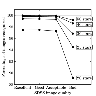
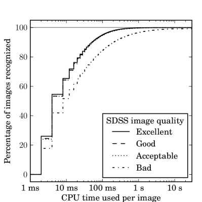
Figure 15: Performance of the system given images of varying quality. Left: The percentage of images recognized after looking at a given number of stars in each image, for excellent-, good-, acceptable-, and bad-quality images from SDSS. There is a small drop in performance for good and acceptable images, and a more significant drop for bad ones; all but the bad reach approximately the same asymptotic recognition rate. Right: CPU time per image for each quality rating. All but the bad images show nearly indistinguishable performance.

The results, shown in the table above and in LABEL:~15, show almost no difference in performance between excellent, good, and acceptable images. Bad images show a significant drop in performance, though we are still able to recognize over $99~{}\!\%$ of them.

3.1.4 Performance on images of varying angular size

We investigated the performance of our system with respect to the angular size of the images by cropping out all but the central region of the excellent-quality $r$-band images and running our system on the sub-images. Recall that the original image size is $13\times 9~{}\textrm{arcmin}^{2}$, and that the index we are using contains quads with diameters between $4$ and $5.6~{}\textrm{arcmin}^{2}$. We cut the SDSS images down to sizes $9\times 9$, $8\times 8$, $7\times 7$, and $6\times 6~{}\textrm{arcmin}^{2}$. The $7\times 7$ and $6\times 6$ images required much more CPU time, so we ran only small random subsamples of the images of these sizes.

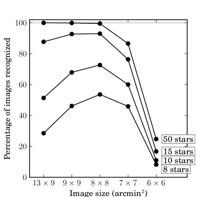
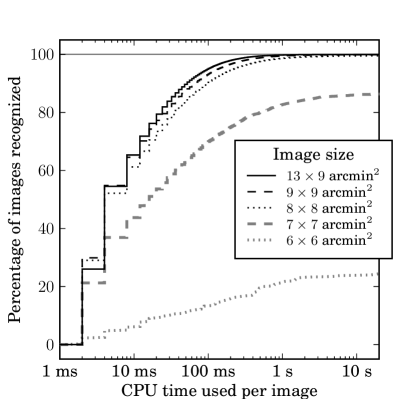
Figure 16: Performance of the system given images of varying angular sizes. Left: The percentage of images recognized after looking at a given number of stars in each image, for images of the given sizes. Perhaps surprisingly, more of the $8\times 8$ images are recognized correctly during the first few milliseconds, but as more time elapses, the larger-scale images are more likely to be recognized. Right: CPU time per image required to recognize images of each angular size. After $10~{}\mathrm{ms}$, the larger images are recognized more quickly. The $7\times 7$ and $6\times 6$ images appear to be reaching asymptotic recognition rates far below $100~{}\!\%$.

Image size (arcmin2)	Percentage of images recognized
$13\times 9$	$99.97$
$9\times 9$	$99.88$
$8\times 8$	$99.52$
$7\times 7$	$86.53$
$6\times 6$	$24.75$

The results, presented in the table above and in LABEL:~16, show that performance degrades slowly for images down to $8\times 8~{}\textrm{arcmin}^{2}$, and then degrades sharply. This is not surprising given the size of quads in the index used in this experiment: in the smaller images, only stars near the edges of the image can possibly be $4$ to $5.6~{}\mathrm{arcmin}$ away from another star, so the set of stars that can form the ‘backbone’ of a quad is small. Observe that images below $2.8\times 2.8~{}\textrm{arcmin}^{2}$ cannot possibly be recognized by this index, since no pair of stars can be $4~{}\mathrm{arcmin}$ or more away from each other.

This does not imply that small images cannot be recognized by our system: given an index containing smaller quads, we may still be able to recognize them. The point is simply that for any given index there is some threshold of angular size below which the image recognition rate will drop, and another threshold below which the recognition rate will be exactly zero.

3.1.5 Performance with varying image scale hints

In all the experiments above, we told our system the angular scale (in arcseconds per pixel) to within $\pm 1.25~{}\!\%$ of the true value, and we used an index containing only quads within a small range of diameters. In this experiment, we show that these hints merely make the recognition process faster without affecting the general results.

We created a set of sub-indices, each covering a range of $\sqrt{2}$ in quad diameters. The smallest-scale sub-index contains quads of $2$ to $2.8~{}\mathrm{arcmin}$, and the largest contains quads of about $20$ to $30$ degrees in diameter. Each sub-index is built using the same methodology as outlined above for the $4$ to $5.6~{}\mathrm{arcmin}$ index, with the scale adjusted appropriately. The smallest-scale sub-index contains only $6$ stars per HEALPix grid cell rather than $10$ as in the other sub-indices, because the USNO-B catalog does not contain enough stars: a large fraction of the smallest cells contain fewer than $10$ stars. In the smallest-scale sub-index we then do $9$ rounds of quad-building, reusing each star at most $5$ times, as opposed to $16$ rounds reusing each star at most $8$ times as in the rest of the sub-indices.

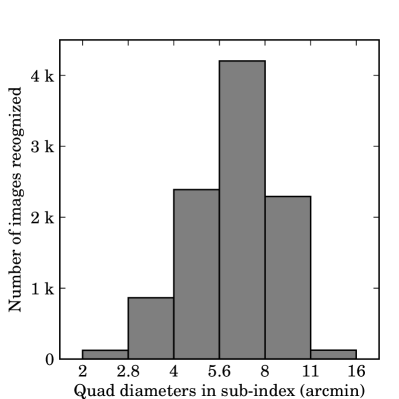
Figure 17: The sub-index that is first to recognize SDSS images, when all the sub-indices are run in lock-step. Although we used sub-indices containing quads up to $30$ degrees in diameter, clearly only the ones that contain quads that can possibly be found in an SDSS image (which are about $16~{}\mathrm{arcmin}$ across the diagonal) can generate correct hypotheses that will recognize the image. Perhaps surprisingly, each of these sub-indices is first to recognize some subset of the images, though a strong tuning effect is clear.

Each time our system examines a quad in the image, it searches each sub-index in turn for matching quads, and evaluates each hypothesized alignment generated by this process. The system proceeds in lock-step, testing each quad in the image against each sub-index in turn. The first quad match that generates an acceptably good alignment is taken as the result and the process stops. Note that several of the sub-indices may be able to recognize any given image. Indeed, LABEL:~17 shows that every sub-index that contains quads that can possibly be found in SDSS images is first to recognize some of the images in this experiment. Different strategies for ordering the computation—for example, spending equal amounts of CPU time in each sub-index rather than proceeding in lock-step—might result in better overall performance.

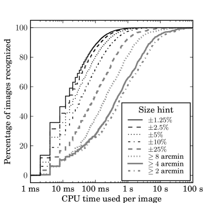
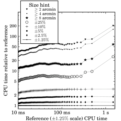
Figure 18: Performance of the system given varying limits on the image size. Left: CPU time per image required to recognize images, given various limits on the angular size of the image. Our system achieves the same asymptotic recognition rate in each case: giving the system less information about the true scale of the image simply means that it must evaluate and reject more false hypotheses before finding a true one. The “$\geq 8~{}\mathrm{arcmin}$” hint indicates that we told the system that the image width is between $8~{}\mathrm{arcmin}$ and $180~{}\mathrm{degrees}$. The upper limit has much less impact on performance than the lower limit, since the sub-indices that cover large angular scales contain many fewer quads and are therefore much faster to search, and generate fewer coincidental matches. Right: CPU time per image relative to the $\pm 1.25~{}\!\%$ case. We divided the CPU times for each case into percentiles; the mean time within each percentile is plotted. Generally, giving the system less information about the size of the images results in an approximately constant-factor increase in the CPU time required. Although there appears to be a sharp upward trend for the “loosest” four size ranges, this may be an effect of small sample size: since these cases take so long to run, we tested only $1000$ images, while for the rest of the cases we tested $10,000$ images. The CPU time distribution is heavy-tailed, so the expected variance is large.

3.1.6 Performance with varying index quad density

The fiducial index we have been using in these experiments contains about $16$ quads per HEALPix grid cell. Since each SDSS image has an area of about $7$ cells, we expect each image to contain about $100$ quad centers. The number of complete quads (i.e., quads for which all four stars are contained in the image) in the image will be smaller, but we still expect each image to contain many quads. This gives us many chances of finding a correct match to a quad in the image. This redundancy comes at a cost: the total number of quads in the index determines the rate of false matches—since the code-space volume is fixed, packing more quads into the space results in a larger number of matches to any given query point—which directly affects the speed of each query. By building indices with fewer quads, we can reduce the redundancy but increase the speed of each query. This does not necessarily increase the overall speed, however: an index containing fewer quads may require more quads from the image to be checked before a correct match is found. In this experiment, we vary the quad density and measure the overall performance.

	Percentage of images recognized
CPU time	$16$ quads/cell	$9$ quads/cell	$4$ quads/cell	$3$ quads/cell	$2$ quads/cell
$0.1$ s	$94.44$	$96.32$	$95.89$	$94.30$	$90.94$
$1$ s	$99.76$	$99.84$	$99.61$	$99.36$	$97.35$
$10$ s	$99.96$	$99.95$	$99.79$	$99.65$	$97.92$

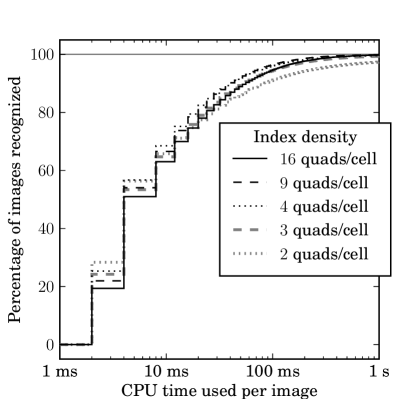
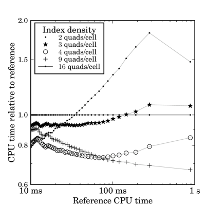
Figure 19: Performance of the system using indices containing varying densities of quads. (The total number of quads in an index is proportional to the density of quads.) Left: CPU time per image required to recognize images. Right: Relative CPU time to recognize images. We split the set of images into percentiles and have plotted the mean time within each percentile, relative to the 16-quad-per-cell reference index. The indices containing fewer quads are faster to search per quad query, but may require more quads to be tried before a correct match is found. The smaller indices are also able to recognize fewer images, because some images will simply not contain a quad that appears in the index. For the high-quality SDSS images we are using, the smallest of the indices here results in a $2~{}\!\%$ drop in recognition rate (from nearly $100~{}\!\%$ to about $98~{}\!\%$), but for poorer-quality images the drop could be larger.

As shown in the table above and LABEL:~19, reducing the density from $16$ to $9$ quads per HEALPix grid cell has almost no effect on the recognition rate but takes only two-thirds as much CPU time. Reducing the density further begins to have a significant effect on the recognition rate, and actually takes more CPU time overall.

3.1.7 Performance on indices built from triangles and quints

We tested the performance of our quad-based index against a triangle-based index and a quintuple-based (“quint”) index. The index-building processes were exactly as in our quad-based indices.

In the experiments above we searched for all matches within a distance of $0.01$ in the quad feature space. Since the triangle- and quint-based indices have feature spaces of different dimensionalities ($2$ for triangles, $6$ for quints), we first ran our system with the matching tolerance set to $0.02$ in order to measure the distribution of distances of correct matches in the three feature spaces. We then set the matching tolerance to include $95~{}\!\%$ of each distribution. For the triangle-based index, we found this matching tolerance to be $0.0064$, for the quad-based index it was $0.0095$, and for the quint-based index, $0.011$. These experiments were performed on a random subset of $4000$ images, because they are quite time-consuming.

	Percentage of images recognized
CPU time	Triangles	Quads	Quints
$0.1$ s	$0.20$	$57.45$	$23.35$
$1$ s	$28.07$	$92.20$	$36.67$
$10$ s	$78.58$	$99.28$	$72.75$
Final	$99.97$	$99.33$	$96.25$

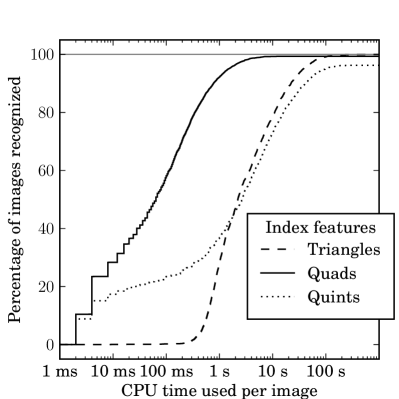
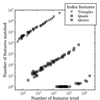
Figure 20: Performance of the system using indices containing triangles, quads, and quintuples of stars. Left: CPU time per image required to recognize images. The quad-based index vastly outperforms the triangle- and quint-based indices. Right: The number of features tried (i.e., the number of triangles, quads, or quints of stars from the image that were tested), and the number of matches to features in the index that resulted. Each plotted point summarizes $2~{}\!\%$ of the correctly-recognized images, sorted by the number of features tried. As expected, the triangle-based index produces many more matches for any given query, because the same number of features are packed into a lower-dimensional feature space. Fewer features have to be tried before the first correct matches are found, because only three corresponding stars have to be found. Quints, on the other hand, are very distinctive: for over $80~{}\!\%$ of the images that were correctly recognized, the first matching quint ever found was a correct match. However, many quints from the image have to be tested before this match is found.

The results are given in the table above and in LABEL:~20. After looking at the brightest $50$ stars in each image, the triangle-based index is able to recognize the largest number of images, but both the triangle- and quint-based indices take significantly more time than the quad-based index. It seems that quad features strike the right balance between being distinctive enough that any given query does not generate too many coincidental (false) matches—as the triangle-based index does—but containing few enough stars that it does not take long to find a feature that is in both the image and the index—as the quint-based index does.

We expect that the relative performance of triangle-, quad-, and quint-based indices depends strongly on the angular size of the images to be recognized. An index designed to recognize images of large angular size requires fewer features, so the code space is less densely filled and fewer false matches are generated. For this reason, we expect that above some angular size, a triangle-based index will recognize images more quickly than a quad-based index.

3.2 Blind astrometric calibration of Galaxy Evolution Explorer data

To show the performance of our system on significantly larger images, at a bandpass quite far from that of our index, we experimented with data from the Galaxy Evolution Explorer (GALEX). GALEX is a space telescope that observes the sky through near- and far-ultraviolet bandpass filters. Although it is fundamentally a photon-counting device, the GALEX processing pipeline renders images (by collapsing the time dimension and histogramming the photon positions), and these are the data products used by most researchers. The images are circular, with a diameter of about $1.2$ degrees. See LABEL:~21. In this experiment, rather than using the images themselves, we use the catalogs (lists of sources found in each image) that are released along with the images. These catalogs are produced by running a standard source extraction program (SExtractor) on the images. We retrieved the near-UV catalogs for all $28,182$ images in Galex Release 4/5 that have near-UV exposure.

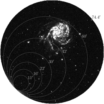
Figure 21: A sample GALEX field (AIS-101-sg32-nuv), with circles showing the sizes of the quads in the indices we use in this experiment. The images produced by the GALEX pipeline are $3840\times 3840$ pixels, and the near-UV field of view is a circle of diameter $1.24~{}\mathrm{degrees}$, or about $74.4~{}\mathrm{arcmin}$. Image credit: Courtesy NASA/JPL-Caltech.

We built a series of indices of various scales, each spanning roughly $\sqrt{2}$ in scale. The smallest contained quads with diameters from $11$ to $16~{}\mathrm{arcmin}$, the next contained quads between $16$ and $22~{}\mathrm{arcmin}$, followed by $22$ to $30$, $30$ to $42$, and $42$ to $60~{}\mathrm{arcmin}$. Each index was built according to the “standard recipe” given above, using stars from the red bands of USNO-B as before. In total these indices contain about $30$ million stars and $36$ million quads.

CPU time	Percentage of images recognized
1 s	74.46
10 s	93.56
100 s	98.95
Final	99.74

In this experiment, we told our system that the images were between $1$ and $2$ degrees wide, and we allowed it to build quads from the first $100$ sources in each image. The results are shown in the table above and LABEL:~22. The recognition rate is quite similar to that of the excellent-quality SDSS $r$-band fields, suggesting that even though the near-UV bandpass of these images is quite far from the bandpass of the index, which we would expect to make the system less successful at recognizing these images, their larger angular size seems to compensate. The system is significantly slower at recognizing GALEX images, but this is partly because we gave it a fairly wide range of angular scales, and because we used several indices rather than the single one whose scale is best tuned to these images.

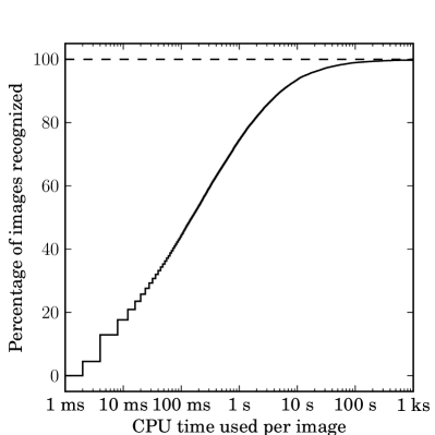
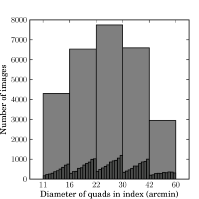
Figure 22: Results on GALEX near-UV images. Left: CPU time used per image. The shape of the curve is very similar to that in the previous SDSS experiments, though the “knee” of diminishing returns occurs after more CPU time (possibly because we gave the system much less information about the correct scale of the images). Right: The number of images recognized by each of the indices (identified by the range of sizes of quads they contain). For each quad in the image, we search for matches in each of the indices, stopping after the first match that is confirmed by the verification test. The histogram therefore shows only which index recognized the image first, rather than which indices might have recognized it given more time. The inset histograms show the distribution of quad sizes within each index (on a linear scale). Generally the larger quads are more successful, except in the largest index, where the size of the largest quads approaches that of the whole image.

3.3 Blind astrometric calibration of Hubble Space Telescope data

In order to demonstrate that there is nothing intrinsic in our method that limits us to images of a particular scale, we retrieved a set of Hubble Space Telescope (HST) images and built a custom index to recognize them. We chose the All-wavelength Extended Groth strip International Survey (AEGIS; Davis et al. 2007) footprint because it has many HST exposures and is within the SDSS footprint.

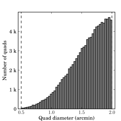
Figure 23: The diameters of quads in our custom index, built from SDSS stars, for recognizing Hubble Space Telescope Advanced Camera for Surveys (ACS) images in the AEGIS footprint. Although we allowed quads with diameters between $0.5$ and $2~{}\mathrm{arcmin}$, the size distribution of the quads that were created is heavily biased toward the large end of the range, because the density of SDSS stars—about $4$ per square arcminute—is not high enough to build many tiny quads.

To build the custom index for this experiment, we retrieved stars and galaxies from SDSS within a $2\times 2~{}\mathrm{degree}$ square centered on $\mathrm{RA}=215~{}\mathrm{degree}$, $\mathrm{Dec}=52.7~{}\mathrm{degree}$ with measured $r$-band brightness between $15$ and $22.2~{}\mathrm{mag}$, yielding about $57,000$ sources. We created the index as usual, using a HEALPix grid with cells of size $0.5~{}\mathrm{arcmin}$, and building quads with diameters between $0.5$ and $2~{}\mathrm{arcmin}$. This yielded just over $100,000$ quads. Since the density of stars and galaxies in our index is only about $4$ sources per square arcminute, the system tended to produce quads with sizes strongly skewed toward the larger end of the allowed range of scales. See LABEL:~23.

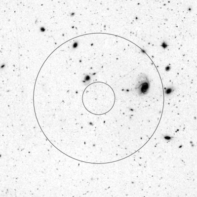
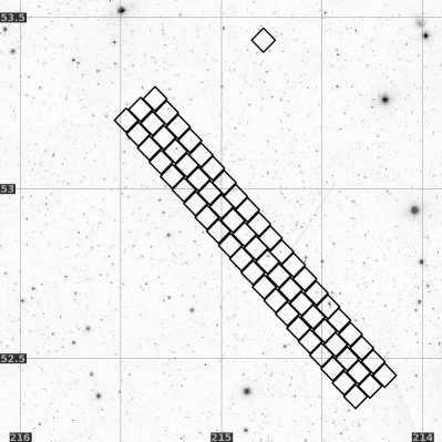
Figure 24: Left: A typical cutout of a Hubble Space Telescope Advanced Camera for Surveys (ACS) image as used in our experiment. The overlaid circles show the range of diameters of the quads in the index we use to recognize these images. ACS images are about $3.4~{}\mathrm{arcmin}$ square and $4096\times 4096$ pixels, but the cutouts we use in our experiment are about $3~{}\mathrm{arcmin}$ and have been downsampled to $600\times 600$ pixels. The quad diameters are from $0.5$ to $2~{}\mathrm{arcmin}$. Image credit: Courtesy NASA/JPL-Caltech. Right: A $\sim 2$ square degree region (part of the $\sim 4$ square degree region of SDSS from which we built our index), overlaid with the footprints of the $191$ ACS images that were recognized by our system. There are only $64$ unique footprint regions because some of the $191$ images are observations of the same region through different bandpass filters. The grid lines show $\mathrm{RA}$ and $\mathrm{Dec}$.

We queried the Hubble Legacy Archive (Jenkner et al., 2006) for images taken by the Hubble Advanced Camera for Surveys (ACS; Ford et al. 1998) within the AEGIS footprint. Since individual ACS exposures contain many cosmic rays, we requested only “level 2” images, which are created from multiple exposures and have cosmic rays removed. A total of $191$ such images were found. We retrieved $600\times 600$-pixel JPEG previews—see LABEL:~24 for an example—and gave these images to our system as inputs.

Our system successfully recognized $100~{}\!\%$ of the $191$ input images, taking an average of $0.3$ seconds of CPU time per image (not including the time required to perform source extraction). The footprints of the input images are shown in LABEL:~24. Although there are $191$ images, there are only $64$ unique footprints, because images were taken through several different bandpass filters for many of the footprints. Although the index contained quads with diameters from $0.5$ to $2~{}\mathrm{arcmin}$, the smallest quad that was used to recognize a field was about $0.9~{}\mathrm{arcmin}$ in diameter.

3.4 Blind astrometric calibration of other imagery

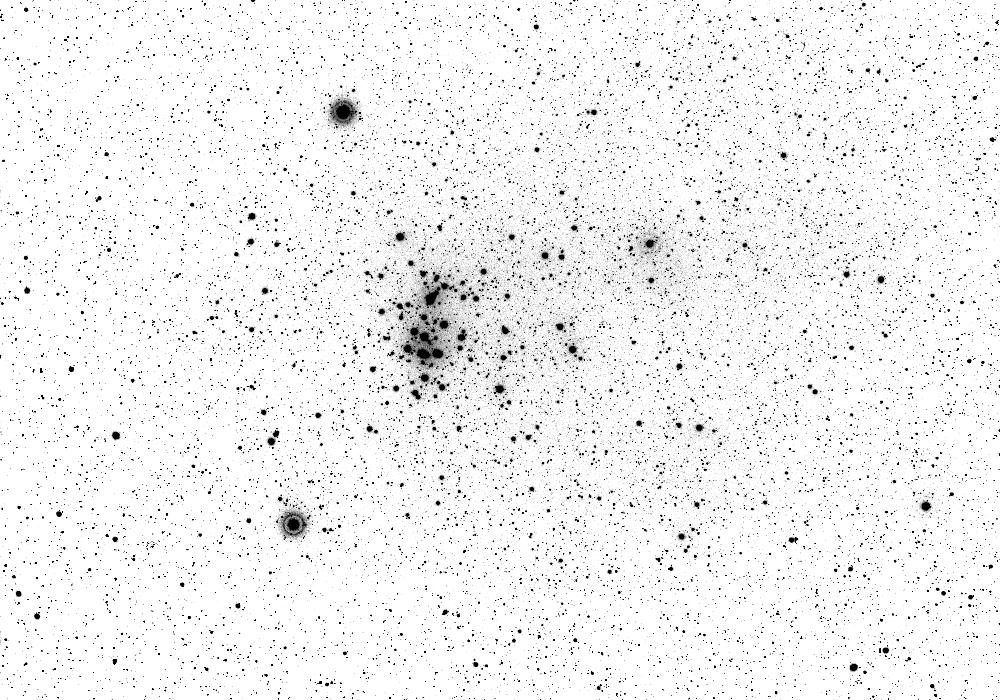
Figure 25: A sample DASCH scan of part of one of the photographic glass plates of the Harvard Observatory archives. The initial astrometric calibration of these plates is being computed by Astrometry.net. Praesepe, also known as the Beehive cluster or Messier 44, appears in this image. Image credit: DASCH team; Harvard College Observatory.

The Harvard Observatory archives contain over $500,000$ photographic glass plates exposed between 1880 and 1985. See LABEL:~25 for an example. The Digital Access to a Sky-Century at Harvard (DASCH) project is in the process of scanning these plates at high resolution (Mink et al., 2006; Grindlay et al., 2009). Since the original astrometric calibration for these plates consists of hand-written entries in log books, a blind astrometric calibration system was required to add calibration information to the digitized images. DASCH has been using the Astrometry.net system for the past year to create an initial astrometric calibration which is then refined by WCSTools (Mink, 2006).

The DeepSky project (Nugent et al., 2009) is reprocessing the data taken as part of the Palomar-QUEST sky survey and Nearby Supernova Factory (Djorgovski et al., 2009; Aldering et al., 2002). Since many of the images have incorrect astrometric meta-data, they are using Astrometry.net to do the astrometric calibration. Over $14$ million images have been successfully processed thus far (Peter Nugent, personal communication).

We have also had excellent success using the same system for blindly calibrating a wide class of other astronomical images, including amateur telescope shots, photographs from consumer digital SLR cameras, some of which span tens of $\mathrm{degrees}$. We have also calibrated videos posted to YouTube. These images have very different exposure properties, capture light in the optical, infrared and ultraviolet bands, and often have significant distortions away from the pure tangent-plane projection of an ideal camera. Part of the remarkable robustness of our algorithm, which allows it to calibrate all such images using the same parameter settings, comes from the fact that the hash function is scale invariant so that even if the center of an image and the edges have a significantly different pixel scale (solid angle per pixel), quads in both locations will match properly into the index (although our verification criterion may conservatively decide that a true solution with substantial distortion is not correct). Furthermore, no individual quad or star, either in the query or the index is essential to success. If we miss some evidence in one part of the image or the sky we have many more chances to find it elsewhere.

3.5 False positives

Although we set our operating thresholds to be very conservative in order to avoid false positive matches, images that do not conform to the assumptions in our model can yield false positive matches at much higher rates than predicted by our analysis. In particular, we have found that images containing linear features that result in lines of detected sources are often matched to linear flaws in the USNO-B reference catalog. We removed linear flaws resulting from diffraction spikes (Barron et al., 2008), but many other linear flaws remain. An example is shown in figures 26 and 27.

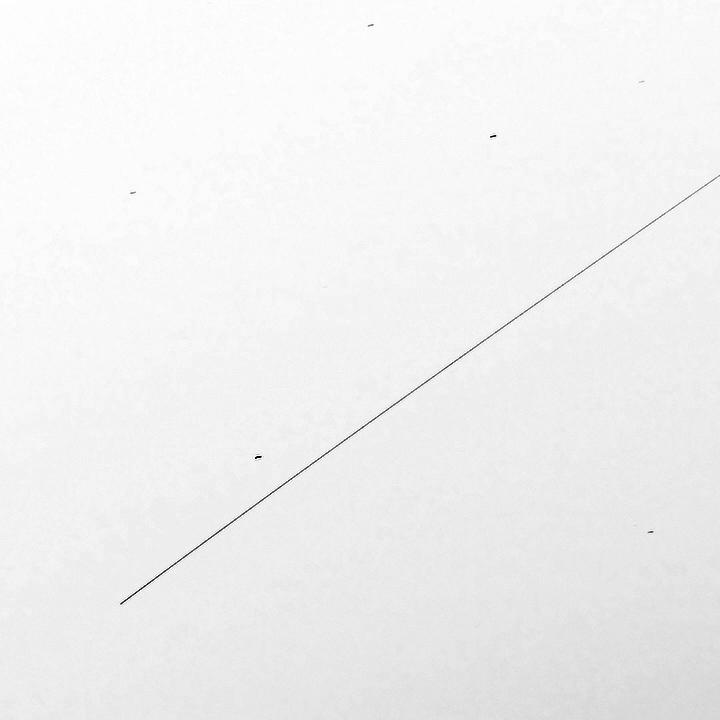
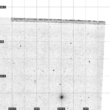
Figure 26: A false-positive match. Top: The input image contains a linear feature: the International Space Station streaked across the image. Image credit: copyright Massimo Matassi. Bottom: The USNO-B scanned photographic plate has writing on the corner. Image credit: copyright Palomar Observatory, National Geographic Society, and California Institute of Technology; courtesy of USNO Image and Catalogue Archive.

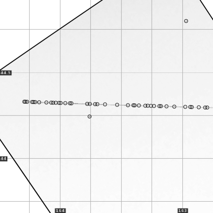
Figure 27: A false-positive match (continued). Top: The image, rotated to the alignment that our system found. The circles show the sources that were detected. The linear feature becomes a line of false sources. Bottom: The corresponding region of the USNO-B plate. The USNO-B source detection algorithm identifies many false sources in the region of text. The lines of sources in the two images are aligned in this (false) match.

4 Discussion

We have described a system that performs astrometric calibration—determination of imaging pointing, orientation, and plate scale—blind, or without any prior information beyond the data in the image pixels. This system works by using indexed asterisms to generate hypotheses, followed by quantitative verification of those hypotheses. The system makes it possible to vet or restore the astrometric calibration information for astronomical images of unknown provenance, and images for which the astrometric calibration is lost, unknown, or untrustworthy.

There are several sources of astronomical imagery that could be very useful to researchers—especially those studying the time domain—if they were consistently and correctly calibrated. These include photographic archives, amateur astronomers, and a significant fraction of professional imagery which has incorrect or no astrometric calibration meta-data. The photographic archives extend the time baseline up to a century, while amateur astronomers—some of whom are highly-skilled and well-equipped—can provide a dense sampling of the time domain and can dedicate a large amount of observing time to individual targets. Our system allows these sources of data to be made available to researchers by creating trustworthy astometric calibration meta-data.

The issue of trust is key to the success of efforts such as the Virtual Observatory to publish large, heterogeneous collections of data produced by many groups and individuals. Without trusted meta-data, data are useless for most purposes. Our system allows existing astrometric calibration meta-data to be verified, or new trustworthy meta-data to be created, from the data. Furthermore, applying a principled and consistent calibration procedure to heterogeneous collections of images enables the kinds of large-scale statistical studies that are made possible by the Virtual Observatory.

Our experiments on Sloan Digital Sky Survey, Galaxy Evolution Explorer, and Hubble Space Telescope images have demonstrated the capabilities and limitations of our system. The best performance, in terms of the fraction of images that are recognized and the computation effort required, is achieved when the index of known asterisms is well-matched to the images to be recognized. Differences in the bandpasses of the index and images lead to a small drop in performance across the near-infrared to near-ultraviolet range. By creating multiple indices across the spectrum we could overcome this limitation, if suitable reference catalogs were available. The image quality has some effect on the performance, though our experiments using the quality ratings assigned by the SDSS image-processing pipeline do not fully explore this space since the quality ratings are in terms of the very high standards of the survey: even the “bad” images are reasonable and over $99~{}\!\%$ of them can be recognized by our system. More experiments on images with poorly-localized sources would better characterize the behavior of the system on low-quality images.

In order to handle images across a wide range of scales, we build a series of indices, each of which is specialized to a narrow range of scales. Each index is able to recognize images within, and extending somewhat outside, the range to which it is tuned, but the drop-off in performance is quite fast: the index we used in the majority of our experiments works very well on $13\times 9~{}\mathrm{arcmin}^{2}$ SDSS images and sub-images down to $8\times 8~{}\mathrm{arcmin}^{2}$ but suffers a serious drop in performance on $7\times 7~{}\mathrm{arcmin}^{2}$ images. Similarly, the computational effort required is sharply reduced if the system is given hints about the scale of the images to be recognized. This is driven by three main factors. First, any index that contains quads that cannot possibly be found in an image of the given range of scales need not be examined. Second, only quad features of a given range of scales in the image need be tested. Finally, every quad in the image that is matched to a quad in the index implies an image scale, and any scale outside the allowed range can be rejected without running the verification procedure.

Using a set of indices, each of which is tuned to a range of scales, is related to the idea of co-visibility constraints in computer vision systems: “closely located objects are likely to be seen simultaneously more often than distant objects” (Yairi et al., 2001). Each of our indices contains the brightest stars within grid cells of a particular size, and contains quad features at a similar scale, so quads of large angular extent can only be built from bright stars, while small quads can be built from quite faint stars. This captures the practical fact that the angular scale of an image largely determines the brightnesses of the stars it contains. Distant pairs of faint stars are very unlikely to appear in the same image, and we take advantage of this constraint by only using faint stars to build quads of small angular size.

The index used in most of our experiments covers the sky in a dense blanket of quads. This means that in any image, we have many chances of finding a matching quad, even if some stars are missing from the image or index. This comes at the cost of increasing the number of features packed into our code feature space, and therefore the number of false matches that are found for any given quad in a test image. Reducing the number of quads means that each query will be faster, but more queries will typically be required before a match is found.

Our experiment using indices built from triangles and quintuples of stars shows that, for SDSS images, our geometric features built from quadruples of stars make a good tradeoff between being distinctive enough that the feature space is not packed too tightly, yet having few enough stars that the probability of finding all four stars in both the image and index is high. We expect that for images much larger in angular size than SDSS images, a triangle-based index might perform better, and for images smaller than SDSS images, a quint-based index might be superior.

Similarly, we found that using a voting scheme—requiring two or more hypotheses to agree before running the relatively expensive verification step—was slower than simply running the verification process on each hypothesis, when using a quad-based index and SDSS-sized images. In other domains (such as triangle-based indices), a voting scheme could be beneficial.

Although we have focused on the idea of a system that can recognize images of any scale from any part of the sky, our experiments on Hubble Space Telescope images demonstrate that by building a specialized index that covers only a tiny part of the sky, we can recognize tiny images that contain only a few stars that appear in even the deepest all-sky reference catalogs.

In principle, the geometric feature we are using requires that the images be conformal. That is, the images must be scaled, rotated versions of a tangent-plane project of the celestial sphere. Images with non-isotropic scaling (i.e., rectangular pixels) or shear in general cannot be recognized. It is possible to extend the system by using a different geometric feature that is invariant to these transformations; this requires adding at least one star to the set of stars used to define the local reference frame. In practice, we have found that although many images have some shear (indeed, the SDSS images that we have used as our primary test set have this property), the magnitude of the shear is typically small enough that it does not distort the geometric features very much. Even in images with significant shear or optical distortions, there are often regions of the image that are nearly conformal, and we are often able to recognize such images by finding a matching feature within a conformal region.

Our system, built on the idea of geometric hashing—generating promising hypotheses using a small number of stars and checking the hypotheses using all the stars—allows fast and robust recognition and astrometric calibration of a wide variety of astronomical images. The recognition rate is above $99.9~{}\!\%$ for high-quality images, with no false positives. Other researchers have begun using Astrometry.net to bring otherwise “hidden” data to light, and we hope to continue our mission “to help organize, annotate and make searchable all the world’s astronomical information.”

All of the code for the Astrometry.net system is available under an open-source license, and we are also operating a web service. See http://astrometry.net for details.

References

- Abazajian et al. (2009) Abazajian, K. N., et al. 2009, ApJS, 182, 543, arXiv:0812.0649
- Aldering et al. (2002) Aldering, G., et al. 2002, in Society of Photo-Optical Instrumentation Engineers (SPIE) Conference Series, ed. J. A. Tyson & S. Wolff, Vol. 4836, 61–72
- Barron et al. (2008) Barron, J. T., Stumm, C., Hogg, D. W., Lang, D., & Roweis, S. 2008, The Astronomical Journal, 135, 414
- Bertin (2005) Bertin, E. 2005, in Astronomical Data Analysis Software and Systems 15
- Bertin & Arnouts (1996) Bertin, E., & Arnouts, S. 1996, A&AS, 117, 393
- Davis et al. (2007) Davis, M., et al. 2007, ApJ, 660, L1, arXiv:astro-ph/0607355
- Djorgovski et al. (2009) Djorgovski, S. G., et al. 2009, in Bulletin of the American Astronomical Society, Vol. 41, Bulletin of the American Astronomical Society, 258–+
- Ford et al. (1998) Ford, H. C., et al. 1998, in Presented at the Society of Photo-Optical Instrumentation Engineers (SPIE) Conference, Vol. 3356, Society of Photo-Optical Instrumentation Engineers (SPIE) Conference Series, ed. P. Y. Bely & J. B. Breckinridge, 234–248
- Górski et al. (2002) Górski, K. M., Banday, A. J., Hivon, E., & Wandelt, B. D. 2002, in Astronomical Society of the Pacific Conference Series, Vol. 281, Astronomical Data Analysis Software and Systems XI, ed. D. A. Bohlender, D. Durand, & T. H. Handley, 107–+
- Grindlay et al. (2009) Grindlay, J., Tang, S., Simcoe, R., Laycock, S., Los, E., Mink, D., Doane, A., & Champine, D. 2009, Astronomical Society of the Pacific Conference Proceedings, in press
- Harvey (2004) Harvey, C. 2004, Master’s thesis, University of Toronto
- Huttenlocher & Ullman (1990) Huttenlocher, D. P., & Ullman, S. 1990, Int. J. Comput. Vision, 5, 195
- Ivezic et al. (2008) Ivezic, Z., Tyson, J. A., Allsman, R., Andrew, J., & Angel, R. 2008, LSST: from Science Drivers to Reference Design and Anticipated Data Products, arXiv:astro-ph/0805.2366
- Jenkner et al. (2006) Jenkner, H., Doxsey, R. E., Hanisch, R. J., Lubow, S. H., Miller, III, W. W., & White, R. L. 2006, in Astronomical Society of the Pacific Conference Series, Vol. 351, Astronomical Data Analysis Software and Systems XV, ed. C. Gabriel, C. Arviset, D. Ponz, & S. Enrique, 406–+
- Junkins et al. (1977) Junkins, J. L., White, III, C. C., & Turner, J. D. 1977, Journal of the Astronautical Sciences, 25, 251
- Lamdan et al. (1990) Lamdan, Y., Schwartz, J. T., & Wolfson, H. J. 1990, IEEE Transactions on Robotics and Automation, 6, 578
- Lang (2009) Lang, D. 2009, PhD in Computer Science, University of Toronto, 10 King’s College Road, Toronto, Ontario M5S 3G4, Canada
- Liebe (1993) Liebe, C. C. 1993, IEEE Aerospace and Electronic Systems Magazine, 8, 31
- Lupton et al. (2001) Lupton, R., Gunn, J. E., Ivezić, Z., Knapp, G. R., & Kent, S. 2001, in Astronomical Society of the Pacific Conference Series, Vol. 238, Astronomical Data Analysis Software and Systems X, ed. F. R. Harnden, Jr., F. A. Primini, & H. E. Payne, 269–+
- Martin & GALEX Science Team (2003) Martin, C., & GALEX Science Team. 2003, in Bulletin of the American Astronomical Society, Vol. 35, Bulletin of the American Astronomical Society, 1363–+
- Mink et al. (2006) Mink, D., Doane, A., Simcoe, R., Los, E., & Grindlay, J. 2006, in Virtual Observatory: Plate Content Digitization, Archive Mining and Image Sequence Processing, ed. M. Tsvetkov, V. Golev, F. Murtagh, & R. Molina, 54–60
- Mink (2006) Mink, D. J. 2006, in Astronomical Society of the Pacific Conference Series, Vol. 15, Astronomical Data Analysis Software and Systems XV, ed. C. Gabriel, C. Arviset, D. Ponz, & S. E., 204–+
- Monet et al. (2003) Monet, D. G., et al. 2003, AJ, 125, 984
- Nugent et al. (2009) Nugent, P. E., Palomar Transient Factory, & DeepSky Project. 2009, in Bulletin of the American Astronomical Society, Vol. 41, Bulletin of the American Astronomical Society, 419–+
- Pál & Bakos (2006) Pál, A., & Bakos, G. Á. 2006, The Publications of the Astronomical Society of the Pacific, 118, 1474
- Schade (2005) Schade, D. 2005, in Astronomical Society of the Pacific Conference Series, Vol. 338, Astrometry in the Age of the Next Generation of Large Telescopes, ed. P. K. Seidelmann & A. K. B. Monet, 156–+
- Skrutskie et al. (2006) Skrutskie, M. F., et al. 2006, AJ, 131, 1163
- Szalay (2001) Szalay, A. S. 2001, in Astronomical Society of the Pacific Conference Series, Vol. 238, Astronomical Data Analysis Software and Systems X, ed. F. R. Harnden, Jr., F. A. Primini, & H. E. Payne, 3–+
- Tody & Plante (2009) Tody, D., & Plante, R. 2009, Simple Image Access Specification Version 1.0, http://ivoa.net/Documents/PR/DAL/PR-SIA-1.0-20090521.html
- Valdes et al. (1995) Valdes, F. G., Campusano, L. E., Velasquez, J. D., & Stetson, P. B. 1995, PASP, 107, 1119
- Williams et al. (1996) Williams, R. E., et al. 1996, AJ, 112, 1335, arXiv:astro-ph/9607174
- Wolfson & Rigoutsos (1997) Wolfson, H. J., & Rigoutsos, I. 1997, IEEE Computational Science and Engineering, 4, 10
- Yairi et al. (2001) Yairi, T., Hirama, K., & Hori, K. 2001, in Intelligent Robots and Systems, 2001. Proceedings. 2001 IEEE/RSJ International Conference on, Vol. 3, 1263–1268 vol.3
- York et al. (2000) York, D. G., et al. 2000, AJ, 120, 1579, arXiv:astro-ph/0006396