A Second Method to Photometrically Align Multi-Site Microlensing Light Curves: Source Color in Planetary Event MOA-2007-BLG-192

Abstract

At present, microlensing light curves from different telescopes and filters are photometrically aligned by fitting them to a common model. We present a second method based on photometry of common field stars. If two spectral responses are similar (or the color of the source is known) then this technique can resolve important ambiguities that frequently arise when predicting the future course of the event, and that occasionally persist even when the event is over. Or if the spectral responses are different, it can be used to derive the color of the source when that is unknown. We present the essential elements of this technique and apply it to the case of MOA-2007-BLG-192, an important planetary event for which the system may be a terrestrial planet orbiting a brown dwarf or very low mass star. The refined estimate of the source color that we derive here $V-I=2.36\pm 0.03$ will aid in making the estimate of the lens mass more precise.

1 Introduction

The technical question most frequently asked of microlensers is “How do you align different data sets”? The standard answer is that data are aligned via a common microlensing model. That is, there is a microlensing magnification model $A(t)$, and the fluxes observed at the $i$th observatory are fit to $F_{i}(t)=f_{s,i}A(t)+f_{b,i}$, where $f_{s,i}$ is the instrumental source flux for that observatory and $f_{b,i}$ is blended light that does not participate in the event. This approach is very powerful: it allows microlensers to work with uncalibrated data, in non-standard filters, and to use difference image analysis (DIA) photometry without worrying about the flux zero point (which is simply absorbed into $f_{b}$). These advantages are all very important because microlensing data must often be analyzed very quickly, even when they come from unexpected quarters.

Nevertheless, there are instances when an alternative alignment method would be helpful. As we outline below (and discuss more extensively in Section 5) the need for such an alternative method has been at least subconsciously apparent for several years. However, we were motivated to systematically develop it by the problem of measuring the source color for the interesting planetary event, MOA-2007-BLG-192.

When microlensing planet searches were first proposed (Liebes, 1964; Mao & Paczyński, 1991; Gould & Loeb, 1992), there was no expectation that the planet masses, distances, planet-star physical separations, or orbital motion would be determined on an individual basis. Rather, it was thought that the quantities that could be measured were the planet/star mass ratio, $q$, and the planet-star projected separation $d$ in units of the Einstein radius, $\theta_{\rm E}$. Physical information about the planets would be restricted to statistical statements made about the ensemble of detections.

In fact, of the 9 microlensing planets published to date, the masses, projected separations, and distances are measured for four (Bond et al., 2004; Bennett et al., 2006; Udalski et al., 2005; Dong et al., 2009a; Gaudi et al., 2008), and are at least partly constrained for the rest (Beaulieu et al., 2006; Gould et al., 2006; Bennett et al., 2008; Dong et al., 2009b; Janczak et al., 2010). The primary reason for this turnabout is that, in strong contrast to garden-variety microlensing events, planetary events usually give rise to measurable finite-source effects. These then permit determination of

$$\rho\equiv{\theta_{*}\over\theta_{\rm E}},$$ (1)

the ratio of the angular source size to the angular Einstein radius. If $\theta_{*}$ can be determined, then one can measure $\theta_{\rm E}$

$$\theta_{\rm E}=\kappa M\pi_{\rm rel},\qquad\kappa\equiv{4G\over c^{2}\,\rm AU}\sim 8.1\,{{\rm mas}\over M_{\odot}},$$ (2)

where $M$ is the lens (host star) mass and $\pi_{\rm rel}$ is the lens-source relative parallax. If one can then obtain a constraint on another combination of lens mass and distance, from measuring e.g., the so-called “microlens parallax” (Gould, 2000), the flux from the lens (Han, 2005; Bennett et al., 2007), or astrometric offsets (Bennett et al., 2006; Dong et al., 2009a), then one can solve for both $M$ and $\pi_{\rm rel}$, and so obtain the planet mass (since $q$ is usually well-measured), as well as the distance to the lens. (Since the source is almost certainly in the Galactic bulge, $\pi_{\rm rel}$ directly yields the lens distance.)  The lens distance, $D_{\rm L}$, then allows one to infer the projected separation $r_{\perp}=D_{\rm L}\theta_{\rm E}d$. Even if no other constraints are obtained, however, measurement of $\theta_{\rm E}$ still yields the product $M\pi_{\rm rel}=\theta_{\rm E}^{2}/\kappa$, which then provides statistical constraints on the properties of the lens that are far better than if $\theta_{\rm E}$ is not measured.

Hence, there is a high premium on measuring $\theta_{\rm E}$ during planetary microlensing events. The standard method for doing this is to measure the dereddened color $(V-I)_{0}$ and magnitude $I_{0}$ of the source during the event. The dereddened color gives the surface brightness (Kervella et al., 2004), and the dereddened flux then gives the angular source size (Yoo et al., 2004). In fact, to a good approximation, all one really needs is the instrumental magnitude (which is automatically returned by the light curve model) and the instrumental color (which can be determined even without a model, just assuming that one has near-simultaneous photometry in $V$ and $I$ at several different magnification levels. The source can then be placed on an instrumental color-magnitude diagram (CMD) and compared to the position of the red giant clump, whose dereddened color and magnitude are known fairly well. Since the source suffers nearly the same extinction as the clump, one can directly determine $(V-I)_{0}$ and $I_{0}$ from such a diagram.

And therefore, microlensing planet hunters always try to obtain $V$-band measurement while the source is significantly magnified, to supplement the routinely-obtained $I$-band data. In fact, they try to obtain $H$-band data as well, since a 3-band $VIH$ determination can yield an even more precise measurement of $\theta_{*}$ (Bennett et al., 2010; Gould et al., 2009). Nevertheless, for a variety of reasons, including bad weather as well as the general chaos that is an indelible part of chasing after high-magnification microlensing events, sometimes these data are not taken or are not of adequate quality.

In the case of MOA-2007-BLG-192, no $V$-band data were taken simply because the event was not recognized as being sensitive to planets until after peak, and was not recognized as containing a planet until it had returned to baseline. Bennett et al. (2008) were nevertheless able to make a rough estimate of the source color by measuring the source magnitude (as described above) and assuming that it is a main-sequence star in the Galactic bulge. While these assumptions are not unreasonable, they lead to fairly large errors, and could in principle fail catastrophically if the source happened, e.g., to be in the Sagittarius Dwarf galaxy. Hence it would certainly be better to have a measured color than an estimated one. This is particularly true because the planetary system detected in this event is quite interesting. The most favored model is for a brown-dwarf host with a few-Earth-mass planet. Substantial work will be required to obtain the necessary constraints to confirm or reject this model (Bennett et al., 2008), but a color measurement (and so a measurement of $\theta_{*}$) would certainly be a step in the right direction.

Here we present a general method of obtaining such post-facto color measurements and apply it to MOA-2007-BLG-192. We find that it is somewhat redder than originally estimated, but well within the previous (appropriately generous) error bar.

The method can potentially be applied to obtain colors of other interesting microlensed sources. Perhaps even more important, it can be inverted to align data sets during the early phases of microlensing events when the model is poorly constrained, thus enabling much better real-time predictions, which are crucial to organizing observations. In some infrequent but nonetheless important cases, the relative flux normalizations from different observatories remain different for different event models, even after the event is over. Finally, it can be applied to obtain “microlens parallaxes” by aligning space-based and ground-based photometry. The method we describe here can be used to untangle all these cases as well.

2 General Method

To measure the color of archival events, we take advantage of the fact the microlensing data are often taken in non-standard bands. For example, there are many amateur observers who, because their telescopes generally have small apertures, often obtain unfiltered data or use very broad filters (Udalski et al., 2005; Gould et al., 2006, 2009; Gaudi et al., 2008; Janczak et al., 2010; Batista et al., 2009; Yee et al., 2009). And, very importantly for the present case, the MOA collaboration uses a broad $R/I$ filter, which we will refer to here as $R_{M}$. What one would like to do then, is to form an instrumental CMD by combining photometry of a common set of field stars in two bands, the first being a standard (or near-standard) $I$ band that is commonly used in microlensing studies and the second being a non-standard band. The source fluxes are (as mentioned in Section 1) routinely returned by the model of the event, so the source position could be firmly located on this non-standard CMD. Then one could identify the red-giant clump and measure the offset of the source from the clump (just as one does today in instrumental $V/I$ CMDs). The remaining step would be to make a color-color diagram that could relate the offset so measured to the $V-I$ offset in standard Johnson-Cousins bands.

In fact, as we will show in Section 3, such an approach is not possible, or at least not optimal. We adopt a course that draws its inspiration from this approach but is more flexible in dealing with several practical problems.

In the outline below, we will refer to the near-standard band as $I_{O}$ and the non-standard band as $R_{M}$, but the reader should keep in mind that the method can be used with any two bands, whether standard or non-standard, provided only that they have significantly different spectral response functions. The method requires $3\times 2=6$ flux alignments or “calibrations”. [(1) Measurement of source flux in instrumental system. (2) Calibration of field-star photometry relative to standard $V/I$. (3) Alignment of source photometry and field-star photometry.] $\times$ [(a) $R_{M}$. (b) $I_{O}$]

Before describing how we apply this approach to MOA-2007-BLG-192, it is worth reviewing how the same steps are “taken care of” in the more usual case when $V$ and $I$ photometry is obtained during the event. For step (1), the flux time series in the two bands are fit to the microlensing model. In fact, even if there is no model, the color can be determined from a model-independent regression of $V$ flux on $I$ flux. This is often done, for example, while the event is in progress and there is not yet a suitable model. Next, almost nothing must be done for step (2), since the photometry is already in standard (or near-standard) bands. Finally, step (3) usually requires no action at all. If one uses DoPHOT photometry (Schechter et al., 1993) for both the field stars and the light curve, then these are automatically on the same system. Of course, it is common practice to model light curves that are reduced using difference imaging analysis (DIA), (Woźniak, 2000; Alard, 2000), which is generally superior to DoPHOT for tracing the subtle details of planetary light curves. However, DoPHOT is generally more than adequate for the much coarser task of measuring the source color. Hence, in brief summary, for all three steps, almost nothing needs to be done that would not be done anyway. And this is perhaps the reason that it was not previously recognized that source colors could be obtained by combining non-standard photometry.

3 Application to MOA-2007-BLG-192

3.1 Instrumental Source Fluxes: DIA

As we show below, $\Delta(R_{M}-I_{O})/\Delta(V-I)=0.265$. Therefore, any error in instrumental $(R_{M}-I_{O})$ color (and so any error in the individual source fluxes) will be multiplied by a factor $\sim 4$ when we infer the $(V-I)$ color. This implies that we must attain maximum precision, which means using DIA rather than DoPHOT. In principle this should not present any special problems since both OGLE and MOA data are already reduced using DIA. However, for reasons described in Section 3.2, this does require that we re-reduce the MOA data using software derived from Woźniak (2000) DIA rather than the Bond et al. (2001) version normally used by MOA. Figure 1 shows the regression of measured (instrumental) source fluxes for the original OGLE data and the re-reduced MOA data, with respect to the magnification $A$ of the published event model of Bennett et al. (2008).

The slopes of the lines are the instrumental source fluxes $f_{s}$ because the observed difference flux is $f_{\rm obs}=Af_{s}+f_{b}$. (Note that the flux zero-point of this relation, $f_{b}$, plays no role in the result. This is important because difference imaging imposes an arbitrary zero-point on the reported fluxes.)  Outliers are recursively removed (crosses) if they exceed Gaussian expectations, the errors of the remaining points (circles) are renormalized to make $\chi^{2}$/dof = 1. The imperceptibly small scatter implies that the $f_{s}$ are very well determined (assuming that the model is correct): $R_{s,M}=23.0258\pm 0.0022$ and $I_{s,O}=21.4827\pm 0.0050$. Of course, the model is not perfectly determined, so in practice the error in the source flux is much larger. However, changes in the model normally move the source fluxes in tandem, so their ratio (and hence the source color) does not depend strongly on the model. If we ignore all such model variation, we can combine the above measurements of $f_{s}$ to obtain $(R_{M}-I_{O})_{s}=-2.5*\log(f_{s,M}/f_{s,O})=1.5431\pm 0.0060$. To find the effect of model changes, we explore an ensemble of models (Bennett et al., 2008) that all fit the data with $\Delta\chi^{2}\sim$ a few, and find that the color dispersion [weighted by $\exp(-\chi^{2}/2)$] is only 0.0025 (despite the fact that the dispersion in source magnitudes is 0.045). Adding this error in quadrature, we obtain,

$$(R_{M}-I_{O})_{s}=-2.5*\log{f_{s,M}\over f_{s,O}}=1.5431\pm 0.0065.$$ (3)

3.2 Calibration of Field-Star Photometry

In this section, we align both MOA and OGLE-III photometry from the event, with OGLE-II photometry (Szymański, 2005; Udalski et al., 1997). The latter is calibrated, so in this sense we are “calibrating” these two data sets. However, that is not our primary objective. Rather, we are mainly using OGLE-II data to align these two data sets with each other, and hence our primary focus is to carry out the alignments with OGLE-II in as similar a manner as possible. The main difficulty is that the MOA pixels are about twice as large as OGLE pixels and the seeing is about 2.5 times larger. Hence, our principal concern is that DoPHOT photometry of MOA “stars” will, on average, include “extra flux” relative to the corresponding OGLE-II stars, while OGLE-III stars will not. This would introduce a systematic error in the field-star calibration that is not paralleled in the $f_{s}$ measurements (which are done on difference images) and so would corrupt the color measurement.

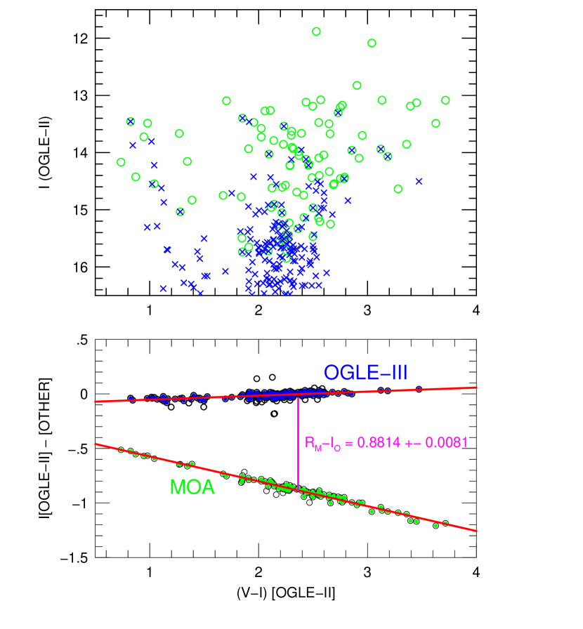
Figure 2: Lower panel: OGLE-III and MOA field stars are aligned with OGLE-II calibrated photometry. Only isolated stars are used for the comparison. Then $2.5\,\sigma$ outliers are recursively rejected (open circles) and remaining stars (filled circles) are fit to a straight line. The difference is $(R_{M}-I_{O})_{\rm fld}=+0.8646\pm 0.0025-(0.2648\pm 0.0044)[(V-I)-2.3]$ meaning that the MOA-OGLE spectral baseline has only 26.5% as much leverage as $V-I$. The vertical bar displays a geometric form of the final result. Its indicated height is just the sum of Eqs. (3) and (5). When it is moved to the left until it is wedged in the “jaws” of the MOA and OGLE color-color relations, its horizontal position gives the calibrated source color $(V-I)_{s}=2.363\pm 0.032$. Upper panel is a CMD of the accepted stars for MOA (circles) and OGLE-III (crosses).

To combat this difficulty we first construct a catalog of all astrometric matches within $0.12^{\prime\prime}$, without regard to magnitude offset. Next, we consider all stars in the OGLE-II catalog that lie within 3 FWHM of the matching catalog (whether MOA or OGLE-III). We compute the ratio of the brightness of the wing of this potentially contaminating star to the central brightness of the target star. If this ratio exceeds 1%, we exclude the target star from our sample. Next we consider all stars within 1 FWHM of the target and if any of these exceeds 2% of the total flux of the target, we also exclude the target. In this way, we ensure that the calibration is done only with isolated stars. Finally, we fit to a function of the form, $R_{M}=a+b(V-I)_{\rm OGLE-II}$, and recursively remove $2.5\,\sigma$ outliers. We also remove the handful of stars with $V-I>4$ because they are very far from our range of interest and have slightly larger scatter (although this hardly affects the calculation). The results for both MOA and OGLE-III are shown in Figure 2. Numerically, $I-R_{M,\rm fld}=-0.8696\pm 0.0021-(0.2280\pm 0.0035)[(V-I)-2.3]$, $I-I_{O,\rm fld}=-0.0050\pm 0.0013+(0.0368\pm 0.0027)[(V-I)-2.3]$, i.e.,

$$(R_{M}-I_{O})_{\rm fld}=+0.8646\pm 0.0025-(0.2648\pm 0.0044)[(V-I)-2.3].$$ (4)

3.3 Alignment of Field-Star and Light-Curve photometry

The MOA source flux was derived from the light curve in Section 3.1 using DIA photometry, while the field stars were calibrated in Section 3.2 using DoPHOT. These must still be put on the same system. In Woźniak (2000) DIA, the difference images are photometered using point-spread-function (PSF) fitting, and thus in principle the same procedure can be applied to the field stars in the frame, thus putting them on the same system. However, DIA PSF fitting is optimized in a very different way from DoPHOT PSF fitting. On the one hand, it must be able to measure negative fluxes (which DoPHOT cannot), and on the other hand it is dealing with difference images, which generally contain only variable stars and so are quite uncrowded. In particular, therefore, DIA PSF fitting makes no attempt to deblend stars. Thus, it can only be applied to isolated stars. Moreover, it appears to be less robust than DoPHOT in dealing with mildly non-linear to saturated pixels. Hence, to transform from the DIA-PSF to the DoPHOT system, one must make certain that comparison is made only on isolated stars and avoids stars with mildly non-linear pixels. We therefore begin by restricting our comparison sample to isolated stars as described in Section 3.2. These are shown in Figure 3. We exclude stars with $R<14.85$ because these have peak pixel values of 40,000 ADU, the point at which the CCD becomes mildly non-linear (Sako et al., 2004), and we exclude those with $R>16$ to avoid excessive scatter due to low signal. We find

$$(R_{M,\rm DoPHOT}-R_{M,\rm DIA})_{\rm fld}=-0.6617\pm 0.0049.$$ (5)

It appears visually from Figure 3 that our non-linearity threshold is sufficiently conservative, and we find that if we are yet more conservative and exclude stars with $R<15$, the result changes by $\ll 1\,\sigma$.

Note that the actual value of the offset $(-0.66)$ has no physical meaning. It is primarily the result of different normalization conventions used by DoPHOT and DIA. Secondarily, the DIA and DoPHOT templates are different, the former being constructed by stacking the best-seeing images, and the latter from an image in which the source is highly magnified (and so easily recognized by the DoPHOT software).

OGLE field stars are already on the DIA system, so no transformation is necessary, i.e., $I_{O,\rm fld}=I_{O,s}$. Hence, combining Equations (4) and (5) yields

$$(R_{M}-I_{O})_{s}=1.5263\pm 0.0055+(0.2648\pm 0.0044)[(V-I)-2.3],$$ (6)

which combined with Equation (3) yields

$$(V-I)_{s}=2.363\pm 0.032.$$ (7)

Figure 2 shows an alternative geometric derivation of this result. The height of the vertical bar is given by the sum of Equations (3) and (5). If it is moved to the left until it is wedged in the “jaws” comprising the MOA and OGLE color-color relations, its horizontal position gives the calibrated source color $(V-I)_{s}$.

4 Test of Method

We conduct a test of our method using a published event, MOA-2008-BLG-310 (Janczak et al., 2010) for which the source $(V-I)$ color can be determined from $V$ and $I$ light curves of the event. We stress that we work strictly in instrumental magnitudes, whereas Janczak et al. (2010) report results based on a calibrated version of the same data.

First, in analogy to Equation (3) we fit the instrumental MOA DIA and CTIO DoPHOT lightcurve fluxes to the magnifications found from the model to derive $(R_{\rm M,DIA}-I_{\rm CTIO})_{s}=0.6485\pm 0.0088$, where $R_{\rm M,DIA}$ is the instrumental MOA magnitude in the DIA system, and $I_{\rm CTIO}$ is the instrumental $I$-band magnitude in the CTIO DoPHOT system.

Next, we match uncrowded stars from the DoPHOT and DIA templates, and restrict consideration to the same flux range shown in Figure 3 to obtain $(R_{\rm M,\rm DoPHOT}-R_{\rm M,\rm DIA})_{\rm fld}=-0.9625\pm 0.0069$, in analogy to Equation (5). Adding these two equations yields $(R_{\rm M,DoPHOT}-I_{\rm CTIO})_{s}=-0.314\pm 0.011$.

Next, we use field stars to make an instrumental color-color plot of $(R_{\rm M,DoPHOT}-I_{\rm CTIO})$ vs. $(V-I)_{\rm CTIO}$ and find, in analogy to Equation (4), $(R_{\rm M,DoPHOT}-I_{\rm CTIO})_{\rm fld}=-0.3140\pm 0.0030+(0.155\pm 0.016)[(V-I)_{\rm CTIO}-0.3]$.

Finally, we combine the previous two equations to predict $(V-I)_{s,\rm CTIO,pred}=0.300\pm 0.071$. This can be compared with the instrumental color measured from the event light curve of $(V-I)_{s,\rm CTIO,meas}=0.310\pm 0.011$. This confirms, within the relatively large measurement error, that the method works.

Note that the prediction is less accurate in this case than for MOA-2007-BLG-192. This is mostly due to the shorter color baseline of $(R_{\rm MOA}-I_{\rm CTIO})$ relative to $(R_{\rm MOA}-I_{\rm OGLE-III})$. That is, CTIO $I$ is substantially bluer than OGLE-III $I$.

5 Discussion

5.1 Implications for MOA-2007-BLG-192

The color measurement presented here, $(V-I)_{s}=2.36\pm 0.03$, is 0.13 mag redder than, but within the (justifiably generous) error bar of $(V-I)_{s}=2.23\pm 0.20$ originally estimated by Bennett et al. (2008) based on the source apparent magnitude $I_{s}=21.45$ and the assumption that the source was a typical dwarf at the same distance as the observed clump stars. This redder color by itself implies a 20% lower surface brightness and so a 10% larger source radius, $\theta_{*}$. However, we also make several adjustments in the train of arguments that lead from $V/I$ measurements to $\theta_{*}$. We begin by adopting the Bennett et al. (2008) bulge clump color and absolute magnitude $[(V-I)_{0},M_{I}]_{\rm cl}=(1.04,-0.25)$ and clump distance modulus 14.38, as well as their logic leading to these values. Hence, $[(V-I),I]_{0,\rm cl}=(1.04,14.13)$. We remeasure the clump centroid on the CMD and find $[(V-I),I]_{\rm cl}=(2.16,15.65)$. Together, these imply $[(V-I),I]_{0,s}=[(V-I),I]_{s}-[(V-I),I]_{\rm cl}+[(V-I),I]_{0,\rm cl}=(1.24,19.93)$. Most importantly, we use the very tight $VIK$ color-color relations of Bessell & Brett (1988) to infer $[(V-K),K]_{0}=(2.81,18.36)$ and then use the very tight Kervella et al. (2004) $V/K$ surface-brightness relations to obtain $\theta_{*}=0.57\,\mu$as.

To estimate the new error bar, we first note that the error in the clump-offset method for estimating $(V-I)_{0}$ (Yoo et al., 2004) has been determined to be 0.05 mag by direct comparison with highly magnified dwarf stars using high-resolution spectra (J.A. Johnson, 2008 private communication). This implies $(V-I)_{0}=1.24\pm 0.06$, which by itself yields a fractional error in $\theta_{*}$ of 3%. There are additional errors of of 0.045 mag uncertainly in the model fit for the source flux, of 0.04 mag in centroiding the height of the clump, as well as much smaller errors in the Bessell & Brett (1988) and Kervella et al. (2004) relations. Thus $\theta_{*}=0.570\pm 0.025\,\mu$as. Finally, we state separately the error due to the assumed Galactocentric distance $R_{0}=8.0\pm 0.4$ kpc (since this may be resolved in the relatively near future) and finally find $\theta_{*}=0.57\pm 0.04\,\mu$as, compared to $\theta_{*}=0.50\pm 0.10\,\mu$as from Bennett et al. (2008). Hence, this color measurement essentially removes one of the important uncertainties in characterizing the planet.

A key future test for the brown-dwarf hypothesis would be to image the lens-source system using the adaptive optics on large telescopes or the Hubble Space Telescope, at various degrees of separation (Alcock et al., 2001; Kozlowski et al., 2007). Because of the expected faintness of the lens (regardless of the whether it is a brown dwarf or a late M dwarf), independent knowledge of the source color would be important in the interpretation of these images.

5.2 Application to Event Prediction

While we have presented our method in the context of measuring the source color given a reasonably well-determined model, it can easily be inverted to constrain models when traditional methods of flux alignment fail. The most common case is that microlensing survey groups often notify the community of newly discovered events and then go offline, either for short periods due to daylight or for longer periods due to weather. The events are then often monitored by other observers, but the observations generally cannot be aligned with the discovery data (with their long time baseline) using the traditional model-fitting technique because the models are completely degenerate. We have shown here that with good data, the source fluxes, $f_{s}$, for different data sets can be aligned to better than 1%, provided that the source color is known. As mentioned in Section 1, the color can be measured even without a model, and even if it not measured, the alignment can be done from color estimates provided that the spectral responses of the two instruments are sufficiently close. Of course, there will be uncertainties in these alignments, but compared to the present situation of complete ignorance, this would be a vast improvement and would lead to greatly improved predictions of future event behavior. This is especially important for high-magnification events, which are the most sensitive to planets, and which often are not discovered or not recognized to be high-magnification, until a few hours before peak. OGLE-2007-BLG-224 was an extreme example of this (Gould et al., 2009).

5.3 Application to Event Analysis

In some cases, different data sets cannot be aligned by the traditional technique, even after the event is over. For example, V. Batista (2007 private communication) found that MOA-2007-BLG-146 had two very different binary-lens solutions, that differed strongly in their relative flux normalizations for different observatories. Another example is the planetary event OGLE-2005-BLG-071. Dong et al. (2009a) reported that there were data over one of the peaks from MDM and Palomar that could have helped constrain the measurement of $\rho=\theta_{*}/\theta_{\rm E}$, but whose value was substantially degraded because they could not be normalized to other data sets. And there are several planetary events currently under analysis for which such flux degeneracies are a significant obstacle to resolving model degeneracies. The technique described here would be useful in all these cases.

5.4 Application to Space-Based Parallaxes

When Gould (1995) proposed obtaining microlens parallaxes using a single satellite, he argued that the spectral responses of the space-based and ground-based cameras should be the same, or at least that their differences should be known with extremely high precision ($\Delta\bar{\lambda}\lesssim 2\,$nm). This precision requirement is rooted in the basic physics of the measurement: microlens parallax is derived from the difference in magnifications as seen from two separated observers, but what is actually measured is the difference in fluxes. The observed flux is given by $f=f_{s}A+f_{b}$, so to derive $A$ from $f$, one must know $f_{s}$ and $f_{b}$, which depend on the overall microlensing model. One can remove part of this ambiguity (namely $f_{b}$) by subtracting a baseline image $(A=1)$ from a magnified image. Then one obtains $\Delta f=(A-1)f_{s}$. However, $f_{s}$ remains a fit parameter for both observatories, which can have several percent errors, particularly if (as expected) there are not many space-based measurements. However, Gould (1995) argued, that if the spectral responses were known to be the same, then even if the two $f_{s}$ were not measured with great precision, the ratio of their values would move in tandem, so that the magnification difference (needed for the parallax measurement) would be known much better than the absolute magnification. The method of light-curve alignment presented here can serve as a practical substitute for identical spectral responses (which would be extremely difficult given that one telescope is sitting below the Earth’s atmosphere).

6 Conclusions

We have presented a method for aligning microlensing light curves from different observatories that is independent of the standard method, which is based on fitting to a common model. We were initially motivated to develop this technique in order to measure the source color for the archival event MOA-2007-BLG-192, which is a candidate brown-dwarf lens hosting a terrestrial planet. We succeeded in measuring this color within $\sigma(V-I)=0.03$, which will aid in future efforts to characterize this planetary system.

We have argued that the same technique potentially has much broader uses, not only to find the colors of other source stars, but also in the timely recognition of high-magnification events and real-time analysis of anomalous events, which are both critical to the data-gathering stage of microlensing studies, as well as to the analysis of already-completed events. Finally, we have shown that the technique can be used derive otherwise unobtainable microlens parallaxes by aligning Earth-based and space-based lightcurves.

Figure 1: Regression of instrumental fluxes from OGLE and MOA against the published magnification model of Bennett et al. (2008). The slopes give the instrumental source fluxes $f_{s}$. Outliers beyond Gaussian expectation are recursively rejected (crosses). Remaining points (circles) have errors renormalized to $\chi^{2}$/dof = 1. The instrumental source fluxes $f_{s}$ are given by the slopes, and the instrumental color is $(R_{M}-I_{O})=-2.5*\log(f_{s,M}/f_{s,O})=1.5431\pm 0.0065$, where $R_{M}$ and $I_{O}$ are the instrumental MOA and OGLE-III passbands, respectively.

Figure 3: Offset between DoPHOT and DIA-PSF photometry for MOA data, the former being designed for (unchanging) field stars and the latter for difference images containing an (isolated) source. The DIA PSF can therefore only be applied to isolated field stars, which are shown here. Stars outside the dashed lines are too bright (and hence non-linear) or too faint (and hence have too low signal) to be included. Offset is $R_{M,\rm DoPHOT}-R_{M,\rm DIA}=-0.6617\pm 0.0049$.

References

- Alard (2000) Alard, C., 2000, A&AS, 144, 363
- Alcock et al. (2001) Alcock, C. et al. 2001, Nature, 414, 617
- Batista et al. (2009) Batista, V. et al. 2009, A&A, submitted, arXiv:0907.3471
- Beaulieu et al. (2006) Beaulieu, J.-P. et al. 2005, Nature, 439, 437
- Bessell & Brett (1988) Bessell, M. S., & Brett, J. M. 1988, PASP, 100, 1134
- Bennett et al. (2006) Bennett, D.P., Anderson, J., Bond, I. A., Udalski, A., & Gould, A. 2006, ApJ, 647, L171
- Bennett et al. (2007) Bennett, D.P., Anderson, J., & Gaudi, B.S. 2007, ApJ, 660, 781
- Bennett et al. (2008) Bennett, D.P. et al., 2008, ApJ, 684, 663
- Bennett et al. (2010) Bennett, D.P. et al., 2010, in preparation
- Bond et al. (2001) Bond, I.A., et al. 2001, MNRAS, 327, 868
- Bond et al. (2004) Bond, I.A., et al. 2004, ApJ, 606, L155
- Dong et al. (2009a) Dong, S., et al. 2009a, ApJ, 695, 442
- Dong et al. (2009b) Dong, S., et al. 2009b, ApJ, 698, 1826
- Gaudi et al. (2008) Gaudi, B. S., et al. 2008, Science, 319, 927
- Gould & Loeb (1992) Gould, A., & Loeb, A. 1992, ApJ, 396, 104
- Gould (1995) Gould, A., et al. 1995, ApJ, 441, L21
- Gould (2000) Gould, A., et al. 2000, ApJ, 542, 785
- Gould et al. (2006) Gould, A., et al. 2006, ApJ, 644, L37
- Gould et al. (2009) Gould, A., et al. 2009, ApJ, 698, L147
- Han (2005) Han, C. 2005, ApJ, 633, 414
- Janczak et al. (2010) Janczak, J. et al. 2010, ApJ, submitted arXiv:0908.0529
- Kervella et al. (2004) Kervella, P., Thévenin, F., Di Folco, E., & Ségransan, D. 2004, A&A, 426, 297
- Kozlowski et al. (2007) Kozlowski, S., Woźniak, P.R., Mao, S., & Wood, A. 2007, ApJ, 671, 420
- Liebes (1964) Liebes, S. 1964, Physical Review, 133, 835
- Mao & Paczyński (1991) Mao, S. & Paczyński, B. 1991, ApJ, 374, L37
- Sako et al. (2004) Sako, T., et al. 2004, arXiv:804.0653
- Schechter et al. (1993) Schechter, P.L., Mateo, M. & Saha, A. 1993, PASP, 105 1342
- Szymański (2005) Szymański, M.K. 2005, Acta Astronomica, 55, 43
- Udalski et al. (1997) Udalski, A., Kubiak, & Szymański, M.K. 1997, Acta Astronomica, 47, 319
- Udalski et al. (2005) Udalski, A., et al. 2005, ApJ, 628, L109
- Woźniak (2000) Woźniak, P.R. 2000, Acta Astron., 50, 421
- Yee et al. (2009) Yee, J.C. et al. 2009, ApJ, ApJ, 703, 2082
- Yoo et al. (2004) Yoo, J. et al. 2004, ApJ, 603, 139