Finite Connections for Supercritical Bernoulli Bond Percolation in 2D

Abstract.

Two vertices ${\sf x}$ and ${\sf y}$ are said to be finitely connected if they belong to the same cluster and this cluster is finite. We derive sharp asymptotics (1.2) of finite connections for super-critical Bernoulli bond percolation on ${\mathbb{Z}}^{2}$.

1. Introduction and Results

In the case of the two dimensional nearest neighbour Ising model below critical temperature, truncated two-point functions could be computed exactly,

$$g({\sf x})=\left\langle\sigma_{0};\sigma_{{\sf x}}\right\rangle^{\,}_{\beta}\,=\,\frac{\phi({\sf n}_{{\sf x}})}{\lvert{\sf x}\rvert^{2}}{\rm e}^{-2\tau_{\beta}({\sf x})}\left(1+o(1)\right),$$ (1.1)

where $\tau_{\beta}$ is the surface tension, ${\sf n}_{{\sf x}}={\sf x}/\lvert{\sf x}\rvert\in{\mathbb{S}}^{1}$ and $\phi$ is a positive locally analytic function on ${\mathbb{S}}^{1}$.

In this paper we rigorously derive a version of (1.1) for the simplest non exactly solvable two dimensional model: the super-critical Bernoulli bond percolation on two-dimensional square lattice. The model is self-dual: let $p^{*}>1/2$, and consider sub-critical Bernoulli bond percolation measure ${\mathbb{B}}_{p}$ on the direct lattice ${\mathbb{Z}}^{2}$ with $p=1-p^{*}$. Let $\mathcal{E}^{2}$ be the set of all nearest neighbour direct bonds. Each direct bond $b\in\mathcal{E}^{2}$ intersects exactly one dual bond $b_{*}\in\mathcal{E}^{2}_{*}$ of the dual lattice ${\mathbb{Z}}_{*}^{2}=(1/2,1/2)+{\mathbb{Z}}^{2}$. Thus each direct percolation configuration $\eta\in\left\{0,1\right\}^{\mathcal{E}^{2}}$ unambiguously corresponds to the dual configuration $\eta_{*}\in\left\{0,1\right\}^{\mathcal{E}^{2}_{*}}$ via

$$\eta(b)\,=\,1\quad\Longleftrightarrow\quad\eta_{*}(b_{*})\,=\,0.$$

Of course, the induced measure on $\left\{0,1\right\}^{\mathcal{E}^{2}_{*}}$ is just the super-critical Bernoulli bond percolation at $p^{*}$ and we shall causally take advantage of the fact that both models are defined on the same probability space and, furthermore, we shall use the same notation ${\mathbb{B}}_{p}$ for both.

Two dual lattice points ${\sf x}^{*},{\sf y}^{*}\in{\mathbb{Z}}^{2}$ are said to be finitely connected; $\{{\sf x}^{*}\stackrel{{\scriptstyle{\rm f}}}{{\longleftrightarrow}}{\sf y}^{*}\}$, if there exists a path of open dual bonds $\gamma^{*}$ leading from ${\sf x}^{*}$ to ${\sf y}^{*}$, but the cluster $\mathbf{Cl}({\sf x}^{*})$ of ${\sf x}^{*}$ (and hence the cluster $\mathbf{Cl}({\sf y}^{*})$) is finite. The truncated two-point function is defined then as

$$g({\sf x}^{*})={\mathbb{B}}_{p}\left(0^{*}\stackrel{{\scriptstyle{\rm f}}}{{\longleftrightarrow}}{\sf x}^{*}\right),$$

where $0^{*}\stackrel{{\scriptstyle\Delta}}{{=}}(1/2,1/2)$. For simplicity we shall consider only on-axis directions, that is we shall focus on asymptotics of $g({\sf x}_{N}^{*})$ for ${\sf x}_{N}^{*}\stackrel{{\scriptstyle\Delta}}{{=}}(N+1/2,1/2)$. It should be noted, however, that our approach goes through with only minor modifications for arbitrary lattice directions.

Theorem A.

For every $p^{*}=1-p>p_{c}=1/2$ there exists a constant $\psi=\psi(p^{*})>0$ such that

$$g({\sf x}_{N}^{*})\,=\,{\mathbb{B}}_{p}\left(0^{*}\stackrel{{\scriptstyle{\rm f}}}{{\longleftrightarrow}}{\sf x}_{N}^{*}\right)\,=\,\frac{\psi}{N^{2}}{\rm e}^{-2N\tau_{p}({\sf e}_{1})}\left(1+o(1)\right),$$ (1.2)

where ${\sf e}_{1}=(1,0)$ and $\tau_{p}(\cdot)$ is the inverse correlation length of the sub-critical model (equivalently, the surface tension of the dual super-critical model).

The logarithmic asymptotics ${\rm e}^{-2N\tau_{p}({\sf e}_{1})}$ can be established by relatively soft arguments [CCGKS]: roughly speaking the event $\left\{0^{*}\stackrel{{\scriptstyle{\rm f}}}{{\longleftrightarrow}}{\sf x}_{N}^{*}\right\}$ implies two disjoint sub-critical connections over the strip $\left\{(x,y):0\;\leqslant\;x\;\leqslant\;N\right\}$. The main struggle here is to recover asymptotics of finite connection probabilities up to zero order terms, the correct order $1/N^{2}$ of the prefactor in particular. This amounts to developing a detailed stochastic geometric characterization of long finite super-critical clusters, which may be considered as the principle new result of this paper.

Sharp asymptotitcs of finite connections for $d$-dimensional ($d\;\geqslant\;3$) high-density models were recently investigated in [BPS1, BPS2]. In the case of higher dimensions the order of the prefactor is $N^{-(d-1)/2}$. This is the classical off-critical Ornstein-Zernike prefactor. The expected non-Ornstein-Zernike order of prefactor $N^{-2}$ in (1.2) in two-dimensions was clearly understood and discussed on heuristic level in an earlier literature, see e.g. [BF, BPS2]: The conventional OZ picture comes from the fluctuation theory of one-dimensional systems. However, finite connections in two dimensions are described in terms of fluctuation theory of two interacting one dimensional effective random walk type structures.

Let us elaborate on the latter point. Both the direct sub-critical percolation model at $p<1/2$ and the dual super-critical model at $p^{*}=1-p>1/2$ are defined on the same probability space.

In particular, the event $\left\{0^{*}\stackrel{{\scriptstyle{\rm f}}}{{\longleftrightarrow}}{\sf x}_{N}^{*}\right\}$ can be written as (see Figure 1)

$$\left\{0^{*}\stackrel{{\scriptstyle{\rm f}}}{{\longleftrightarrow}}{\sf x}_{N}^{*}\right\}\,=\,\left\{0^{*}\longleftrightarrow{\sf x}_{N}^{*}\right\}\cap\mathcal{C}_{N},$$ (1.3)

where $\left\{0^{*}\longleftrightarrow{\sf x}_{N}^{*}\right\}$ means that $0^{*}$ and ${\sf x}_{N}^{*}$ are connected in the dual model and the event $\mathcal{C}_{N}$ is defined in terms of the direct percolation model via

$$\mathcal{C}_{N}\,=\ \,\Bigl{\{}\eta\in\left\{0,1\right\}^{\mathcal{E}^{2}}\,:\,\exists\,\,\text{an open direct loop around $0^{*}$ and ${\sf x}_{N}^{*}$}\Bigr{\}}.$$ (1.4)

Figure 1. The event $\left\{0^{*}\stackrel{{\scriptstyle{\rm f}}}{{\longleftrightarrow}}{\sf x}_{N}^{*}\right\}\,=\,\left\{0^{*}\longleftrightarrow{\sf x}_{N}^{*}\right\}\cap\mathcal{C}_{N}$: $\gamma^{*}:0^{*}\rightarrow{\sf x}_{N}^{*}$ is a dual (super-critical) open path, whereas $\mathfrak{C}_{N}$ is an open direct (sub-critical) loop-like cluster. The cluster $\mathfrak{C}_{N}$ splits into irreducible loops around $0^{*}$ and ${\sf x}_{N}^{*}$ and a pair of disjoint connections from ${\sf x}$ to ${\sf y}$ and from ${\sf v}$ to ${\sf u}$.

We shall use $\mathfrak{C}_{N}$ to denote the inner-most connected component which contains such a loop, and we shall decompose $\{0^{*}\stackrel{{\scriptstyle{\rm f}}}{{\longleftrightarrow}}{\sf x}_{N}^{*}\}$ according to geometric properties of $\mathfrak{C}_{N}$. We shall see that a typical $\mathfrak{C}_{N}$ can be split as it is schematically depicted on Figure 1: There are “irreducible” dual percolation loops from ${\sf v}$ to ${\sf x}$ around $0^{*}$ and, respectively, from ${\sf u}$ to ${\sf y}$ around ${\sf x}_{N}^{*}$. In the middle strip $\left\{(x,y):\ell\;\leqslant\;x\;\leqslant\;N-r\right\}$ there are disjoint connections from ${\sf v}$ to ${\sf u}$ and from ${\sf x}$ to ${\sf y}$. The notion of irreducibility will be set up in such a way that $\ell$ and $r$ will be typically small and will be eventually integrated out. The crux of the matter is to understand how to compute the probability of the double connection event in the middle strip. The main thrust of the theory developed in [CI, CIV1, CIV3] is that on large finite scales sub-critical percolation clusters have effective random walk structure. One of our two main results here is a reformulation of the double connection event in the middle strip in terms of hitting probabilities for two effective random walks conditioned on non-intersection. The second main result is an adjustment of the fluctuation identities introduced in [AD, BJD] for computing these probabilities.

Effective random walk picture

We proceed with a description of our effective random walk picture as it will show up in the reformulation of the double connection event. Let $\left\{\sigma_{k}=(\rho_{k},\xi^{1}_{k},\xi^{2}_{k})\right\}$ be a collection of i.i.d. ${\mathbb{N}}\times{\mathbb{Z}}^{2}$-valued random variables defined on some probability space equipped with a probability measure ${\mathbb{P}}$ and satisfy the following set of conditions:

(P1) There exists $\alpha<\infty$ such that

$${\rm Range}(\sigma)\,=\,\left\{(t,v,x)\,:\,\lvert v\rvert,\lvert x\rvert<\alpha t\right\}.$$

(P2) There exists $\beta>0$ such that (for the exact definition of “$\lesssim$” see the remark on notational convention below)

$${\mathbb{P}}\left(\rho>t\right)\,\lesssim\,{\rm e}^{-\beta t}.$$

(P3) For any $t\in{\mathbb{N}}$ the conditional (on $\rho=t$) distribution of $(\xi^{1},\xi^{2})$ is symmetric in ${\mathbb{Z}}^{2}$ with respect to the axes and the diagonal $\{(v,x):\;v=x\}$, that is for any $(v,x)\in{\mathbb{Z}}^{2}$:

$$\begin{split}{\mathbb{P}}\left(\xi^{1}=v,\xi^{2}=x~{}\Big{|}~{}\rho=t\right)\,&=\,{\mathbb{P}}\left(\xi^{1}=\lvert v\rvert,\xi^{2}=\lvert x\rvert~{}\Big{|}~{}\rho=t\right)\,\\ &=\,{\mathbb{P}}\left(\xi^{1}=x,\xi^{2}=v~{}\Big{|}~{}\rho=t\right).\end{split}$$ (1.5)

Define random walk $S_{n}=\left(T_{n},V_{n},X_{n}\right)\,=\,\sum_{1}^{n}\sigma_{k}+S_{0}$, and let ${\mathbb{P}}_{v,x}$ be the law of this random walk subject to the initial condition $S_{0}=(0,v,x)$. Consider the following event

$$\mathcal{R}_{n}^{+}\,=\,\left\{X_{k}>V_{k}\quad\text{for}\ k=1,\dots,n\right\}.$$ (1.6)

Theorem B.

There exists a function $U:{\mathbb{N}}\to{\mathbb{R}}_{+}$ of an at most linear growth, $U(z)\lesssim z$, such that

$${\mathbb{P}}_{v,x}\left(\bigcup_{n}\left(\left\{S_{n}=(N,u,y)\right\}\cap\mathcal{R}_{n}^{+}\right)\right)\,\sim\,\frac{U(x-v)U(y-u)}{N^{2}},$$ (1.7)

uniformly in $v<x$ and $u<y$ satisfying $\lvert v\rvert,\lvert x\rvert,\lvert u\rvert,\lvert y\rvert\lesssim\log N$.

The above function $U$ is in fact a certain renewal function related to the differences process $Z_{n}=X_{n}-V_{n}$, which is again a random walk.

Theorem B follows by an adjustment of one-dimensional techniques developed in [AD, BJD]. It should be noted that (1.7) could be extended to a much larger range of parameters $N,v,x,u$ and $y$.

Organization of the paper.

The paper is organized as follows: In Section 2 we describe the percolation geometry of finite connections. We start by introducing the ${\mathbb{Z}}^{2}$-lattice notation and by recalling the results of [CI, CIV3] on the geometry of long sub-critical clusters. This sets up the stage for basic geometric decomposition (2.3) and (2.13) of ${\mathbb{B}}_{p}\left(0^{*}\stackrel{{\scriptstyle{\rm f}}}{{\longleftrightarrow}}{\sf x}_{N}^{*}\right)$. Main claims behind the proof of Theorem A are collected in Subsection 2.3. As it is explained in Subsections 2.4-2.6 both the the validity of (2.3) and the claim of Lemma 2.3 follow by a more or less straightforward adjustment of the techniques developed in [CI, CIV3].

The crucial point is to prove Theorem 2.2. The proof is based on the effective random walk representation (3.9) and it is explained in Subsection 3.5. Apart from justifying and establishing various properties of the representation in Section 3 there are two types of results involved: We need a certain generalization (Theorem 4.1) of the results of [AD, BJD] on random walks conditioned to stay positive. This issue is addressed in Section 4. In the concluding Section 5 we develope estimates on repulsion of effective random walk trajectories and on decoupling of the associated percolation events.

Remark on notational conventions

Let $\{a_{n}(w)\}$ and $\{b_{n}(w)\}$ be two sequences of positive numbers indexed by $w$ from some set of parameters $w\in\mathfrak{W}_{n}$. We say that $a_{n}(w)\sim b_{n}(w)$ if there exists a constant $c>0$, such that

$$\lim_{n\to\infty}\frac{a_{n}(w)}{b_{n}(w)}\,=\,c$$

uniformly in $w\in\mathfrak{W}_{n}$. If we want to specify the exact value of the constant $c$ appearing above, we shall write $a_{n}(w)\stackrel{{\scriptstyle c}}{{\sim}}b_{n}(w)$

Similarly, let us say that $a_{n}(w)\lesssim b_{n}(w)$, if

$$\limsup_{n\to\infty}\frac{a_{n}(w)}{b_{n}(w)}\,<\,\infty,$$

uniformly in $w\in\mathfrak{W}_{n}$. Often the dependence on $w$ will not be written explictly and furthermore, in some cases, there will be no additional parameter at all. Where confusion arises, we shall indicate the dependency (or lack of it) explicitly. In addition, that same notation will be used to specify $\mathfrak{W}_{n}$ itself. For example, if we say that a certain property holds uniformly in $|w|\lesssim v_{n}$, where $v_{n}$ is a given sequence, then for every $K$ fixed this property holds if $|w|\;\leqslant\;Kv_{n}$ and $n$ is large enough. Finally, let us say that $a_{n}(w)\stackrel{{\scriptstyle\sim}}{{=}}b_{n}(w)$ if there exists constant $c$ such that $a_{n}(w)=cb_{n}(w)$ for all $w\in\mathfrak{W}_{n}$.

In the sequel we shall often rely on the following relation, which we call Gaussian summation formula: Let $A$ be a non-degenerate quadratic form on ${\mathbb{R}}^{d}$. Then,

$$\sum_{x\in{\mathbb{Z}}^{d}}{\rm e}^{-A(x)/n}\,\sim\,n^{d/2}.$$

2. Geometry of Finite Connections

2.1. Lattice and dual lattice notation

Most of the work will be done on the direct lattice ${\mathbb{Z}}^{2}$. We shall use sans-serif font, e.g. ${\sf x},{\sf y},{\sf u},\dots$ for the vertices of ${\mathbb{Z}}^{2}$ and points in ${\mathbb{R}}^{2}$ and usual roman font to denote their one-dimensional coordinates, e.g. ${\sf x}=(t,x)$. $|\cdot|$ will denote both the absolute values for scalars and the Euclidean norm for vectors.

All quantities which live on the dual lattice ${\mathbb{Z}}^{2}_{*}$ are marked with $*$, e.g. ${\sf x}^{*}$ for vertices, ${\sf e}^{*}$ for bonds and $\gamma^{*}$ for paths. For each point ${\sf x}\in{\mathbb{Z}}^{2}$ define its four “geographic” dual neighbours:

$${\sf x}^{*}_{ne}={\sf x}+(1/2,1/2),\ \ {\sf x}^{*}_{se}={\sf x}+(1/2,-1/2),\ \ {\sf x}^{*}_{sw}={\sf x}+(-1/2,-1/2),\ \ {\sf x}^{*}_{nw}={\sf x}+(-1/2,1/2).$$

Also given a set $B\subseteq\mathcal{E}^{2}$, the set $B^{*}$ contains all the bonds which are dual to the bonds in $B$.

Next define:

$$\begin{split}&\mathcal{H}_{m}^{-}=\left\{{\sf x}=(k,l)\in{\mathbb{Z}}^{2}\,:\,k<m\right\}\ \ \mathcal{H}_{m}^{+}=\left\{{\sf x}=(k,l)\in{\mathbb{Z}}^{2}\,:\,k>m\right\}\\ &\qquad\text{and}\ \mathcal{H}_{m,r}=\left\{{\sf x}=(k,l)\in{\mathbb{Z}}^{2}\,:\,m\;\leqslant\;k\;\leqslant\;r\right\}.\end{split}$$

We shall write $\mathcal{H}_{m}$ instead of $\mathcal{H}_{m,m}$. The sets of bonds we associate with $\mathcal{H}_{m,r}$ are:

$$\mathcal{E}_{m,r}\ =\ \left\{({\sf x},{\sf y})\in\mathcal{E}^{2}\,:\,{\sf x}\in\mathcal{H}_{m,r}\ \textbf{and}\ {\sf y}\in\mathcal{H}_{m,r}\right\}\ \$$

and

$$\mathcal{E}^{+}_{m,r}=\mathcal{E}_{m,r}\setminus\mathcal{E}_{m,m}\ ,\quad\mathcal{E}^{-}_{m,r}=\mathcal{E}_{m,r}\setminus\mathcal{E}_{r,r}\ ,\quad$$

As a shorthand, we write $\mathcal{E}^{+}_{r}$ and $\mathcal{E}^{-}_{m}$ for $\mathcal{E}^{+}_{r,\infty}$ and $\mathcal{E}^{-}_{-\infty,m}$. Note that for each $m\;\leqslant\;r$, both ${\mathbb{Z}}^{2}$ and $\mathcal{E}^{2}$ could be represented as disjoint unions,

$${\mathbb{Z}}^{2}\,=\,\mathcal{H}_{m}^{-}\vee\mathcal{H}_{m,r}\vee\mathcal{H}^{+}_{r}\ \ \text{and}\ \ \mathcal{E}^{2}\,=\,\mathcal{E}_{m}^{-}\vee\mathcal{E}_{m,r}\vee\mathcal{E}^{+}_{r}.$$

Let $\mathfrak{E}_{m,r}$ be the $\sigma$-algebra generated by the direct percolation configuration on $\mathcal{E}_{m,r}$ and define $\mathfrak{E}^{\pm}_{m,r}$, $\mathfrak{E}^{\pm}_{r}$ in an analogous way. Under ${\mathbb{B}}_{p}$, $\mathfrak{E}_{m}^{-}$, $\mathfrak{E}_{m,r}$ and $\mathfrak{E}_{r}^{+}$ are independent.

Given a set $A\subseteq\mathcal{E}^{2}$ and a percolation configuration $\eta\in\{0,1\}^{A}$, let us say that ${\sf x}\stackrel{{\scriptstyle{A}}}{{\longleftrightarrow}}{\sf y}$ if ${\sf x}$ and ${\sf y}$ are connected by a path of open bonds in $\eta$. Given $m<r$ and a site ${\sf x}\in\mathcal{H}_{m,r}$ let us define $\mathbf{Cl}_{m,r}({\sf x})$ to be the cluster of sites which are connected to ${\sf x}$ by direct open bonds in $\mathcal{E}_{m,r}$. This is a sub-graph of $\left(\mathcal{H}_{m,r},\mathcal{E}_{m,r}\right)$ but we shall frequently treat it as a subset of bonds or vertices only. For example, for $A\subseteq\mathcal{H}_{m,r}$ or $B\subseteq\mathcal{E}_{m,r}$, we may write $\{\mathbf{Cl}_{m,r}({\sf x})=A\}$ or $\{\mathbf{Cl}_{m,r}({\sf x})=B\}$ to indicate which sites or bonds comprise the cluster. Note that an event defined with either of the two conditions, belongs to $\mathfrak{E}_{m,r}$.

We use $\mathbf{Cl}_{m,r}({\sf x},{\sf y})=\mathbf{Cl}_{m,r}({\sf x})\cap\mathbf{Cl}_{m,r}({\sf y})$ to denote the common cluster of ${\sf x},{\sf y}\in\mathcal{H}_{m,r}$ inside the strip $\mathcal{H}_{m,r}$ . Similarly, we use $\mathbf{Cl}^{\pm}_{m,r}(\dots)$ and $\mathbf{Cl}^{\pm}_{m}(\dots)$ for the corresponging clusters restricted to open bonds from $\mathcal{E}^{\pm}_{m,r}$ and $\mathcal{E}^{\pm}_{m}$.

Finally $\prec$ stands for the standard lexicographical order on ${\mathbb{Z}}^{2}$. That is, $(x_{1},x_{2})={\sf x}\prec{\sf y}=(y_{1},y_{2})$ if and only if $x_{1}<y_{1}$ or $x_{1}=y_{1}\,,\,\,x_{2}<y_{2}$.

2.2. Decomposition of $\{0^{*}\stackrel{{\scriptstyle{\rm f}}}{{\longleftrightarrow}}{\sf x}_{N}^{*}\}$ and basic percolation events

It is time to describe precisely our basic geometric decomposition of the event $\left\{0^{*}\stackrel{{\scriptstyle{\rm f}}}{{\longleftrightarrow}}{\sf x}_{N}^{*}\right\}$ (in its representation (1.3)) as it was schematically depicted on Figure 1.

Given $0<l\;\leqslant\;N$ let us say that $\mathcal{H}_{l}$ is a cut line of $\mathfrak{C}_{N}$ if the number of points $\#\left(\mathfrak{C}_{N}\cap\mathcal{H}_{l}\right)=2$. Define,

$$\mathcal{I}(\emptyset)\,\stackrel{{\scriptstyle\Delta}}{{=}}\,\{0^{*}\stackrel{{\scriptstyle{\rm f}}}{{\longleftrightarrow}}{\sf x}_{N}^{*}\}\cap\left\{\mathfrak{C}_{N}\ \text{ contains less than two cut lines}\right\}$$

In all the remaining cases we can talk about different left-most and right-most cut-lines of $\mathfrak{C}_{N}$: Given $0<m<N-r\;\leqslant\;N$ and two pairs of points ${\sf v},{\sf x}\in\mathcal{H}_{m}$ and ${\sf u},{\sf y}\in\mathcal{H}_{N-r}$ let us say that $\mathcal{I}([{\sf v},{\sf x}],[{\sf u},{\sf y}])$ occurs, if

$$\mathfrak{C}_{N}\cap\mathcal{H}_{m}=\left\{{\sf v},{\sf x}\right\}\quad\mathfrak{C}_{N}\cap\mathcal{H}_{N-r}=\left\{{\sf u},{\sf y}\right\},$$ (2.1)

but

$$\#\left(\mathfrak{C}_{N}\cap\mathcal{H}_{l}\right)>2\ \forall\,l=1,\dots,m-1\quad\text{and}\quad\#\left(\mathfrak{C}_{N}\cap\mathcal{H}_{N-l}\right)>2\ \forall\,l=0,\dots,r-1.$$

As a result we represent $\{0^{*}\stackrel{{\scriptstyle{\rm f}}}{{\longleftrightarrow}}{\sf x}_{N}^{*}\}$ as the disjoint union (below $\prec$ stands for the lexicographical order relation),

$$\{0^{*}\stackrel{{\scriptstyle{\rm f}}}{{\longleftrightarrow}}{\sf x}_{N}^{*}\}\,=\,\bigcup_{0<m<N-r\;\leqslant\;N}\operatorname*{\bigcup}_{\begin{subarray}{c}{\sf v}\prec{\sf x}\\ {\sf v},{\sf x}\in\mathcal{H}_{m}\end{subarray}}\operatorname*{\bigcup}_{\begin{subarray}{c}{\sf u}\prec{\sf y}\\ {\sf u},{\sf y}\in\mathcal{H}_{N-r}\end{subarray}}\mathcal{I}([{\sf v},{\sf x}],[{\sf u},{\sf y}])\,\bigcup\,\mathcal{I}(\emptyset),$$ (2.2)

and, accordingly,

$${\mathbb{B}}_{p}\left(0^{*}\stackrel{{\scriptstyle{\rm f}}}{{\longleftrightarrow}}{\sf x}_{N}^{*}\right)\,=\,\sum_{0<m<N-r\;\leqslant\;N}\sum_{\begin{subarray}{c}{\sf v}\prec{\sf x}\\ {\sf v},{\sf x}\in\mathcal{H}_{m}\end{subarray}}\sum_{\begin{subarray}{c}{\sf u}\prec{\sf y}\\ {\sf u},{\sf y}\in\mathcal{H}_{N-r}\end{subarray}}{\mathbb{B}}_{p}\left(\mathcal{I}([{\sf v},{\sf x}],[{\sf u},{\sf y}])\right)\,+\,{\mathbb{B}}_{p}\left(\mathcal{I}(\emptyset)\right).$$

We shall prove that not only ${\mathbb{B}}_{p}\left(\mathcal{I}(\emptyset)\right)$ is negligible, but in fact one can restrict attention to events $\mathcal{I}([{\sf v},{\sf x}],[{\sf u},{\sf y}])$ with ${\sf v},{\sf x}$ being sufficiently close to $0$ and, respectively, ${\sf u},{\sf y}$ being sufficiently close to ${\sf x}_{N}$. Namely,

Lemma 2.1.

$$\begin{split}&{\mathbb{B}}_{p}\left(0^{*}\stackrel{{\scriptstyle{\rm f}}}{{\longleftrightarrow}}{\sf x}_{N}^{*}\right)(1+o(1))\,\\ &\,=\,\sum_{0<m<N-r\;\leqslant\;N}\,\,\sum_{\begin{subarray}{c}\lvert{\sf v}-0\rvert,\lvert{\sf x}-0\rvert\,\lesssim\,\log N\\ {\sf v}\prec{\sf x}\\ {\sf v},{\sf x}\in\mathcal{H}_{m}\end{subarray}}\ \ \sum_{\begin{subarray}{c}\lvert{\sf x}_{N}-{\sf u}\rvert,\lvert{\sf x}_{N}-{\sf y}\rvert\,\lesssim\,\log N\\ {\sf u}\prec{\sf y}\\ {\sf u},{\sf y}\in\mathcal{H}_{N-r}\end{subarray}}{\mathbb{B}}_{p}\left(\mathcal{I}([{\sf v},{\sf x}],[{\sf u},{\sf y}])\right)\\ &\qquad\qquad\qquad\qquad\stackrel{{\scriptstyle\Delta}}{{=}}\,{\sum}_{N}{\mathbb{B}}_{p}\left(\mathcal{I}([{\sf v},{\sf x}],[{\sf u},{\sf y}])\right)\end{split}$$ (2.3)

We shall sketch the proof of this lemma in the end of the Section.

For technical reasons, which will become apparent in Lemma 3.1 below, it happens to be convenient to work with a slight modification $\widetilde{\mathcal{I}}([{\sf v},{\sf x}],[{\sf u},{\sf y}])$ of ${\mathcal{I}}([{\sf v},{\sf x}],[{\sf u},{\sf y}])$, the precise definition is given in (2.11). Before, we need to introduce a bit of additional notation: Given $m=1,\dots,{N}$ and ${\sf w},{\sf z}\in\mathcal{H}_{m}$, with ${\sf w}\prec{\sf z}$, let us say that $\mathbf{Cl}_{m}^{-}({\sf w},{\sf z})$ is a loop around $0^{*}$ rooted at $\left({\sf w},{\sf z}\right)$ if,

$$\left\{{\sf w}\stackrel{{\scriptstyle{\mathcal{E}_{m}^{-}}}}{{\longleftrightarrow}}{{\sf z}}\right\},\quad\left\{{\sf w}^{*}_{nw}\stackrel{{\scriptstyle{{(\mathcal{E}_{m}^{-})^{*}}}}}{{\longleftrightarrow}}0^{*}\stackrel{{\scriptstyle{{(\mathcal{E}_{m}^{-})^{*}}}}}{{\longleftrightarrow}}{\sf z}^{*}_{sw}\right\}\quad\text{and}\quad\left\{{\sf w}^{*}_{sw}\stackrel{{\scriptstyle{{(\mathcal{E}_{m}^{-})^{*}}}}}{{\longleftrightarrow}}{\sf z}^{*}_{nw}\right\}.$$ (2.4)

There is a completely symmetric definition of rooted loops around ${\sf x}_{N}^{*}$.

Let $\mathbf{Cl}_{m}^{-}({\sf w},{\sf z})$ be a loop around $0^{*}$ , rooted at ${\sf w},{\sf z}\in\mathcal{H}_{m}$. We shall say that ${1<}l<m$ is a modified left cut line of $\mathbf{Cl}_{m}^{-}({\sf w},{\sf z})$ if there exist ${\sf v},{\sf x}\in\mathcal{H}_{l}$ such that,

a) $\mathbf{Cl}_{l}^{-}({\sf v},{\sf x})$ is a loop around $0^{*}$, rooted at $\left({\sf v},{\sf x}\right)$.

b) ${\sf x}\stackrel{{\scriptstyle{\mathcal{E}_{l,m}^{-}}}}{{\longleftrightarrow}}{\sf z}$ and  ${\sf x}=\max\left\{\mathbf{Cl}_{l,m}^{-}({\sf x},{\sf z})\cap\mathcal{H}_{l}\right\}$.

c) ${\sf v}\stackrel{{\scriptstyle{\mathcal{E}_{l,m}^{-}}}}{{\longleftrightarrow}}{\sf w}$ and  ${\sf v}=\max\left\{\mathbf{Cl}_{l,m}^{-}({\sf v},{\sf w})\cap\mathcal{H}_{l}\right\}$.

There is a completely symmetric definition of modified right cut lines. A loop is said to be irreducible if it does not have modified cut lines.

Let $l$ be a cut line of $\mathfrak{C}_{N}$ and denote $\left\{{\sf w},{\sf z}\right\}=\mathfrak{C}_{N}\cap\mathcal{H}_{l}$ (with ${\sf w}\prec{\sf z}$). If $\mathbf{Cl}_{l}^{-}({\sf w},{\sf z})$ is not a rooted loop around $0^{*}$ then there must exists another disjoint loop $\mathbf{Cl}_{l}^{-}({\sf u},{\sf v})$ around $0^{*}$ for some ${\sf w}\prec{\sf u}\prec{\sf v}\prec{\sf z}$ with $\mathbf{Cl}_{l}^{-}({\sf w},{\sf z})\cap\mathbf{Cl}_{l}^{-}({\sf u},{\sf v})=\emptyset$. Indeed it is only in the latter case when the second of (2.4) is violated. Thus, conditioning on the realizations of $\mathbf{Cl}_{l}^{-}({\sf w},{\sf z})$ and using the BK inequality, one deduces,

$$\log{\mathbb{B}}_{p}\left(\begin{array}[]{l}\mathbf{Cl}_{l}^{-}({\sf w},{\sf z})\ \text{is not a rooted}\\ \quad\text{loop around $0^{*}$}\end{array}\right|\left.\begin{array}[]{l}\ \ 0^{*}\stackrel{{\scriptstyle{\rm f}}}{{\longleftrightarrow}}{\sf x}^{*}_{N}\\ \left\{{\sf w},{\sf z}\right\}=\mathfrak{C}_{N}\cap\mathcal{H}_{l}\end{array}\right)$$ (2.9)

$$\;\leqslant\; {\color[rgb]{0,0,0}\log}\left(\sum_{{\sf w}\prec{\sf u}\prec{\sf v}\prec{\sf z}}{\mathbb{B}}_{p}\left(\mathbf{Cl}_{l}^{-}({\sf u},{\sf v})\ \text{is a loop around $0^{*}$}\right)\right)\lesssim-l.$$ (2.10)

Let us say that a cut line $l$ with $\left\{{\sf w},{\sf z}\right\}=\mathfrak{C}_{N}\cap\mathcal{H}_{l}$ is strong if both $\mathbf{Cl}_{l}^{-}({\sf w},{\sf z})$ and $\mathbf{Cl}_{l}^{+}({\sf w},{\sf z})$ are rooted loops around $0^{*}$ and, respectively, around ${\sf x}_{N}^{*}$. Inequality (2.10) above controls conditional probabilities that $l$ is a strong cut line given that it is a cut line.

Note now that if $1<k<l<m$ and $l$ is a left modified cut line of $\mathbf{Cl}_{m}^{-}({\sf w},{\sf z})$ with $\left({\sf v},{\sf x}\right)$ beeing the corresponding root, then $k$ is a left modified cut line of $\mathbf{Cl}_{m}^{-}({\sf w},{\sf z})$ if and only if it is a left modified cut line of $\mathbf{Cl}_{l}^{-}({\sf v},{\sf x})$. In paricular, once $\mathfrak{C}_{N}$ contains at least one strong cut line the notions of the left-most left modified cut line of $\mathfrak{C}_{N}$ and, accordingly, of the right-most right modified cut lines of $\mathfrak{C}_{N}$, are well defined.

Events  $\widetilde{\mathcal{I}}([{\sf v},{\sf x}],[{\sf u},{\sf y}])$

The events $\widetilde{\mathcal{I}}([{\sf v},{\sf x}],[{\sf u},{\sf y}])$ are defined for $0<l<N-r{\;\leqslant\;}N$; ${\sf v},{\sf x}\in\mathcal{H}_{l}$ and ${\sf u},{\sf y}\in\mathcal{H}_{N-r}$. They are defined in such a way that they are disjoint for different choices of ${\sf v},{\sf x},{\sf u}$ and ${\sf y}$. Moreover, once $\left\{0^{*}\stackrel{{\scriptstyle{f}}}{{\longleftrightarrow}}{\sf x}_{N}^{*}\right\}$ occurs and $\mathfrak{C}_{N}$ has at least two cut lines, one of $\widetilde{\mathcal{I}}([{\sf v},{\sf x}],[{\sf u},{\sf y}])$ necessarily happens. Loosely speaking, the event $\widetilde{\mathcal{I}}([{\sf v},{\sf x}],[{\sf u},{\sf y}])$ requires that $l$ and $N-r$ are the left-most (respectively right-most) modified left (respectively right) cut lines with the corresponding irreducible loops being rooted at $({\sf v},{\sf x})$ (respectively $({\sf u},{\sf y})$). Formally, $\widetilde{\mathcal{I}}([{\sf v},{\sf x}],[{\sf u},{\sf y}])$ is represented as an intersection of three independent events,

$$\widetilde{\mathcal{I}}([{\sf v},{\sf x}],[{\sf u},{\sf y}])\,=\,\mathcal{L}([{\sf v},{\sf x}])\cap\mathcal{A}([{\sf v},{\sf x}],[{\sf u},{\sf y}])\cap\mathcal{R}([{\sf u},{\sf y}]).$$ (2.11)

Events $\mathcal{L}([{\sf v},{\sf x}])$ and $\mathcal{R}([{\sf u},{\sf y}])$

For ${\sf v},{\sf x}\in\mathcal{H}_{l}$, the event $\mathcal{L}([{\sf v},{\sf x}])$ is defined as

$$\mathcal{L}([{\sf v},{\sf x}])=\left\{\mathbf{Cl}_{l}^{-}({\sf v},{\sf x})\ \text{is an irreducible loop aroud $0^{*}$}\right\}.$$

For ${\sf u},{\sf y}\in\mathcal{H}_{N-r}$, the event $\mathcal{R}([{\sf u},{\sf y}])$ is defined as

$$\mathcal{R}([{\sf u},{\sf y}])=\left\{\mathbf{Cl}_{N-r}^{+}({\sf u},{\sf y})\ \text{is an irreducible loop aroud ${\sf x}_{N}^{*}$}\right\}.$$

(See Figure 2(ii), (iii)).

Events $\mathcal{A}([{\sf v},{\sf x}],[{\sf u},{\sf y}])$

For each $m<N-r$, each pair of vertices ${\sf v}\prec{\sf x}$; ${\sf v},{\sf x}\in\mathcal{H}_{m}$ and each pair of vertices ${\sf u}\prec{\sf y}$; ${\sf u},{\sf y}\in\mathcal{H}_{N-r}$ the event $\mathcal{A}([{\sf v},{\sf x}],[{\sf u},{\sf y}])$ is defined by the following set of conditions (Figure 2(i))

a) $\mathbf{Cl}_{m,N-r}({\sf v},{\sf u})\neq\emptyset$.

b) $\mathbf{Cl}_{m,N-r}({\sf x},{\sf y})\neq\emptyset$.

c) ${\sf v}=\max\{\mathbf{Cl}_{m,N-r}({\sf v},{\sf u})\cap\mathcal{H}_{m}\}$ and ${\sf u}=\max\{\mathbf{Cl}_{m,N-r}({\sf v},{\sf u})\cap\mathcal{H}_{N-r}\}$, where the maximum is understood in the lexicographical order, e.g. ${\sf v}$ has the maximal vertical coordinate among all the vertices in $\mathbf{Cl}_{m,N-r}({\sf v},{\sf u})\cap\mathcal{H}_{m}$.

d) ${\sf x}=\max\{\mathbf{Cl}_{m,N-r}({\sf x},{\sf y})\cap\mathcal{H}_{m}\}$ and ${\sf y}=\max\{\mathbf{Cl}_{m,N-r}({\sf x},{\sf y})\cap\mathcal{H}_{N-r}\}$.

e) $\mathbf{Cl}_{m,N-r}({\sf v},{\sf u})\cap\gamma^{\rm up}(\mathbf{Cl}_{m,N-r}({\sf x},{\sf y}))=\emptyset$, where $\gamma^{\rm up}(\mathbf{Cl}_{m,N-r}({\sf x},{\sf y}))$ is the upper envelope of the cluster $\mathbf{Cl}_{m,N-r}({\sf x},{\sf y})$.

Notice that conditions c) and e) imply that

$${\sf v}^{*}_{nw}\stackrel{{\scriptstyle{{(\mathcal{E}_{m,N-r})^{*}}}}}{{\longleftrightarrow}}{\sf u}^{*}_{ne}.$$ (2.12)

On the other hand, condition e) by itelf may seem redundant: Indeed in view of the strict ordering ${\sf v}\prec{\sf x}$ conditions a)-d) already ensures that $\mathbf{Cl}_{m,N-r}({\sf x},{\sf y})\cap\mathbf{Cl}_{m,N-r}({\sf v},{\sf u})=\emptyset$. The reason for choosing such a formulation will become apparent in Lemma 3.1.

We stress that $\widetilde{\mathcal{I}}([{\sf v},{\sf x}],[{\sf u},{\sf y}])$ are disjoint for different choices of ${\sf v},{\sf x},{\sf u}$ and ${\sf y}$ and

$$\left\{0^{*}\stackrel{{\scriptstyle{f}}}{{\longleftrightarrow}}{\sf x}^{*}_{N}\right\}\supseteq\bigcup_{{\sf x},{\sf v}}\bigcup_{{\sf u},{\sf y}}\widetilde{\mathcal{I}}([{\sf v},{\sf x}],[{\sf u},{\sf y}]).$$

Since left-most and right-most modified cut lines are well defined and distinct whenever $\mathfrak{C}_{N}$ has at least two strong cut lines, it is rather straightforward to deduce from (2.3) and (2.10) that,

$$\begin{split}{\mathbb{B}}_{p}\left(0^{*}\stackrel{{\scriptstyle{\rm f}}}{{\longleftrightarrow}}{\sf x}_{N}^{*}\right)(1+o(1))\,&\,=\,{\sum}_{N}{\mathbb{B}}_{p}\left(\widetilde{}\mathcal{I}([{\sf v},{\sf x}],[{\sf u},{\sf y}])\right)\\ &\,=\,{\sum}_{N}{\mathbb{B}}_{p}\left(\mathcal{L}([{\sf v},{\sf x}])\right){\mathbb{B}}_{p}\left(\mathcal{A}([{\sf v},{\sf x}],[{\sf u},{\sf y}])\right){\mathbb{B}}_{p}\left(\mathcal{R}([{\sf u},{\sf y}])\right).\end{split}$$ (2.13)

Figure 2. (i) Event $\mathcal{A}([{\sf v},{\sf x}],[{\sf u},{\sf y}])$: $\gamma$ is the upper envelope of $\mathbf{Cl}_{m,N-r}({\sf x},{\sf y})$
(ii) Event $\mathcal{L}([{\sf v},{\sf x}])$, $\mathbf{Cl}_{-}\equiv\mathbf{Cl}_{m}^{-}({\sf v},{\sf x})$  (iii) Event $\mathcal{R}([{\sf u},{\sf v}])$, $\mathbf{Cl}_{+}\equiv\mathbf{Cl}_{N-r}^{+}({\sf u},{\sf y})$ .

2.3. Proof of Theorem A

The proof of Theorem  A will follow immediately from 2.13, once we establish Lemma  2.1, Theorem 2.2 and Lemma 2.3 below.

Recall that $\tau_{p}(\cdot$) is the inverse correlation length for the sub-critical model. Set $\tau_{p}=\tau_{p}({\sf e}_{1})$ and ${\sf t}_{p}=\tau_{p}{\sf e}_{1}=(\tau_{p},0)$. Let us use $\left\langle\cdot,\cdot\right\rangle$ to denote the scalar product in ${\mathbb{R}}^{2}$. Notice that in view of lattice symmetries,

$$\tau_{p}({\sf x}_{N}^{*}-0^{*})\,=\,N\tau_{p}\,=\,\left\langle{\sf t}_{p},{\sf x}_{N}^{*}-0^{*}\right\rangle.$$

Theorem 2.2.

There exists a positive function $G:{\mathbb{N}}\to R_{+}$, of an at most quadratic growth; $G(z)\lesssim z^{2}$, such that,

$${\rm e}^{\left\langle{\sf t}_{p},{\sf u}-{\sf v}\right\rangle+\left\langle{\sf t}_{p},{\sf y}-{\sf x}\right\rangle}{\mathbb{B}}_{p}\left(\mathcal{A}([{\sf v},{\sf x}],[{\sf u},{\sf y}])\right)\,\sim\,\frac{G(\left\langle{\sf e}_{2},{\sf x}-{\sf v}\right\rangle)G(\left\langle{\sf e}_{2},{\sf y}-{\sf u}\right\rangle)}{N^{2}},$$ (2.14)

uniformly in $\lvert{\sf v}\rvert,\lvert{\sf x}\rvert\lesssim\log N$ and $\lvert{\sf x}_{N}-{\sf u}\rvert,\lvert{\sf x}_{N}-{\sf y}\rvert\lesssim\log N$.

The above function $G$ is, of course, related to renewal function $U$ which appears in the statement of Theorem B.

Lemma 2.3.

Both sums below converge exponentially fast in $m,|{\sf v}|,|{\sf x}|$ and, respectively, in $r,|{\sf x}_{N}-{\sf u}|$ and $|{\sf x}_{N}-{\sf y}|$,

$$\begin{split}&\sum_{m>0}\ \ \sum_{\begin{subarray}{c}{\sf v},{\sf x}\in\mathcal{H}_{m}\\ {\sf v}\prec{\sf x}\end{subarray}}{\rm e}^{\left\langle{\sf t}_{p},{\sf v}\right\rangle+\left\langle{\sf t}_{p},{\sf x}\right\rangle}{\mathbb{B}}_{p}\left(\mathcal{L}([{\sf v},{\sf x}])\right)\,\\ &=\,\sum_{r\;\geqslant\;0}\ \ \sum_{\begin{subarray}{c}{\sf u},{\sf y}\in\mathcal{H}_{N-r}\\ {\sf u}\prec{\sf y}\end{subarray}}{\rm e}^{\left\langle{\sf t}_{p},{\sf x}_{N}-{\sf u}\right\rangle+\left\langle{\sf t}_{p},{\sf x}_{N}-{\sf y}\right\rangle}{\mathbb{B}}_{p}\left(\mathcal{R}([{\sf u},{\sf y}])\right)\,<\,\infty.\end{split}$$ (2.15)

The main effort will be to prove Theorem 2.2. It is precisely at this stage we shall need the full power of the theory developed in [CI] and its geometric adjustment as in [CIV3] combined with results on asymptotic behaviour and repulsion of a pair of non-intersecting random walks. On the other hand, Lemma 2.3 and Lemma 2.1 follow by a simple adjustment of the renormalization mass-gap type bounds obtained in [CI]. Accordingly, in the remaining of this subsection we shall briefly recall these mass-gap estimates and, subsequently, explain (2.15) and and (2.3). The more difficult proof of (2.14) will be postponed to the next section.

2.4. Structure of sub-critical connections

In this section we shall recall and reformulate the results of [CI, CIV1, CIV2, CIV3] in a form which is convenient for later use.

Geometry of the inverse correlation length

For any $p<p_{c}$ the inverse correlation length is defined via

$$\tau_{p}({\sf x})\,=\,-\lim_{n\to\infty}\frac{1}{n}\log{\mathbb{B}}_{p}\left(0\longleftrightarrow\lfloor nx\rfloor\right).$$ (2.16)

As it was mentioned above the inverse correlation length at a sub-critical $p$ equals to the surface tension at the dual super-critical value $p^{*}$. A fundamental result [Me, AB] implies that $\tau_{p}$ is an equivalent norm on ${\mathbb{R}}^{2}$ for every $p<p_{c}$. As such $\tau_{p}$ is the support function of the convex compact set ${\bf K}_{p}$, which in fact is precisely the Wulff shape for the dual super-critical model. The relation between ${\bf K}_{p}$ and $\tau_{p}$ is given by

$${\bf K}_{p}\,=\,\bigcap_{{\sf x}\neq 0}\left\{{\sf t}\in{\mathbb{R}}^{2}\,:\,\left\langle{\sf t},{\sf x}\right\rangle\;\leqslant\;\tau_{p}({\sf x})\right\}\quad\text{and}\quad\tau_{p}({\sf x})=\max_{{\sf t}\in\partial{\bf K}_{p}}\left\langle{\sf t},{\sf x}\right\rangle.$$ (2.17)

Alternatively([CI]) ${\bf K}_{p}$ is the closure of the domain of convergence of the series

$${\sf t}\in\text{int}{\bf K}_{p}\,\Longleftrightarrow\,\sum_{{\sf x}\in{\mathbb{Z}}^{2}}{\rm e}^{\left\langle{\sf t},{\sf x}\right\rangle}{\mathbb{P}}_{p}\left(0\longleftrightarrow{\sf x}\right)\,<\,\infty.$$ (2.18)

Furthermore, as it has been proven in [CI], the boundary $\partial{\bf K}_{p}$ is locally analytic and has a strictly positive curvature. In particular, for each ${\sf x}\neq 0$ there is a uniquely defined dual point ${\sf t}={\sf t}_{{\sf x}}\in\partial{\bf K}_{p}$, such that

$$\tau_{p}({\sf x})\,=\,\left\langle{\sf t},{\sf x}\right\rangle.$$

Geometrically, ${\sf x}$ is orthogonal to the tangent space $T_{{\sf t}}\partial{\bf K}_{p}$,

$$\left\langle{\sf x},{\sf v}\right\rangle=0\quad\forall\,\,{\sf v}\in T_{{\sf t}}\partial{\bf K}_{p}.$$ (2.19)

Forward cone $\mathcal{C}_{\delta}$

Recall that ${\sf t}_{p}=(\tau_{p},0)\in\partial{\bf K}_{p}$ is the dual point to the horizontal axis direction ${\sf e}_{1}$.

Let $\delta>0$ be fixed. The forward cone $\mathcal{C}_{\delta}$ is defined as follows,

$$\mathcal{C}_{\delta}\,=\,\left\{{\sf x}=(t,x)\in{\mathbb{R}}^{2}\,:\,\left\langle{\sf t}_{p},{\sf x}\right\rangle\;\geqslant\;(1-\delta)\tau_{p}({\sf x})\right\}.$$ (2.20)

In view of the axis symmetries and angular strict convexity of $\tau_{p}$ there exists $\alpha>0$, such that

$$\mathcal{C}_{\delta}\,=\,\left\{{\sf x}=(t,x)\in{\mathbb{R}}^{2}\,:\,0\;\leqslant\;|x|\;\leqslant\;\alpha t\right\}.$$

It happens, however, that the $\tau_{p}$-metrics naturally captures the geometry of the problem and, accordingly, we shall stick to the definition (2.20).

Cone points of $\mathbf{Cl}({\sf x},{\sf y})$

Let ${\sf x},{\sf y}\in{\mathbb{Z}}^{2}$ and assume that the cluster $\mathbf{Cl}({\sf x},{\sf y})\neq\emptyset$. In such a case we say that a point ${\sf z}\in\mathbf{Cl}({\sf x},{\sf y})$ is a cone point of the latter if ${\sf z}$ lies strictly between ${\sf x}$ and ${\sf y}$ with respect to the ${\sf e}_{1}$ direction,

$${\sf z}\in\mathbf{Cl}({\sf x},{\sf y})\quad\text{and}\quad\left\langle{\sf t}_{p},{\sf x}\right\rangle<\left\langle{\sf t}_{p},{\sf z}\right\rangle<\left\langle{\sf t}_{p},{\sf y}\right\rangle,$$ (2.21)

and, in addition (Figure 3),

$$\mathbf{Cl}({\sf x},{\sf y})\,\subseteq\,\left({\sf z}-\mathcal{C}_{\delta}\right)\cup\left({\sf z}+\mathcal{C}_{\delta}\right).$$ (2.22)

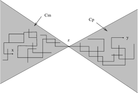
Figure 3. ${\sf z}$ is a cone point of $\mathbf{Cl}({\sf x},{\sf y})$

Clearly, $\mathbf{Cl}({\sf x},{\sf y})$ cannot have any cone points at all once ${\sf y}\not\in{\sf x}+\mathcal{C}_{\delta}$. In the latter case, however,

$$\tau_{p}({\sf y}-{\sf x})>\left\langle t_{p},{\sf y}-{\sf x}\right\rangle+c_{2}\delta|{\sf y}-{\sf x}|,$$

where

$$c_{2}=\min_{{\sf v}\in{\mathbb{S}}^{1}}\frac{\tau_{p}({\sf v})}{|{\sf v}|}.$$

Consequently, there exists ${\color[rgb]{0,0,0}\nu_{0}}={\color[rgb]{0,0,0}\nu_{0}}(p,\delta)>0$ such that

$${\mathbb{B}}_{p}\left(0\longleftrightarrow{\sf x}\right)\,\lesssim\,{\rm e}^{-\left\langle{\sf t}_{p},{\sf x}\right\rangle-{\color[rgb]{0,0,0}\nu_{0}}\lvert{\sf x}\rvert},$$ (2.23)

uniformly in ${\sf x}\not\in\mathcal{C}_{\delta}$.

On the other hand, for ${\sf x}\in\mathcal{C}_{\delta}$, the techniques developed in [CI, CIV1, GI, CIV3] readily imply the following mass-gap type result: For $0<k<m$ and ${\sf x}\in\mathcal{H}_{m}$ consider the event,

$$\mathcal{N}_{k,m}({\sf x})\,\stackrel{{\scriptstyle\Delta}}{{=}}\,\left\{\mathbf{Cl}(0,{\sf x})\ \text{has no cone points in $\mathcal{H}_{k,m}$}\right\}.$$

Then,

Theorem 2.4.

There exists ${\color[rgb]{0,0,0}\nu_{1}}={\color[rgb]{0,0,0}\nu_{1}}(p,\delta)>0$ such that uniformly in $k,l\in{\mathbb{N}}$ and in ${\sf x}\in\mathcal{C}_{\delta}\cap\mathcal{H}_{k+l}$,

$${\mathbb{B}}_{p}\left(0\longleftrightarrow{\sf x}~{};~{}\mathcal{N}_{k,k+l}({\sf x})\right)\,\lesssim\,{\rm e}^{-\left\langle{\sf t}_{p},{\sf x}\right\rangle-{\color[rgb]{0,0,0}\nu_{1}}l}.$$ (2.24)

Proof. A straight forward adaptation of the arguments in  [CI, CIV1, GI, CIV3]. ∎

Together (2.23) and (2.24) imply: There exists ${\color[rgb]{0,0,0}\nu_{2}}={\color[rgb]{0,0,0}\nu_{2}}(p,\delta)>0$, such that uniformly in $l\in{\mathbb{N}}$ and in ${\sf x}\in\mathcal{H}_{l}$,

$$\sum_{k\;\geqslant\;0}{\mathbb{B}}_{p}\left(0\longleftrightarrow{\sf x}+k{\sf e}_{1}~{};~{}\mathcal{N}_{k,k+l}({\sf x}+k{\sf e}_{1})\right)\,\lesssim\,{\rm e}^{-\left\langle{\sf t}_{p},{\sf x}\right\rangle-{\color[rgb]{0,0,0}\nu_{2}}\lvert{\color[rgb]{0,0,0}{\sf x}}\rvert}.$$ (2.25)

Indeed, if ${\sf x}+k{\sf e}_{1}\not\in\mathcal{C}_{\delta}$, then by (2.23),

$${\mathbb{B}}_{p}\left(0\longleftrightarrow{\sf x}+k{\sf e}_{1}\right)\,\lesssim\,{\rm exp}\left\{-\left\langle{\sf t}_{p},{\sf x}+k{\sf e}_{1}\right\rangle-{\color[rgb]{0,0,0}\nu_{0}}\lvert{\sf x}+k{\sf e}_{1}\rvert\right\}\,\;\leqslant\;\,{\rm e}^{-\left\langle{\sf t}_{p},{\sf x}\right\rangle-{\color[rgb]{0,0,0}\nu_{0}}\lvert{\color[rgb]{0,0,0}{\sf x}}\rvert-k\tau_{p}}.$$

If, however, ${\sf x}+k{\sf e}_{1}\in\mathcal{C}_{\delta}$, then

$$\left\langle{\sf t}_{p},k{\sf e}_{1}\right\rangle+{\color[rgb]{0,0,0}\nu_{1}}l~{}\;\geqslant\;~{}{\color[rgb]{0,0,0}\nu_{3}}\left(k+\lvert{\sf x}\rvert\right),$$

for some ${\color[rgb]{0,0,0}\nu_{3}}={\color[rgb]{0,0,0}\nu_{3}}(p,\delta)$, and one can rely on (2.24) in order to conclude that

$${\mathbb{B}}_{p}\left(0\longleftrightarrow{\sf x}+k{\sf e}_{1}~{};~{}\mathcal{N}_{k,k+l}({\sf x})\right)\,\lesssim\,{\rm e}^{-\left\langle{\sf t}_{p},{\sf x}\right\rangle-{\color[rgb]{0,0,0}\nu_{3}}\lvert{\color[rgb]{0,0,0}{\sf x}}\rvert-k{\color[rgb]{0,0,0}\nu_{3}}}.$$

It follows that,

$${\mathbb{B}}_{p}\left(0\longleftrightarrow{\sf x}+k{\sf e}_{1}~{};~{}\mathcal{N}_{k,k+l}({\sf x})\right)\,\lesssim\,{\rm e}^{-\left\langle{\sf t}_{p},{\sf x}\right\rangle-\min\left\{{\color[rgb]{0,0,0}\nu_{0}},{\color[rgb]{0,0,0}\nu_{3}}\right\}\lvert{\color[rgb]{0,0,0}{\sf x}}\rvert-k\min\left\{{\color[rgb]{0,0,0}\nu_{3}},\tau_{p}\right\}},$$ (2.26)

uniformly in $k,l\in{\mathbb{N}}$ and in ${\sf x}\in\mathcal{H}_{l}$ . Summing over $k$ yields 2.25.

2.5. Proof of Lemma 2.3

Recall that $p_{c}=1/2<p^{*}=1-p$ and that the sub-critical $p$-percolation lives on the direct lattice ${\mathbb{Z}}^{2}$ . We claim that there exists ${\color[rgb]{0,0,0}\nu_{4}}={\color[rgb]{0,0,0}\nu_{4}}(p)>0$ such that,

$${\mathbb{B}}_{p}\left(\mathcal{L}([{\sf v},{\sf x}])\right)\,\lesssim\,{\rm exp}\left\{-\left\langle{\sf t}_{p},{\sf v}+{\sf x}\right\rangle-{\color[rgb]{0,0,0}\nu_{4}}\left(|{\sf v}|+|{\sf x}|\right)\right\}$$ (2.27)

uniformly in $l\in{\mathbb{N}}$ and in ${\sf v},{\sf x}\in\mathcal{H}_{l}$. (2.15) is an immediate consequence. In its turn (2.27) is a mass-gap estimate of the same type as (2.25). More precisely, for $k\;\geqslant\;0$ define

$$\mathcal{L}_{-k}([{\sf v},{\sf x}])\,=\,\left(\left\{(-k,0)\longleftrightarrow{\sf v}\right\}\circ\left\{(-k,0)\longleftrightarrow{\sf x}\right\}\right)\cap\mathcal{L}([{\sf v},{\sf x}]).$$

Then, by a more or less straightforward adjustment of the arguments leading to (2.26) we infer that there exists ${\color[rgb]{0,0,0}\nu_{4}=\nu_{4}(p)}$, ${\color[rgb]{0,0,0}\nu_{5}}={\color[rgb]{0,0,0}\nu_{5}}(p)$ such that,

$${\mathbb{B}}_{p}\left(\mathcal{L}_{-k}([{\sf v},{\sf x}])\right)\,\lesssim\,{\rm exp}\left\{-2k\min\left\{\tau_{p},{\color[rgb]{0,0,0}\nu_{5}}\right\}-\left\langle{\sf t}_{p},{\sf v}+{\sf x}\right\rangle-{\color[rgb]{0,0,0}\nu_{4}}\left(|{\sf v}|+|{\sf x}|\right)\right\}.$$

Since,

$${\mathbb{B}}_{p}\left(\mathcal{L}([{\sf v},{\sf x}])\right)\,\;\leqslant\;\,\sum_{k}{\mathbb{B}}_{p}\left(\mathcal{L}_{-k}([{\sf v},{\sf x}])\right),$$

(2.27) follows.∎

2.6. Proof of Lemma 2.1

Lemma 2.1 follows by a very similar line of reasoning:
As in the case of (2.27), mass-gap type estimates of [CI, CIV3] imply that there exists ${\color[rgb]{0,0,0}\nu_{6}}={\color[rgb]{0,0,0}\nu_{6}}(p)>0$, such that

$${\mathbb{B}}_{p}\left(\mathcal{I}([{\sf v},{\sf x}],[{\sf u},{\sf y}])\right)\,\lesssim\,{\rm e}^{-2N\tau_{p}-{\color[rgb]{0,0,0}\nu_{6}}(|{\sf v}|+|{\sf x}|+|{\sf x}_{N}^{*}-{\sf u}|+|{\sf x}_{N}^{*}-{\sf y}|)}\quad\text{and}\quad{\mathbb{B}}_{p}\left(\mathcal{I}(\emptyset)\right)\,\lesssim\,{\rm e}^{-2N(\tau_{p}+{\color[rgb]{0,0,0}\nu_{6}})}.$$

These are a-priori bounds: Once Theorem  2.2 is established they render ${\mathbb{B}}_{p}\left(\mathcal{I}(\emptyset)\right)$ or ${\mathbb{B}}_{p}\left(\mathcal{I}([{\sf v},{\sf x}],[{\sf u},{\sf y}])\right)$, with at least one of $|{\sf v}|,|{\sf x}|,|{\sf x}_{N}^{*}-{\sf u}|,|{\sf x}_{N}^{*}-{\sf y}|$ being $\gtrsim\log N$, negligible with respect to the right hand side of (2.3).∎

3. Reduction to the Effective RW Picture

We continue to assume that ${\sf v},{\sf x}\in\mathcal{H}_{m}$ and ${\sf u},{\sf y}\in\mathcal{H}_{N-r}$, with $m<N-r$. The Lemma below explains the advantage of working with events $\mathcal{A}([{\sf v},{\sf x}],[{\sf u},{\sf y}])$ and, consequently, the reasons behind an introduction of modified events $\widetilde{}\mathcal{I}([{\sf v},{\sf x}],[{\sf u},{\sf y}])$ in (2.11).

Lemma 3.1.

Let $m,r,{\sf v},{\sf x},{\sf u}$ and ${\sf y}$ be as above. Then,

$${\mathbb{B}}_{p}\left(\mathcal{A}([{\sf v},{\sf x}],[{\sf u},{\sf y}])\right)\,=\,\otimes{\mathbb{B}}_{p}\left(\mathcal{A}([{\sf v},{\sf x}],[{\sf u},{\sf y}])\right),$$ (3.1)

where $\otimes{\mathbb{B}}_{p}$ means that the clusters $\mathbf{Cl}_{m,N-r}({\sf x},{\sf y})$ and $\mathbf{Cl}_{m,N-r}({\sf v},{\sf u})$ are sampled independently.

Proof. Let us decompose $\mathcal{A}([{\sf v},{\sf x}],[{\sf u},{\sf y}])$ with respect to realizations of $\gamma^{\rm up}(\mathbf{Cl}_{m,N-r}({\sf x},{\sf y}))$,

$${\mathbb{B}}_{p}\left(\mathcal{A}([{\sf v},{\sf x}],[{\sf u},{\sf y}])\right)\,=\,\sum_{\gamma}{\mathbb{B}}_{p}\left(\mathcal{A}([{\sf v},{\sf x}],[{\sf u},{\sf y}])\,,\,\gamma^{\rm up}(\mathbf{Cl}_{m,N-r}({\sf x},{\sf y}))=\gamma\right).$$

Using $\mathcal{A}([{\sf v},{\sf x}],[{\sf u},{\sf y}])^{\star}$ for $\star=\mathbf{a},\dots\mathbf{e}$ to denote the events described by conditions ${\bf a)}-{\bf e)}$ in the definition of $\mathcal{A}$ in Subsection 2.2, we readily see that

$$\mathcal{A}^{\mathbf{a}}\cap\mathcal{A}^{\mathbf{c}}\cap\{\mathbf{Cl}_{m,N-r}({\sf v},{\sf u})\cap\gamma=\emptyset\}\ \text{and}\ \mathcal{A}^{\mathbf{b}}\cap\mathcal{A}^{\mathbf{d}}\cap\{\gamma^{\rm up}(\mathbf{Cl}_{m,N-r}({\sf x},{\sf y}))=\gamma\}$$

are independent under ${\mathbb{B}}_{p}$.∎

3.1. Decomposition of $\mathcal{A}([{\sf v},{\sf x}],[{\sf u},{\sf y}])$

In light of the previous Lemma, we may calculate probabilities using the product measure. Since we restrict attention to the case $m,r\lesssim\log N$, for the sake of proving Theorem  2.2 we may now assume without loss of generality that $m=r=0$. Thus,

$${\sf v}=(0,v),\ {\sf x}=(0,x),\ {\sf u}=(N,u)\ \text{and}\ {\sf y}=(N,y).$$

Given $0<l<N$ and ${\sf w},{\sf z}\in\mathcal{H}_{l}$ let us say that $\mathcal{H}_{l}$ is a cone cut line and, accordingly, that $\left\{{\sf w},{\sf z}\right\}$ is a cone couple for $\left\{\mathbf{Cl}_{0,N}({\sf v},{\sf u}),\mathbf{Cl}_{0,N}({\sf x},{\sf y})\right\}$ if ${\sf w}$ is a cone point of $\mathbf{Cl}_{0,N}({\sf v},{\sf u})$, whereas ${\sf z}$ is a cone point of $\mathbf{Cl}_{0,N}({\sf x},{\sf y})$.

A straightforward adjustment of the renormalization arguments behind (2.24) in [CI, CIV1, CIV3] implies that there exist ${\color[rgb]{0,0,0}\nu_{7}}={\color[rgb]{0,0,0}\nu_{7}}(p,\delta)>0$, such that,

$$\begin{split}&\otimes{\mathbb{B}}_{p}\left(\left\{\mathbf{Cl}_{0,N}({\sf v},{\sf u}),\mathbf{Cl}_{0,N}({\sf x},{\sf y})\right\}\,\text{has less than two cone cut lines}\right)\,\\ &\qquad\lesssim\,{\rm e}^{-\left\langle{\sf t}_{p},{\sf u}-{\sf v}\right\rangle-\left\langle{\sf t}_{p},{\sf y}-{\sf x}\right\rangle-{\color[rgb]{0,0,0}\nu_{7}}N}\end{split}$$ (3.2)

uniformly in ${\sf v},{\sf x},{\sf u}$ and ${\sf y}$ under consideration. In the case when $\left\{\mathbf{Cl}_{0,N}({\sf v},{\sf u}),\mathbf{Cl}_{0,N}({\sf x},{\sf y})\right\}$ has at least two cone cut lines, say $l_{1},\dots,l_{n+1}$ with

$$\left\{{\sf w}_{1}=(l_{1},w_{1}),{\sf z}_{1}=(l_{1},z_{1})\right\},\dots,\left\{{\sf w}_{n+1}=(l_{n+1},w_{n+1}),{\sf z}_{n+1}=(l_{n+1},z_{n+1}\right\}$$

being the corresponding cone couples, there is a simultaneous irreducible decomposition (see Figure 4),

$$\mathbf{Cl}_{0,N}({\sf v},{\sf u})\,=\,\Gamma_{b}^{1}\cup\Gamma_{1}^{1}\cup\dots\cup\Gamma_{n}^{1}\cup\Gamma_{f}^{1}\quad\text{and}\quad\mathbf{Cl}_{0,N}({\sf x},{\sf y})\,=\,\Gamma_{b}^{2}\cup\Gamma_{1}^{2}\cup\dots\cup\Gamma_{n}^{2}\cup\Gamma_{f}^{2}.$$ (3.3)

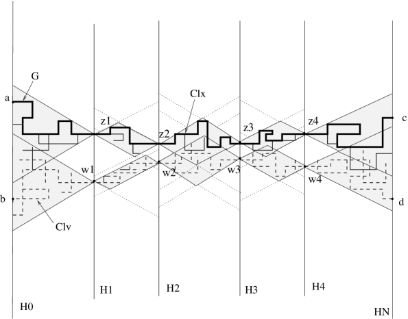
Figure 4. Decomposition of $\mathcal{A}([{\sf v},{\sf x}],[{\sf u},{\sf y}])$: $l_{1},l_{2},l_{3},l_{4}$ are cut lines.
$\left\{{\sf w}_{1},{\sf z}_{1}\right\},\left\{{\sf w}_{2},{\sf z}_{2}\right\},\left\{{\sf w}_{3},{\sf z}_{3}\right\},\left\{{\sf w}_{4},{\sf z}_{4}\right\}$ are the corresponding cone couples

The simultaneous irreducible decomposition (3.3) sets up the stage for our effective random walk representation of the double cluster $\left\{\mathbf{Cl}_{0,N}({\sf v},{\sf u}),\mathbf{Cl}_{0,N}({\sf x},{\sf y})\right\}$. In fact, our effective random walk will just run through the cone couples of the latter. We, therefore, proceed with a careful description of clusters and associated irreducible events which show up in (3.3)

3.2. Irreducible pairs and associated events

We shall consider the following families of clusters:

Initial clusters

For $l>0$ and ${\sf w},{\sf z}\in\mathcal{H}_{l}$, let $\mathcal{F}_{b}([{\sf w},{\sf z}])$ be the set of cluster pairs $\left(\Gamma_{b}^{1},\Gamma_{b}^{2}\right)$ satisfying:
(i) $\Gamma_{b}^{i}\subseteq\mathcal{H}_{0,l}$ for $i=1,2$.

(ii) $\max\left\{\Gamma_{b}^{1}\cap\mathcal{H}_{0}\right\}=\max\left\{\Gamma_{b}^{2}\cap\mathcal{H}_{0}\right\}=\left\{0\right\}$ .

(iii) $\Gamma_{b}^{1}\cap\mathcal{H}_{l}=\left\{{\sf w}\right\}$ and $\Gamma_{b}^{2}\cap\mathcal{H}_{l}=\left\{{\sf z}\right\}$.

(iv) $\Gamma_{b}^{1}\subseteq{\sf w}-\mathcal{C}_{\delta}$ and $\Gamma_{b}^{2}\subseteq{\sf z}-\mathcal{C}_{\delta}$.

(v) $\forall k=1,\dots,l-1$, $\,\mathcal{H}_{k}$ is not a cone cut line for $\left(\Gamma_{b}^{1},\Gamma_{b}^{2}\right)$ in $\mathcal{H}_{0,l}$ (irreducibility).

For each such pair of clusters, with a slight abuse of notation we proceed to denote by $\left\{\Gamma_{b}^{1},\Gamma_{b}^{2}\right\}$ the $\mathfrak{E}^{-}_{0,l}\times\mathfrak{E}^{-}_{0,l}$-measurable event that

$$\left\{\mathbf{Cl}^{-}_{0,l}(0,{\sf w})=\Gamma_{b}^{1}\right\}\times\left\{\mathbf{Cl}^{-}_{0,l}(0,{\sf z})=\Gamma_{b}^{2}\right\}.$$

Finally let:

$$\mathcal{F}_{b}=\bigcup_{l\;\geqslant\;1}\bigcup_{{\sf w},{\sf z}\in\mathcal{H}_{l}}\mathcal{F}_{b}([{\sf w},{\sf z}])$$

In the sequel we define random steps $\sigma_{b}=\left(\rho_{b},\xi_{b}^{1},\xi_{b}^{2}\right):\mathcal{F}_{b}\mapsto{\mathbb{Z}}_{+}\times{\mathbb{Z}}^{2}$: If $l>0$; ${\sf w}=(l,w)$, ${\sf z}=(l,z)$ and $\left(\Gamma_{b}^{1},\Gamma_{b}^{2}\right)\in\mathcal{F}_{b}\left([{\sf w},{\sf z}]\right)$, then

$$\sigma_{b}(\Gamma_{b}^{1},\Gamma_{b}^{2})=\left(\rho_{b},\xi_{b}^{1},\xi_{b}^{2}\right)=\left(l,w,z\right).$$

Bulk clusters

For $l>0$ and ${\sf w},{\sf z}\in\mathcal{H}_{l}$, let $\mathcal{F}([{\sf w},{\sf z}])$ be the set of cluster pairs $\left(\Gamma^{1},\Gamma^{2}\right)$ satisfying:

(i) $\Gamma^{i}\subseteq\mathcal{H}_{0,l}$ for $i=1,2$.

(ii) $\Gamma^{1}\cap\mathcal{H}_{0}=\Gamma^{2}\cap\mathcal{H}_{0}=\left\{0\right\}$

(iii) $\Gamma^{1}\cap\mathcal{H}_{l}=\left\{{\sf w}\right\}$ and $\Gamma^{2}\cap\mathcal{H}_{l}=\left\{{\sf z}\right\}$.

(iv) $\Gamma^{1}\subseteq\mathcal{C}_{\delta}\cap\left({\sf w}-\mathcal{C}_{\delta}\right)$ and $\Gamma^{2}\subseteq\mathcal{C}_{\delta}\cap\left({\sf z}-\mathcal{C}_{\delta}\right)$ .

(v) $\forall k=1,\dots,l-1$, $\,\mathcal{H}_{k}$ is not a cone cut line for $\left(\Gamma^{1},\Gamma^{2}\right)$ in $\mathcal{H}_{0,l}$ (irreducibility).

For each such pair of clusters, with a slight abuse of notation we proceed to denote by $\left\{\Gamma^{1},\Gamma^{2}\right\}$ the $\mathfrak{E}^{-}_{0,l}\times\mathfrak{E}^{-}_{0,l}$-measurable event that

$$\left\{\mathbf{Cl}^{-}_{0,l}(0,{\sf w})=\Gamma^{1}\right\}\times\left\{\mathbf{Cl}^{-}_{0,l}(0,{\sf z})=\Gamma^{2}\right\}.$$

Finally let:

$${\color[rgb]{0,0,0}\mathcal{F}}=\bigcup_{l\;\geqslant\;1}\bigcup_{{\sf w},{\sf z}\in\mathcal{H}_{l}}\mathcal{F}([{\sf w},{\sf z}])$$

In the sequel we define random steps $\sigma=\left(\rho,\xi^{1},\xi^{2}\right):\mathcal{F}\mapsto{\mathbb{Z}}_{+}\times{\mathbb{Z}}^{2}$: If $l>0$; ${\sf w}=(l,w)$, ${\sf z}=(l,z)$ and $\left(\Gamma^{1},\Gamma^{2}\right)\in\mathcal{F}\left([{\sf w},{\sf z}]\right)$, then

$$\sigma(\Gamma^{1},\Gamma^{2})=\left(\rho,\xi^{1},\xi^{2}\right)=\left(l,w,z\right).$$

Terminal clusters

For $l>0$ and ${\sf w},{\sf z}\in\mathcal{H}_{l}$, let $\mathcal{F}_{{\color[rgb]{0,0,0}f}}([{\sf w},{\sf z}])$ be the set of cluster pairs $\left(\Gamma_{f}^{1},\Gamma_{f}^{2}\right)$ satisfying:

(i) $\Gamma_{f}^{i}\subseteq\mathcal{H}_{0,l}$ for $i=1,2$.

(ii) $\Gamma_{f}^{1}\cap\mathcal{H}_{0}=\Gamma_{f}^{2}\cap\mathcal{H}_{0}=\left\{0\right\}$.

(iii) $\max\left\{\Gamma_{f}^{1}\cap\mathcal{H}_{l}\right\}=\left\{{\sf w}\right\}$ and $\max\left\{\Gamma_{f}^{2}\cap\mathcal{H}_{l}\right\}=\left\{{\sf z}\right\}$.

(iv) $\Gamma_{f}^{1}\subseteq\mathcal{C}_{\delta}\quad$ and $\Gamma_{f}^{2}\subseteq\mathcal{C}_{\delta}$.

(v) $\forall k=1,\dots,l-1$, $\,\mathcal{H}_{k}$ is not a cone cut line for $\left(\Gamma_{f}^{1},\Gamma_{f}^{2}\right)$ in $\mathcal{H}_{0,l}$ (irreducibility).

For each such pair of clusters, with a slight abuse of notation we proceed to denote by $\left\{\Gamma_{f}^{1},\Gamma_{f}^{2}\right\}$ the $\mathfrak{E}_{0,l}\times\mathfrak{E}_{0,l}$-measurable event that

$$\left\{\mathbf{Cl}_{0,l}(0,{\sf w})=\Gamma_{f}^{1}\right\}\times\left\{\mathbf{Cl}_{0,l}(0,{\sf z})=\Gamma_{f}^{2}\right\}.$$

Finally let:

$$\mathcal{F}_{f}=\bigcup_{l\;\geqslant\;1}\bigcup_{{\sf w},{\sf z}\in\mathcal{H}_{l}}\mathcal{F}_{f}([{\sf w},{\sf z}],)$$

In the sequel we define random steps $\sigma_{f}=\left(\rho_{f},\xi^{1}_{f},\xi^{2}_{f}\right):\mathcal{F}_{{\color[rgb]{0,0,0}f}}\mapsto{\mathbb{Z}}_{+}\times{\mathbb{Z}}^{2}$: If $l>0$; ${\sf w}=(l,w)$, ${\sf z}=(l,z)$ and $\left(\Gamma_{{\color[rgb]{0,0,0}f}}^{1},\Gamma_{{\color[rgb]{0,0,0}f}}^{2}\right)\in\mathcal{F}_{{\color[rgb]{0,0,0}f}}\left([{\sf w},{\sf z}]\right)$, then

$$\sigma_{f}(\Gamma_{{\color[rgb]{0,0,0}f}}^{1},\Gamma_{{\color[rgb]{0,0,0}f}}^{2})=\left(\rho_{f},\xi^{1}_{f},\xi^{2}_{f}\right)=\left(l,w,z\right).$$

3.3. Construction of the effective random walk

Let us fix:

1) A pair of intial clusters $\left(\widetilde{\Gamma}_{b}^{1},\widetilde{\Gamma}_{b}^{2}\right)\in\mathcal{F}_{b}$.

2) A sequence of pairs of clusters $\left((\widetilde{\Gamma}_{k}^{1},\widetilde{\Gamma}_{k}^{2})\right)_{{\color[rgb]{0,0,0}{k\;\geqslant\;1}}}\subset\mathcal{F}$.

3) A pair of terminal clusters $\left(\widetilde{\Gamma}_{f}^{1},\widetilde{\Gamma}_{f}^{2}\right)\in\mathcal{F}_{f}$.

For $n>0$ and ${\sf v}=(0,v),{\sf x}=(0,x)$ we construct $n$-step trajectories of the induced effective random walk which starts at $\left\{{\sf v},{\sf x}\right\}$ as follows: By definition,

$$\begin{split}&S_{0}\stackrel{{\scriptstyle\Delta}}{{=}}(T_{0},V_{0},X_{0})=(0,v,x),\quad S_{k}\stackrel{{\scriptstyle\Delta}}{{=}}(T_{k},V_{k},X_{k})=S_{0}+\sum_{1}^{k}\sigma_{l},\\ &S_{k}^{b}\stackrel{{\scriptstyle\Delta}}{{=}}(T_{k}^{b},V_{k}^{b},X_{k}^{b})=\sigma_{b}+S_{k},\quad S_{k}^{f}\stackrel{{\scriptstyle\Delta}}{{=}}(T_{k}^{f},V_{k}^{f},X_{k}^{f})=S_{k}+\sigma_{f},\\[4.30554pt] &S_{n}^{bf}\stackrel{{\scriptstyle\Delta}}{{=}}(T_{n}^{bf},V_{n}^{bf},X_{n}^{bf})=\sigma_{b}+S_{n}+\sigma_{f},\end{split}$$ (3.4)

Above,

$$\sigma_{b}=\sigma_{b}\left(\widetilde{\Gamma}_{b}^{1},\widetilde{\Gamma}_{b}^{2}\right),\ \sigma_{k}=\sigma\left(\widetilde{\Gamma}_{k}^{1},\widetilde{\Gamma}_{k}^{2}\right)\quad\text{and}\quad\sigma_{f}=\sigma_{f}\left(\widetilde{\Gamma}_{f}^{1},\widetilde{\Gamma}_{f}^{2}\right).$$

Let $N>0$, $u,y\in\mathcal{H}_{N}$ such that $S_{n}^{bf}=(N,u,y)$. Set also ${\sf u}=(N,u)$, ${\sf y}=(N,y)$. In this notations, ${\color[rgb]{0,0,0}S_{0}},S_{0}^{b},S_{1}^{b},\dots,S_{n}^{b},S_{n}^{bf}=S_{n}^{b}+\sigma_{f}$ describes interpolated trajectories through cone cut points of the simultaneous irreducible decomposition of pair of clusters,

$$\Gamma_{b}^{1}\cup\Gamma_{1}^{1}\cup\dots\cup\Gamma_{n}^{1}\cup\Gamma_{f}^{1}\quad\text{and}\quad\Gamma_{b}^{2}\cup\Gamma_{1}^{2}\cup\dots\cup\Gamma_{n}^{2}\cup\Gamma_{f}^{2},$$ (3.5)

where the induced clusters are defined as follows:

$$\begin{split}&\left(\Gamma_{b}^{1},\Gamma_{b}^{2}\right)=\left({\sf v}+\widetilde{\Gamma}_{b}^{1},{\sf x}+\widetilde{\Gamma}_{b}^{2}\right),\\ &\left(\Gamma_{k}^{1},\Gamma_{k}^{2}\right)=\left((T^{b}_{k-1},V^{b}_{k-1})+\widetilde{\Gamma}_{k}^{1},\,(T^{b}_{k-1},X^{b}_{k-1})+\widetilde{\Gamma}_{k}^{2}\right),\\ &\left(\Gamma_{f}^{1},\Gamma_{f}^{2}\right)=\left((T^{b}_{n},V^{b}_{n})+\widetilde{\Gamma}_{f}^{1},\,(T^{b}_{n},X^{b}_{n})+\widetilde{\Gamma}_{f}^{2}\right).\end{split}$$

Comparing (3.5) with (3.3) we see that in particular the above procedure generates distinctly all the cluster pairs which contribute to the events $\mathcal{A}\left([{\sf v},{\sf x}],[{\sf u},{\sf y}]\right)$ (and which have at least two cone cut lines, of course).

Let us indroduce now the weights,

$$\begin{split}&\widetilde{{\mathbb{B}}}_{p}^{v,x}\left(\Gamma_{b}^{1}\cup\Gamma_{1}^{1}\cup\dots\cup\Gamma_{n}^{1}\cup\Gamma_{f}^{1};\Gamma_{b}^{2}\cup\Gamma_{1}^{2}\cup\dots\cup\Gamma_{n}^{2}\cup\Gamma_{f}^{2}\right)\\ &=\otimes{\mathbb{B}}_{p}\left(\left\{\widetilde{\Gamma}^{1}_{b},\widetilde{\Gamma}^{2}_{b}\right\}\right)\prod_{1}^{n}\otimes{\mathbb{B}}_{p}\left(\left\{\widetilde{\Gamma}^{1}_{k},\widetilde{\Gamma}^{2}_{k}\right\}\right)\otimes{\mathbb{B}}_{p}\left(\left\{\widetilde{\Gamma}^{1}_{f},\widetilde{\Gamma}^{2}_{f}\right\}\right),\end{split}$$

and the events,

$$\widetilde{\mathcal{A}}([{\sf v},{\sf x}],[{\sf u},{\sf y}])=\bigcup_{n{\color[rgb]{0,0,0}\;\geqslant\;}1}\left\{S_{n}^{bf}=(N,u,y);\quad\Gamma^{1}_{k}\cap\gamma^{\rm up}(\Gamma^{2}_{k})=\emptyset\quad\text{for}\,k=b,1,\dots,n,f\right\}.$$ (3.6)

Then the irreducibility of decomposition (3.3) together with (3.2) imply that we can express the probability of percolation event $\mathcal{A}([{\sf v},{\sf x}],[{\sf u},{\sf y}])$ under $\otimes{\mathbb{B}}_{p}$ asymptotically as the probability of “clusters-random-walk” event $\widetilde{\mathcal{A}}([{\sf v},{\sf x}],[{\sf u},{\sf y}])$ under $\widetilde{{\mathbb{B}}}_{p}^{v,x}$:

$$\otimes{\mathbb{B}}_{p}\left(\mathcal{A}([{\sf v},{\sf x}],[{\sf u},{\sf y}])\right)\left(1+{\small O}\left({\rm e}^{-{\color[rgb]{0,0,0}\nu_{7}}N}\right)\right)=\widetilde{{\mathbb{B}}}_{p}^{v,x}\left(\widetilde{\mathcal{A}}([{\sf v},{\sf x}],[{\sf u},{\sf y}])\right).$$ (3.7)

Furthermore, if we set

$$\mathcal{R}_{n}^{bf}\,\stackrel{{\scriptstyle\Delta}}{{=}}\,\left\{X_{0}^{b}>V_{0}^{b}\right\}\cap\left\{X_{k}^{b}>V_{k}^{b}:\,k=1,\,\dots,\,n\right\}\cap\left\{X_{n}^{bf}>V_{n}^{bf}\right\}$$ (3.8)

we can write

$$\begin{split}&\widetilde{{\mathbb{B}}}_{p}^{v,x}\left(\widetilde{\mathcal{A}}([{\sf v},{\sf x}],[{\sf u},{\sf y}])\right)\\ &=\,\sum_{n{\color[rgb]{0,0,0}\;\geqslant\;}1}\widetilde{{\mathbb{B}}}_{p}^{v,x}\left(S_{n}^{bf}=(N,u,y)\,;\,\mathcal{R}_{n}^{bf}\right)\,\widetilde{{\mathbb{B}}}_{p}^{v,x}\left(\widetilde{\mathcal{A}}([{\sf v},{\sf x}],[{\sf u},{\sf y}])\,\big{|}\,S_{n}^{bf}=(N,u,y)\,;\,\mathcal{R}_{n}^{bf}\right).\end{split}$$ (3.9)

We shall argue that the conditional probability above leads only to finite corrections, whereas sharp asymptotics are inherited from $\widetilde{{\mathbb{B}}}_{p}^{v,x}\left(S_{n}^{bf}=(N,u,y)\,;\ \mathcal{R}_{n}^{bf}\right)$ terms. This is a reduction to the effective random walk picture as described in Subsection 1.

3.4. Normalized step distributions

Bulk steps

We shall now fix the steps of our effective random walk, making their distribution proper and check that this distribution satisifies conditions (P1)-(P3) of Subsection 1 whence we can use Theorem B. Let us introduce yet another probability measure ${\mathbb{P}}_{v,x}$ under which $(\sigma_{k})_{k\;\geqslant\;1}$ form an infinite collection of independent random variables that share a common distribution defined as follows:

$${\mathbb{P}}_{v,x}\left(\sigma=(r,x_{1},x_{2})\right)\,=\,{\rm e}^{2r\tau_{p}}\widetilde{{\mathbb{B}}}_{p}^{v,x}\left(\sigma_{1}=(r,x_{1},x_{2})\right)\,=\,{\rm e}^{2r\tau_{p}}\sum_{\left(\Gamma^{1},\Gamma^{2}\right)}\otimes{\mathbb{B}}_{p}\left(\left\{\Gamma^{1},\Gamma^{2}\right\}\right),$$ (3.10)

where the summation is over all pairs $\left(\Gamma^{1},\Gamma^{2}\right)\in\mathcal{F}([(r,x_{1}),(r,x_{2})])$. We claim that $\sigma$ is a proper random variable under ${\mathbb{P}}_{v,x}$:

$$\sum_{(r,x_{1},x_{2})}{\mathbb{P}}_{v,x}\left(\sigma=(r,x_{1},x_{2})\right)\,=\,1.$$ (3.11)

Recall the notation ${\sf t}_{p}=(\tau_{p},0)=\tau_{p}({\sf e}_{1})$. Thus $r\tau_{p}$ equals to $\left\langle{\sf t}_{p},(r,x_{i})\right\rangle$ for $i=1,2$. For $l\;\leqslant\;r$ let us say that two points ${\sf w}\in\mathcal{H}_{l}$ and ${\sf z}\in\mathcal{H}_{r}$ are $c$-connected, ${\sf w}\stackrel{{\scriptstyle{c}}}{{\longleftrightarrow}}{\sf z}$ if $\mathbf{Cl}_{l,r}^{-}({\sf w},{\sf z})\neq\emptyset$ and, in addition,

$$\mathbf{Cl}_{l,r}^{-}({\sf w},{\sf z})\,\subseteq\,\left({\sf w}+\mathcal{C}_{\delta}\right)\cap\left({\sf z}-\mathcal{C}_{\delta}\right).$$

The event $\left\{{\sf w}\stackrel{{\scriptstyle{c}}}{{\longleftrightarrow}}{\sf z}\right\}$ is $\mathfrak{E}_{l,r}^{-}$-measurable. The results of [CI, CIV3] imply the following consequence of (2.18) : There exists a neighbourhood $\mathcal{U}$ of ${\sf t}_{p}\in\partial{\bf K}_{p}$, such that for every ${\sf t}\in\mathcal{U}$,

$$\sum_{{\sf z}}{\rm e}^{\left\langle{\sf t},{\sf z}\right\rangle}\,{\mathbb{B}}_{p}\left(0\stackrel{{\scriptstyle{c}}}{{\longleftrightarrow}}{\sf z}\right)\,<\,\infty\ \Longleftrightarrow\ {\sf t}\in\text{int}\left({\bf K}_{p}\right).$$

As a result, for every ${\sf t}\in\text{int}\left({\bf K}_{p}\right)\cap\mathcal{U}$, there exists $\alpha>0$, such that

$$\sum_{{\sf z}\in\mathcal{H}_{r}}{\rm e}^{\left\langle{\sf t},{\sf z}\right\rangle}\,{\mathbb{B}}_{p}\left(0\stackrel{{\scriptstyle{c}}}{{\longleftrightarrow}}{\sf z}\right)\,\lesssim\,{\rm e}^{-\alpha r}.$$ (3.12)

Conversly, for every ${\sf t}\in\text{ext}\left({\bf K}_{p}\right)\cap\mathcal{U}$, there exists $\alpha>0$, such that

$$\sum_{{\sf z}\in\mathcal{H}_{r}}{\rm e}^{\left\langle{\sf t},{\sf z}\right\rangle}\,{\mathbb{B}}_{p}\left(0\stackrel{{\scriptstyle{c}}}{{\longleftrightarrow}}{\sf z}\right)\,\gtrsim\,{\rm e}^{\alpha r}.$$ (3.13)

At this point we can readily extend these convergence results to double clusters: There exists a possibly smaller neighbourhood $\mathcal{V}\subseteq\mathcal{U}$ of ${\sf t}_{p}\in\partial{\bf K}_{p}$, such that for every ${\sf t}\in\mathcal{V}$,

$$\phi({\sf t})\,\stackrel{{\scriptstyle\Delta}}{{=}}\,\sum_{r>0}\,\sum_{{\sf w},{\sf z}\in\mathcal{H}_{r}}{\rm e}^{\left\langle{\sf t},{\sf w}+{\sf z}\right\rangle}\,\otimes{\mathbb{B}}_{p}\left(0\stackrel{{\scriptstyle{c}}}{{\longleftrightarrow}}{\sf w},0\stackrel{{\scriptstyle{c}}}{{\longleftrightarrow}}{\sf z}\right)\,<\,\infty\ \Longleftrightarrow\ {\sf t}\in\text{int}\left({\bf K}_{p}\right).$$ (3.14)

Define now,

$$g({\sf t})\,=\,\sum_{r>0}\,\sum_{{\sf w},{\sf z}\in\mathcal{H}_{r}}{\rm e}^{\left\langle{\sf t},{\sf w}+{\sf z}\right\rangle}\sum_{\left(\Gamma^{1},\Gamma^{2}\right)}\otimes{\mathbb{B}}_{p}\left(\left\{\Gamma^{1},\Gamma^{2}\right\}\right),$$

where for each $\{{\sf w},{\sf z}\}$ fixed the last summation is over all irreducible pairs $\left(\Gamma^{1},\Gamma^{2}\right)\in\mathcal{F}({\color[rgb]{0,0,0}[{\sf w},{\sf z}]})$. By (3.2) $g$ converges everywhere on $\mathcal{V}$ (once $\mathcal{V}$ is small enough). On the other hand, for ${\sf t}\in\mathcal{V}\cap\text{int}\left({\bf K}_{p}\right)$, functions $\phi$ and $g$ satisfy the renewal relation,

$$\phi({\sf t})\,=\,\frac{g({\sf t})}{1-g({\sf t})}.$$

Consequently $g({\sf t})=1$ is a parametrization of $\partial{\bf K}_{p}\cap\mathcal{V}$. (3.11) follows. ∎

The distribution of $\sigma$ in (3.10) is clearly symmetric in the sense of condition (P3) of Subsection 1. Condition (P1) follows from Property (iv) of bulk clusters, as described in Subsection 3.2. Finally, condition (P2) is satisfied by virtue of (3.2).

Initial and terminal steps

Analogously, we define $\sigma_{b}$, $\sigma_{f}$ to have the following distribution under ${\mathbb{P}}_{v,x}$ independently of all other random variables:

$${\mathbb{P}}_{v,x}(\sigma_{b}=(r,x_{1},x_{2})) \stackrel{{\scriptstyle\Delta}}{{=}} {\mathbb{Q}}_{b}(r,x_{1},x_{2})\,\stackrel{{\scriptstyle\sim}}{{=}}\,{\rm e}^{2r\tau_{p}}\widetilde{{\mathbb{B}}}_{p}^{v,x}(\sigma_{b}=(r,x_{1},x_{2}))$$ (3.15)

$$= {\rm e}^{2r\tau_{p}}\sum_{\left(\Gamma_{b}^{1},\Gamma_{b}^{2}\right)}\otimes{\mathbb{B}}_{p}\left(\left\{\Gamma_{b}^{1},\Gamma_{b}^{2}\right\}\right)$$

and, respectively

$${\mathbb{P}}_{v,x}(\sigma_{f}=(r,x_{1},x_{2})) \stackrel{{\scriptstyle\Delta}}{{=}} {\mathbb{Q}}_{f}(r,x_{1},x_{2})\,\stackrel{{\scriptstyle\sim}}{{=}}\,{\rm e}^{2r\tau_{p}}\widetilde{{\mathbb{B}}}_{p}^{v,x}(\sigma_{f}=(r,x_{1},x_{2}))$$ (3.16)

$$= {\rm e}^{2r\tau_{p}}\sum_{\left(\Gamma_{f}^{1},\Gamma_{f}^{2}\right)}\otimes{\mathbb{B}}_{p}\left(\left\{\Gamma_{f}^{1},\Gamma_{f}^{2}\right\}\right),$$

where the summation is over all initial irreducible pairs $\left(\Gamma^{1}_{b},\Gamma^{2}_{b}\right)\in\mathcal{F}_{b}\left([(r,x_{1}),(r,x_{2})]\right)$ and, respectively, over all terminal irreducible pairs $\left(\Gamma^{1}_{f},\Gamma^{2}_{f}\right)\in\mathcal{F}_{f}\left([(r,x_{1}),(r,x_{2})]\right)$. By definition the $\stackrel{{\scriptstyle\sim}}{{=}}$ relations in (3.15) (3.16) are tuned in such a way that both ${\mathbb{Q}}_{b}$ and ${\mathbb{Q}}_{f}$ become probability measures. In addition, as it follows from (3.2), both display exponential tails. In particular,

$$\sum_{r}\sum_{x_{1},x_{2}}{\mathbb{Q}}_{b}(r,x_{1},x_{2})\,=\,1\quad\text{and}\quad\sum_{r}\sum_{x_{1},x_{2}}{\mathbb{Q}}_{f}(r,x_{1},x_{2})\,=\,1$$ (3.17)

converge exponentially fast in all the arguments.

Trajectories

To complete the setup, we carry over to ${\mathbb{P}}_{v,x}$ the definitions in (3.4) and note that under ${\mathbb{P}}_{v,x}$, $(S_{k})_{k\;\geqslant\;0}$ and $(\sigma_{l})_{l\;\geqslant\;1}$ satisfy the conditions preceding Theorem B. Moreover, the following holds:

$${\rm e}^{2N\tau_{p}}\widetilde{{\mathbb{B}}}_{p}^{v,x}\left((S^{b}_{0},\,S^{b}_{1},\,\dots,\,S^{b}_{n},\,S^{bf}_{n})=\underline{s}\right)\,\stackrel{{\scriptstyle\sim}}{{=}}\,{\mathbb{P}}_{v,x}\left((S^{b}_{0},\,S^{b}_{1},\,\dots,\,S^{b}_{n},\,S^{bf}_{n})=\underline{s}\right)$$ (3.18)

for any trajectory $\underline{s}$ ending at time $N$. We shall use ${\mathbb{P}}$ as a short-hand notation for ${\mathbb{P}}_{0,0}$.

Remark 3.2.

We would like to argue that ${\mathbb{Q}}_{b}(r,x_{1},x_{2})={\mathbb{Q}}_{f}(r,-x_{1},-x_{2})$. This does not follow immediately from symmetry with respect to reflection, since in fact, events in summation (3.15) are $\mathfrak{E}^{-}_{0,r}\times\mathfrak{E}^{-}_{0,r}$-measurable while events in summation (3.16) are from $\mathfrak{E}_{0,r}\times\mathfrak{E}_{0,r}$ - hence not entirely symmeteric. Nevertheless, $\otimes{\mathbb{B}}_{p}$-probabilities of corresponding events in the two summations differ only by a constant factor $(1-p)^{4}$ and thus after the $\stackrel{{\scriptstyle\sim}}{{=}}$ normalization this difference disappears.

3.5. Proof of Theorem 2.2

Let us go back to (3.9). Let $\mu={\mathbb{E}}\rho$ be the expected value of the time coordinate displacement along an irreducible step (under distribution (3.10)). First of all note that one can restrict attention to values of $n$ which satisfy $|N-n\mu|\lesssim\sqrt{N\log N}$ . Indeed, as it easily follows from local limit computations for $K$ sufficiently large,

$$\sum_{n:|N-n\mu|>K\sqrt{N\log N}}{\mathbb{P}}\left(\rho_{1}+\dots+\rho_{n}=N\right)\,=\,{\small o}\left(\frac{1}{N^{2}}\right),$$ (3.19)

which is negligible with respect to the right hand side of (2.14).

For $n$-s in the band $n\mu\in[N-K\sqrt{N\log N},N+K\sqrt{N\log N}]$ and $|v|,|x|,|u|,|y|\lesssim\log N$ we proceed as follows:

Term $\widetilde{{\mathbb{B}}}_{p}^{v,x}\left(S_{n}^{bf}=(N,u,y);\mathcal{R}_{n}^{bf}\right)$

This is a purely random walk term. In view of (3.18)

$$\begin{split}&{\rm e}^{2\tau_{p}N}\widetilde{{\mathbb{B}}}_{p}^{v,x}\left(S_{n}^{bf}=(N,u,y);\mathcal{R}_{n}^{bf}\right)\,\stackrel{{\scriptstyle\sim}}{{=}}{\mathbb{P}}_{v,x}\left(S_{n}^{bf}=(N,u,y);\mathcal{R}_{n}^{bf}\right)\\ &\ \ \stackrel{{\scriptstyle\sim}}{{=}}\,\sum_{l,r>0}\sum_{w_{1}<z_{1}}\sum_{w_{n+1}<z_{n+1}}{\mathbb{Q}}_{b}(l,w_{1}-v,z_{1}-x)\\ &\quad\qquad\quad\quad\ \qquad\qquad\qquad\times{\mathbb{P}}_{w_{1},z_{1}}\left(S_{n}=(N-r-l,w_{n+1},z_{n+1})\,;\,\mathcal{R}_{n}^{+}\right)\\ &\quad\qquad\qquad\qquad\qquad\qquad\qquad\ \ \times{\mathbb{Q}}_{f}(r,u-w_{n+1},y-z_{n+1}).\end{split}$$ (3.20)

In view of the exponential tails of ${\mathbb{Q}}_{b}$ and ${\mathbb{Q}}_{f}$ and Remark 3.2, it is now a straightforward consequence of Theorem B that

$$\begin{split}\sum_{n}{\mathbb{P}}_{v,x}\left(S_{n}^{bf}=(N,u,y);\mathcal{R}_{n}^{bf}\right)\,&\sim\,\frac{1}{N^{2}}\sum_{l}\sum_{v^{\prime}<x^{\prime}}{\mathbb{Q}}_{b}(l,v^{\prime}-v,x^{\prime}-x)U(x^{\prime}-v^{\prime})\\ &\ \times\sum_{r}\sum_{u^{\prime}<y^{\prime}}U(y^{\prime}-u^{\prime}){\mathbb{Q}}_{f}(r,u-u^{\prime},y-y^{\prime})\\ &\stackrel{{\scriptstyle\Delta}}{{=}}\,\frac{\widetilde{U}(x-v)\widetilde{U}(y-u)}{N^{2}}\end{split}$$ (3.21)

uniformly in $|v|,|x|,|u|,|y|\lesssim\log N$.

Term $\widetilde{{\mathbb{B}}}_{p}^{v,x}\left(\widetilde{\mathcal{A}}([{\sf v},{\sf x}],[{\sf u},{\sf y}])\,\big{|}\,S_{n}^{bf}=(N,u,y)\,;\,\mathcal{R}_{n}^{bf}\right)$

We would like to argue that under $\mathcal{R}_{n}^{bf}$ the trajectories of upper and lower random walks are repulsed and, consequently, the additional constraint $\mathbf{Cl}_{0,N}({\sf v},{\sf u})\cap\gamma^{\rm up}(\mathbf{Cl}_{0,N}({\sf x},{\sf y}))$ imposed by the event $\widetilde{\mathcal{A}}([{\sf v},{\sf x}],[{\sf u},{\sf y}])$ actually applies only close to the $\mathcal{H}_{0}$ and $\mathcal{H}_{N}$ lines and, furthermore, this constraint asymptotically decouple. In fact, we claim:

Lemma 3.3.

There exists a positive function $H$ on ${\mathbb{Z}}$ of an at most linear growth; $H(z)\lesssim z$, such that

$$\widetilde{{\mathbb{B}}}_{p}^{v,x}\left(\widetilde{\mathcal{A}}([{\sf v},{\sf x}],[{\sf u},{\sf y}])\,\big{|}\,S_{n}^{bf}=(N,u,y)\,;\,\mathcal{R}_{n}^{bf}\right)\,\sim\,H(x-v)H(y-u)$$ (3.22)

uniformly in $|v|,|x|,|u|,|y|\lesssim\log N$ and in $|n\mu-N|\lesssim\ \sqrt{N\log N}$.

Lemma 3.3 is proved in the concluding Section 5.

Combining (3.22), (3.21), (3.9) and (3.7) we recover (2.14) with $G(\cdot)=H(\cdot)\widetilde{U}(\cdot)$. ∎

4. Effective random walk

Let $\sigma_{k}=(\rho_{k},\xi^{1}_{k},\xi^{2}_{k})$ be a sequence of i.i.d random variables on ${\mathbb{N}}\times{\mathbb{Z}}^{2}$ which satisfy conditions (P1)-(P3) of Subsection 1. In the sequel we shall stick to the notation introduced before, in particular, the event $\mathcal{R}_{n}^{+}$ is the one defined in (1.6) and

$$S_{n}=(T_{n},V_{n},X_{n})=S_{0}+\sum_{kn}\sigma_{k},$$

is the trajectory of the random walk. We use ${\mathbb{P}}_{v,x}$ for the distribution of the random walk with $S_{0}=(0,v,x)$. Set,

$$r_{n}(t;v,x;u,y)={\mathbb{P}}_{v,x}(S_{n}=(t,u,y),{\mathcal{R}}^{+}_{n}).$$

In this notation the left-hand side of (1.7) equals to

$$\sum_{n}r_{n}(N;v,x;u,y).$$

Let $p_{n}(t;v,x;u,y)={\mathbb{P}}_{v,x}(S_{n}=(t,u,y))$ be the transition probabilities of the unconstrained walk $S_{n}$. The main computation, which is built upon combinatorial techniques developed in [AD, BJD] (and is essentially contained in those papers), relates $r_{n}$ and $p_{n}$: Let $\mu={\mathbb{E}}\rho$ be the average length of a step along the time axis.

For the rest of the section fix a function $\delta:{\mathbb{N}}\mapsto{\mathbb{R}}_{+}$ of an almost linear growth,

$$\forall~{}\alpha>0\ \lim_{n\to\infty}\frac{\delta(n)}{n^{1-\alpha}}=\infty\quad{\rm but}\quad\lim_{n\to\infty}\frac{\delta(n)}{n}=0.$$ (4.1)

Theorem 4.1.

Assume (P1)-(P3). There exists a positive function $U$ on ${\mathbb{N}}$ of an at most linear growth; $U(z)\lesssim z$, such that for every $\epsilon\in(0,1/4)$,

$$r_{n}(t,v,x,u,y)\,\sim\,\frac{U(x-v)U(y-u)}{n}\,p_{n}(t;v,x;u,y),$$ (4.2)

uniformly in $x>v$, $y>u$ such that $\max\left\{|u-v|,|y-x|,|t-n\mu|\right\}\lesssim\delta(n)$ and such that $\max\left\{x-v,y-u\right\}\lesssim n^{\epsilon}$.

Note that in the regime $|t-n\mu|\gtrsim\delta(n)$ the function $r_{n}(t,v,x,u,y)$ has an at least stretched exponential decay. Thereby, the target claim (1.7) of Theorem B routinely follows then from (4.2), usual local limit description of $p_{n}$ and Gaussian summation formula.

Remark 4.2.

There is nothing sacred in condition (4.1). It just simplifies the formulas involved in the regime we actually need to apply them: However, since random variables $\sigma_{k}$ have exponential tails and since below we shall rely only on the symmetries of $Z_{n}=X_{n}-V_{n}$ but not on the symmetries of each of the two random walks involved, which in particular enables tiltings of the type $\lambda_{1}T_{n}+\lambda_{2}(X_{n}+V_{n})$, we could have readily extended (4.2) to the case of $\max\left\{|u-v|,|y-x|,|t-n\mu|\right\}<\nu n$ (for some fixed positive $\nu$) but with, of course, appropriately modified renewal functions .

We shall start by analyzing the difference $Z_{n}=X_{n}-V_{n}$, which is in itself a one dimensional random walk with symmetric steps having exponentially decaying distributions. The event $\mathcal{R}_{n}^{+}$ can be recorded in terms of $Z_{n}$ as

$${\mathcal{R}}^{+}_{n}\,=\,\left\{Z_{k}>0\ \ \text{for}\ k=1,\dots,n\right\}.$$

Let ${\mathbb{P}}_{w}={\mathbb{P}}(~{}\cdot~{}|Z_{0}=w)$, $q_{n}(\cdot,\cdot)$ is the transition function of $Z_{n}$, and let

$$u_{n}(w,z)\,=\,{\mathbb{P}}_{w}\left(~{}Z_{n}=z;\mathcal{R}_{n}^{+}\right).$$

Then,

Theorem 4.3.

There exists a positive function $U$ on ${\mathbb{N}}$ of an at most linear growth; $U(z)\lesssim z$, such that for every $\epsilon\in(0,1/2)$:

$$u_{n}(w,z)\,\sim\,\frac{U(w)U(z)}{n}q_{n}(w,z),$$ (4.3)

uniformly in $w,z$ such that $0<w,z\lesssim n^{\epsilon}$.

A proof (which is based on [AD, BJD]) will be given in Subsection 4.1. The extension to Theorem 4.1 will be explained in Subsection 4.2. Finally, Section 5 is devoted to proofs of Proposition 5.1 and Lemma 3.3.

4.1. One dimensional random walk $Z_{n}$ conditioned to stay positive

Ladder variables and Alili-Doney representation

In the sequel ${\mathbb{P}}$ is a shorthand notation for ${\mathbb{P}}_{0}$, $q_{n}(z)$ is a shorthand for $q_{n}(0,z)$.

Let us say that $n$ is a strictly ascending ladder time if,

$${\mathcal{L}}^{+}_{n}=\{Z_{n}>Z_{k}\,;\quad k=0,....,n-1\}$$ (4.4)

happens. A standard time reversal argument (c.f. [FL2]; XII, 2) implies that under ${\mathbb{P}}$ the events ${\mathcal{L}}^{+}_{n}\cap\left\{Z_{n}=z\right\}$ and ${\mathcal{R}}^{+}_{n}\cap\left\{Z_{n}=z\right\}$ have the same probability for every $z>0$.

Similarly, let us say that $n$ is a non-strictly ascending ladder time if,

$${\mathcal{L}}^{0}_{n}=\left\{Z_{n}\;\geqslant\;Z_{k}\,;\quad k=0,....,n-1\right\}.$$ (4.5)

happens. Then, under ${\mathbb{P}}$ and for every $z\;\geqslant\;0$, the event ${\mathcal{L}}^{0}_{n}\cap\left\{Z_{n}=z\right\}$ has the same probability as the event ${\mathcal{R}}^{0}_{n}\cap\left\{Z_{n}=z\right\}$, where,

$${\mathcal{R}}^{0}_{n}\,=\,\left\{Z_{k}\;\geqslant\;0\ \ \text{for}\ k={\color[rgb]{0,0,0}0},\dots,n\right\}.$$

Define

$$\begin{split}{N}^{+}(z)\,&=\,\#\left\{m\;\geqslant\;0~{}:~{}Z_{m}<z\ \text{and}\ {\mathcal{L}}^{+}_{m}\right\}\\ {N}^{0}_{n}(z)\,&=\,\#\left\{m=0\dots n~{}:~{}Z_{m}\;\leqslant\;z\ \text{and}\ {\mathcal{L}}^{0}_{m}\right\}\quad;\quad{N}^{0}(z)\,=\,\lim_{n\to\infty}{N}^{0}_{n}(z).\end{split}$$ (4.6)

The results of [AD, BJD], which are based on a beautiful generalization of Feller’s combinatorial path surgery lemma, state:

$$\begin{split}u_{n}(z)\stackrel{{\scriptstyle\Delta}}{{=}}{\mathbb{P}}\left(Z_{n}=z,{\mathcal{R}}^{+}_{n}\right)&={\mathbb{P}}\left(Z_{n}=z,{\mathcal{L}}^{+}_{n}\right)\,=\,\frac{1}{n}{\mathbb{E}}\left({N}^{+}(z);Z_{n}=z\right)\\ &\text{and}\\ {u}^{0}_{n}(z)\stackrel{{\scriptstyle\Delta}}{{=}}{\mathbb{P}}\left(Z_{n}=z,{\mathcal{R}}^{0}_{n}\right)&={\mathbb{P}}\left(Z_{n}=z,{\mathcal{L}}^{0}_{n}\right)\,=\,\frac{1}{n}{\mathbb{E}}\left({N}^{0}_{n}(z);Z_{n}=z\right),\end{split}$$ (4.7)

where the first identity holds for all $z>0$, whereas the second identity holds for every $z\;\geqslant\;0$.

Apriori bounds

Combinatorial identities (4.7) readily yield a priori bounds on $u_{n}$ and ${u}^{0}_{n}$ in terms of the unconstrained transition function $q_{n}$. Indeed, since, by construction, ${N}^{+}(z)\;\leqslant\;z$, we trivially infer:

$$u_{n}(z)\,\;\leqslant\;\,\frac{z}{n}q_{n}(z).$$ (4.8)

In the case of non-strict ladder variables note that ${N}^{0}(z)$ can be represented as

$${N}^{0}(z)\,=\,\sum_{0}^{{N}^{+}(z+1)}\eta_{l},$$ (4.9)

where $\eta_{l}$ are i.i.d. geometric random variables, independent of ${N}^{+}(z+1)$, with probability of failure

$$\chi\,=\,{\mathbb{P}}\left(\exists n~{}:~{}Z_{n}=0\ \text{and}\ Z_{m}<0\ \text{for}\ m=1,\dots n-1\right).$$ (4.10)

Using Hölder inequality with $a>1$, $a^{*}=1/(1-1/a)$, we get

$$\begin{split}{u}^{0}_{n}(z)&\;\leqslant\;\frac{1}{n}\left({\mathbb{E}}\left({N}^{0}_{n}(z)\right)^{a}\right)^{1/a}\left(q_{n}(z)\right)^{1/a^{*}}\\ &\;\leqslant\;\frac{1}{n}(z+1)\left({\mathbb{E}}\eta^{a}\right)^{1/a}\left(q_{n}(z)\right)^{1/a^{*}}\end{split}$$ (4.11)

which gives for a fixed $a$

$${u}^{0}_{n}(z)\lesssim\frac{z+1}{n}\left(q_{n}(z)\right)^{1/a^{*}}.$$ (4.12)

As an a priori bound this fits in with our computations perfectly well once $a^{*}$ is sufficiently close to one. Using standard local limit results, let us record (4.8) and (4.12) as

$$u_{n}(z)\,\lesssim\,\frac{z}{n^{3/2}}\quad\text{and}\quad{u}^{0}_{n}(z)\,\lesssim\,\frac{z+1}{n^{1+1/2a^{*}}}.$$ (4.13)

Asymptotics of $u_{n}(z)$ and ${u}^{0}_{n}(z)$.

It is only a short step now to derive uniform asymptotic description of $u_{n}$ and ${u}^{0}_{n}$: Let $\epsilon\in(0,1/2)$. We claim that uniformly in $0\;\leqslant\;z\lesssim n^{\epsilon}$,

$${\mathbb{E}}\left({N}^{+}(z+1);Z_{n}=z+1\right)\,\stackrel{{\scriptstyle 1-\chi}}{{\sim}}\,\frac{U(z+1)q_{n}(z+1)}{1-\chi}\,\stackrel{{\scriptstyle 1}}{{\sim}}\,{\mathbb{E}}\left({N}^{0}_{n}(z);Z_{n}=z\right),$$ (4.14)

where $U(z)$ is the renewal function

$$U(z)\,=\,{\mathbb{E}}{N}^{+}(z)\,=\,\sum_{r<z}\sum_{m}{\mathbb{P}}\left(Z_{m}=r;{\mathcal{L}}^{+}_{m}\right)\,=\,\sum_{r<z}\sum_{m}u_{m}(r).$$ (4.15)

Alternatively, in view of (4.9), the renewal function $U$ could be defined via,

$$\frac{1}{1-\chi}U(z+1)\,=\,{\mathbb{E}}{N}^{0}(z)\,=\,\sum_{r\;\leqslant\;z}\sum_{m}{\mathbb{P}}\left(Z_{m}=r;{\mathcal{L}}^{0}_{m}\right)\,=\,\sum_{r\;\leqslant\;z}\sum_{m}{u}^{0}_{m}(r).$$

Let us prove (4.14). Consider first the left-most term in (4.14):

$${\mathbb{E}}\left({N}^{+}(z+1);Z_{n}=z+1\right)\,=\,\sum_{m\;\leqslant\;n}\sum_{r\;\leqslant\;z}{\mathbb{P}}\left(Z_{m}=r;{\mathcal{L}}^{+}_{m}\right)q_{n-m}(z-r+1).$$

Fix $\beta\in(2\epsilon,1)$ and split the above sum into three terms with $m\in[0,n^{\beta}]$, $m\in(n^{\beta},n-n^{\beta})$ and $m\in[n-n^{\beta},n]$.

Recall that we consider $z\lesssim n^{\epsilon}$. Therefore, if $m\in[0,n^{\beta}]$, then $q_{n-m}(z-r+1)\sim q_{n}(z+1)$. Accordingly,

$$\begin{split}\sum_{m\;\leqslant\;n^{\beta}}\sum_{r\;\leqslant\;z}{\mathbb{P}}\left(Z_{m}=r;{\mathcal{L}}^{+}_{m}\right)q_{n-m}(z-r+1)\,&\stackrel{{\scriptstyle 1}}{{\sim}}\,q_{n}(z+1)\sum_{m\;\leqslant\;n^{\beta}}\sum_{r\;\leqslant\;z}{\mathbb{P}}\left(Z_{m}=r;{\mathcal{L}}^{+}_{m}\right).\end{split}$$ (4.16)

Now by (4.13)

$$\sum_{m>n^{\beta}}\sum_{r\;\leqslant\;z}{\mathbb{P}}\left(Z_{m}=r;{\mathcal{L}}^{+}_{m}\right)\lesssim(z+1)^{2}n^{-\beta/2}.$$

Since $U(z)\sim z$ (by the Law of Large Numbers) and $\beta>2\epsilon$ it follows that

$$\sum_{m\;\leqslant\;n^{\beta}}\sum_{r\;\leqslant\;z}{\mathbb{P}}\left(Z_{m}=r;{\mathcal{L}}^{+}_{m}\right)\stackrel{{\scriptstyle 1}}{{\sim}}U(z+1)$$ (4.17)

uniformly in $z\lesssim n^{\epsilon}$. Hence the right term in (4.16) is

$$\stackrel{{\scriptstyle 1}}{{\sim}}U(z+1)q_{n}(z+1)$$ (4.18)

It remains to show that the remaining two sums are negligible. But this follows from our a priori bounds (4.13) and from usual local CLT bounds on transition probabilities of the unconstrained random walk: For $m\in(n^{\beta},n-n^{\beta})$,

$$\begin{split}\sum_{m\in(n^{\beta},n-n^{\beta})}\ \sum_{r\;\leqslant\;z}{\mathbb{P}}\left(Z_{m}=s;{\mathcal{L}}^{+}_{m}\right)q_{n-m}(z-r+1)\,&\lesssim\,\sum_{m\in(n^{\beta},n-n^{\beta})}\frac{(z+1)^{2}}{m^{3/2}(n-m)^{1/2}}\\ &\lesssim\frac{(z+1)^{2}}{n^{(1+\beta)/2}}.\end{split}$$ (4.19)

On the other hand, for $m\in[n-n^{\beta},n]$,

$$\begin{split}\sum_{m\in[n-n^{\beta},n]}\ \sum_{r\;\leqslant\;z}{\mathbb{P}}\left(Z_{m}=s;{\mathcal{L}}^{+}_{m}\right)q_{n-m}(z-r+1)\,&\lesssim\,\sum_{m\in[n-n^{\beta},n)}\frac{(z+1)^{2}}{m^{3/2}(n-m)^{1/2}}\,\\ &\lesssim\,\frac{(z+1)^{2}}{n^{(3-\beta)/2}},\end{split}$$ (4.20)

and the right hand sides of (4.19) and (4.20) are indeed asymptotically negligible compared to (4.14).

The right asymptotic relation in (4.14) follows along exactly the same line of reasoning using a priori bound (4.13) with $a^{*}$ sufficiently close to $1$. ∎

Proof of Theorem 4.3

Any path $\left(Z_{0},\dots,Z_{n}\right)$ contributing to $u_{n}(w,z)$ certainly achieves its minimal value $r=\min\left\{Z_{l},l=0,\dots,n\right\}$. Since $Z_{n}$ has a symmetric distribution it is enough to derive asymptotics of $u_{n}(w,z)$ for $w\;\leqslant\;z$. In this case, $0<r\;\leqslant\;w$. A decomposition with respect to the first time when the minimum is hit leads to the following representation,

$$u_{n}(w,z)\,=\,{u}^{0}_{n}(z-w)\,+\,\sum_{m=0}^{n}\sum_{r=1}^{w-1}u_{m}(w-r){u}^{0}_{n-m}(z-r).$$ (4.21)

By (4.7) and (4.14),

$${u}^{0}_{n}(z-w)\,\stackrel{{\scriptstyle 1}}{{\sim}}\,\frac{U(z-w+1)q_{n}(z-w)}{(1-\chi)n}.$$

As far as the sum in (4.21) is concerned let us fix $\beta\in(2\epsilon,1)$ and consider three regimes: $m\in[0,n^{\beta}]$, $m\in(n^{\beta},n-n^{\beta})$ and $m\in[n-n^{\beta},n]$. In the middle region,

$$u_{m}(w-r){u}^{0}_{n-m}(z-r)\,\lesssim\,\frac{(w-r)(z-r+1)}{m^{3/2}(n-m)^{1+1/2a^{*}}}.$$

As a result, the contribution of $m\in(n^{\beta},n-n^{\beta})$ is $\lesssim\,\frac{zw^{2}}{n^{(3+\beta)/2a^{*}}}$, which is negligible compared to (4.3) if $\beta>2\epsilon$ and $a^{*}$ is chosen sufficiently close to $1$.

For $m\;\leqslant\;n^{\beta}$, we substitute ${u}^{0}_{n-m}(z-r)\stackrel{{\scriptstyle 1}}{{\sim}}U(z-r+1)q_{n}(z-w)/(1-\chi)n$. Likewise, in the regime $m\;\geqslant\;n-n^{\beta}$ we substitute ${u}_{m}(w-r)\stackrel{{\scriptstyle 1}}{{\sim}}U(w-r)q_{n}(z-w)/n$. Putting things together, we conclude (see (4.15)):

$$\begin{split}&u_{n}(w,z)\,\stackrel{{\scriptstyle 1}}{{\sim}}\\ &\frac{q_{n}(z-w)}{n}\left(\frac{U(z-w+1)}{1-\chi}\,+\,\sum_{m\;\leqslant\;n^{\beta}}\sum_{r=1}^{w-1}\left[u_{m}(w-r)\frac{U(z-r+1)}{1-\chi}+{u}^{0}_{m}(z-r)U(w-r)\right]\right)\end{split}$$ (4.22)

By (4.13) and $U(z)\sim z$

$$\sum_{m>n^{\beta}}\sum_{r=1}^{w-1}\left[u_{m}(w-r)U(z-r+1)+{u}^{0}_{m}(z-r)U(w-r)\right]\lesssim U(z)U(w)n^{\epsilon-\beta/2a^{*}}$$

Consequently, once $\beta>2\epsilon$, $a^{*}$ close to $1$, we can drop the constraint $m\;\leqslant\;n^{\beta}$ in the sum on the right hand side of (4.22). By definition (see (4.15)), $\sum_{m}u_{m}(w-r)=U(w-r+1)-U(w-r)$ and, similarly,

$$\sum_{m}{u}^{0}_{m}(z-r)=\frac{U(z-r+1)-U(z-r)}{1-\chi}.$$

As a result we get $u_{n}(w,z)\,\stackrel{{\scriptstyle 1}}{{\sim}}$

$$\begin{split}&\frac{q_{n}(z-w)}{(1-\chi)n}\left\{\rule[-11.38092pt]{0.0pt}{22.76228pt}\right.U(z-w+1)\\ &+\sum_{r=1}^{w-1}[U(w-r+1)-U(w-r)]U(z-r+1)+[U(z-r+1)-U(z-r)]U(w-r)\left.\rule[-11.38092pt]{0.0pt}{22.76228pt}\right\}\\ &=\,\frac{q_{n}(z-w)}{(1-\chi)n}\left\{U(z-w+1)+\sum_{r=1}^{w-1}\left(U(w-r+1)U(z-r+1)-U(z-r)U(w-r)\right)\right\}\\ &=\,\frac{q_{n}(z-w)}{(1-\chi)n}U(w)U(z),\end{split}$$ (4.23)

where on the last step we have used an obvious relation $U(1)=1$.∎

Remark 4.4.

Theorem 4.3 yields sharp asymptotics whenever $0\;\leqslant\;w,z\;\leqslant\;n^{\epsilon}$. By using aprioi bounds (4.13), one can eaisly obtain from (4.21) the following a priori bound on $u_{n}(w,z)$ which holds uniformly in $n$, $w>0$, $z>0$: Fix $a^{*}$ to be sufficiently close to $1$. Then,

$$u_{n}(w,z)\lesssim\frac{wz\min\{w,z\}}{n^{1+1/2a^{*}}}.$$ (4.24)

4.2. Adjustments for $S_{n}$

Let us return to the coupled RW $S_{n}=(T_{n},V_{n},X_{n})$. Recall that $Z_{n}=X_{n}-V_{n}$. As in the previous subsection the events ${\mathcal{R}}^{+}_{n}$ and ${\mathcal{R}}^{0}_{n}$ are formulated in terms of $Z_{n}$. As usual ${\mathbb{P}}$ stands for ${\mathbb{P}}_{0,0}$

Alili-Doney representation

Since the representation of [AD] is based on a combinatorial identity related to a surgery of $Z_{n}$-paths, this part has an immediate generalization to the full $S_{n}$-case:

$$\begin{split}&r_{n}(t;u,y)\,\stackrel{{\scriptstyle\Delta}}{{=}}\,{\mathbb{P}}\left(S_{n}=(t;u,y);{\mathcal{R}}^{+}_{n}\right)\,=\,\frac{1}{n}{\mathbb{E}}\left({N}^{+}(y-u);S_{n}=(t;u,y)\right)\quad;\quad y>u\\ &\qquad{\rm and}\\ &{r}^{0}_{n}(t;u,y)\,\stackrel{{\scriptstyle\Delta}}{{=}}\,{\mathbb{P}}\left(S_{n}=(t;u,y);{\mathcal{R}}^{0}_{n}\right)\,=\,\frac{1}{n}{\mathbb{E}}\left({N}^{0}_{n}(y-u);S_{n}=(t;u,y)\right)\quad;\quad y\;\geqslant\;u.\end{split}$$ (4.25)

Apriori bounds

In place of (4.8), (4.12) we now have

$$r_{n}(t;u,y)\,\;\leqslant\;\,\frac{y-u}{n}p_{n}(t;u,y),$$ (4.26)

and

$${r}^{0}_{n}(t;u,y)\,\lesssim\,\frac{y-u+1}{n}\left(p_{n}(t;u,y)\right)^{1/a^{*}},$$ (4.27)

where we use a shorthand notation $p_{n}(t;u,y)=p_{n}(t;0,0;u,y)$ and $a^{*}$ is a fixed number as close to $1$ as needed. This follows by identical arguments.

Asymptotics of $r_{n}(t;u,y)$ and ${r}^{0}_{n}(t;u,y)$

Fix $\epsilon\in(0,1/4)$. We shall prove:

$$r_{n}(t;u,y)\,\stackrel{{\scriptstyle 1}}{{\sim}}\,\frac{U(y-u)}{n}p_{n}(t;u,y)\quad{\rm and}\quad{r}^{0}_{n}(t;u,y)\,\stackrel{{\scriptstyle 1}}{{\sim}}\,\frac{U(y-u+1)}{n(1-\chi)}p_{n}(t;u,y),$$ (4.28)

uniformly in

$$|u|,|y|,|t-n\mu|\lesssim\delta(n)\quad\text{and}$$ (4.29)

$$|u-y|\lesssim n^{\epsilon}.$$ (4.30)

However, let us first assume, in place of (4.29) the stronger condition that

$${\mathbb{E}}T_{n}=n\mu=t\quad\text{and}\quad{\mathbb{E}}V_{n}={\mathbb{E}}X_{n}=u.$$ (4.31)

To permit the latter, we no longer suppose axes-symmetry for the distribution of $(\xi^{1},\xi^{2})$ as required by property (P3). We still, nonetheless, assume diagonal symmetry and of course (P1) and (P2).

Set $z=y-u$. Then, starting with $r_{n}$,

$$\begin{split}&{\mathbb{E}}\left({N}^{+}(y-u);S_{n}=(t;u,y)\right)\\ &\ \sum_{m\;\leqslant\;n}\sum_{r=1}^{z-1}\sum_{x_{m}-v_{m}=r}\sum_{s}{\mathbb{P}}\left(S_{m}=(s;v_{m},x_{m});{\mathcal{L}}^{+}_{m}\right)p_{n-m}(t-s;v_{m},x_{m};u,y)\\ &=\,\sum_{m\;\leqslant\;n}\sum_{r=1}^{z-1}\sum_{x_{1}-v_{1}=r}\sum_{s}r_{m}(s;v_{m},x_{m})p_{n-m}(t-s;v_{m},x_{m};u,y),\end{split}$$ (4.32)

where ladder event ${\mathcal{L}}^{+}_{m}$ are still defined in terms of $Z$-process.

Now, if ${\mathbb{E}}T_{n}=t$ , ${\mathbb{E}}V_{n}={\mathbb{E}}X_{n}=u$ and $|y-u|\lesssim n^{\epsilon}$ hold ($\epsilon<1/4$), then

$$p_{n}(t;u,y)\sim n^{-3/2}.$$ (4.33)

As in the one-dimensional case we shall split the sum over $m$ into three terms according to $m\;\leqslant\;n^{\beta}$, $m\in(n^{\beta},n-n^{\beta})$ and $n-m\;\leqslant\;n^{\beta}$ with $\beta\in(2\epsilon,1/2)$.

$\bullet$ In the region $m\;\leqslant\;n^{\beta}$ we may restrict attention to $|x_{m}|,|v_{m}|,s\lesssim n^{\beta}$. Since we choose $\beta<1/2$,

$$p_{n-m}\left(t-s;v_{m},x_{m};u,y\right)\,\stackrel{{\scriptstyle 1}}{{\sim}}\,p_{n}(t;u,y)$$ (4.34)

uniformly in the remaining range of parameters. Hence, the corresponding contribution to the right hand-side of (4.32) is,

$$\begin{split}&\stackrel{{\scriptstyle 1}}{{\sim}}p_{n}(t;u,y)\sum_{m\;\leqslant\;n^{\beta}}\sum_{r=1}^{z-1}\sum_{x_{m}-v_{m}=r}\sum_{s}{\mathbb{P}}\left(S_{m}=(s;v_{m},x_{m});{\mathcal{L}}^{+}_{m}\right)\\ &\stackrel{{\scriptstyle 1}}{{\sim}}p_{n}(t;u,y)\sum_{m\;\leqslant\;n^{\beta}}\sum_{r=1}^{z-1}{\mathbb{P}}\left(Z_{m}=r;{\mathcal{L}}^{+}_{m}\right)\,\stackrel{{\scriptstyle 1}}{{\sim}}\,p_{n}(t;u,y)U(z).\end{split}$$ (4.35)

$\bullet$ In the region $n^{\beta}<m<n-n^{\beta}$ consider (4.26),

$$\begin{split}&\sum_{v_{m}}\sum_{s}r_{m}(s;v_{m},v_{m}+r)p_{n-m}(t-s;v_{m},v_{m}+r;u,y)\,\\ &\quad\lesssim\,\frac{r}{m}\sum_{v_{m}}\sum_{s}p_{m}(s;v_{m},v_{m}+r)p_{n-m}(t-s;v_{m},v_{m}+r;u,y)\end{split}$$

Define $\mu_{\sf T}=t/n={\mathbb{E}}\rho$ and $\mu_{\sf X}=u/n={\mathbb{E}}\xi^{i}$. Set $\phi_{l}(x)=\min\left\{|x|,x^{2}/l\right\}$ Since $S_{l}$ obeys classical local limit description under Cramer’s condition, there exists $\nu>0$, such that,

$$p_{l}(a;b,c)\,\lesssim\,\frac{1}{l^{3/2}}{\rm exp}\left\{-\nu\left(\phi_{l}(a-l\mu_{\sf T})+\phi_{l}(b-l\mu_{\sf X})+\phi_{l}(c-l\mu_{\sf X})\right)\right\},$$ (4.36)

uniformly in $l,a,b$ and $c$. Consequently,

$$\sum_{v_{m}}\sum_{s}p_{m}(s;v_{m},r+v_{m})p_{n-m}(t-s;v_{m},r+v_{m};u,y)\,\lesssim\,\frac{1}{m^{3/2}(n-m)^{3/2}}\,\min\left\{m,n-m\right\},$$ (4.37)

as it follows from Gaussian summation formula. Accordingly, the contribution to (4.32) which comes from the region $n^{\beta}<m<n-n^{\beta}$ is,

$$\lesssim\,z^{2}\,\sum_{m=n^{\beta}}^{n-n^{\beta}}\frac{\min\left\{m,n-m\right\}}{m^{5/2}(n-m)^{3/2}}\,\sim\,\frac{z^{2}}{n^{\beta/2}}\frac{1}{n^{3/2}}\,\sim\,\frac{z^{2}}{n^{\beta/2}}p_{n}(t;u,y).$$ (4.38)

Since $z\lesssim U(z)$ , the latter expression is negligible with respect to $U(z)p_{n}(t;u,y)$ as soon as $z\lesssim n^{\epsilon}\ll n^{\beta/2}$. This explains the restrictions on $\beta$.

$\bullet$ In the region $n-m\;\leqslant\;n^{\beta}$ we are entitled to restrict attention to $|u-v_{m}|,|y-x_{m}|,t-s\lesssim n^{\beta}$. In such a case, $p_{m}(s;v_{m},x_{m})\stackrel{{\scriptstyle 1}}{{\sim}}p_{n}(t;u,y)$. On the other hand,

$$\sum_{v_{m}}\sum_{s}p_{n-m}(t-s;v_{m},v_{m}+r;u,v)\,\lesssim\,\frac{1}{(n-m+1)^{1/2}}.$$ (4.39)

Consequently the corresponding contribution to (4.32) is $\lesssim z^{2}p_{n}(t;u,y)n^{\beta/2-1}$, which is negligible as soon as $\epsilon+\beta/2<1$, which is the case if $\beta>2\epsilon$

The ${r}^{0}_{n}$-case could be worked out in a completely similar fashion once $a^{*}$ in (4.27) is chosen to be sufficiently close to one. This proves (4.28) with condition (4.31) in place of (4.29) .

Tilts by $\lambda=(\lambda_{\sf T},\lambda_{\sf V},\lambda_{\sf V})$

We no longer assume (4.31), but rather (4.29), (4.30) and, of course, (P1)-(P3). Given $n,u,y$ and $t$ satisfying (4.29), (4.30), let us tilt $\sigma$ by an appropriate $\lambda=\lambda(n,t,u)=(\lambda_{\sf T},\lambda_{\sf V},\lambda_{\sf X})$ with $\lambda_{V}=\lambda_{X}$, such that the tilted distribution ${\mathbb{P}}_{\lambda}$ of $\sigma=(\rho,\xi^{1},\xi^{2})$:

$${\mathbb{P}}_{\lambda}\left(\sigma=(a,b,c)\right)\,\stackrel{{\scriptstyle\Delta}}{{=}}\,\frac{{\rm e}^{\lambda_{\sf T}a+\lambda_{\sf X}(b+c)}}{{\mathbb{E}}{\rm e}^{\langle\lambda,\sigma\rangle}}{\mathbb{P}}\left(\sigma=(a,b,c)\right)$$ (4.40)

satisfies ${\mathbb{E}}_{\lambda}\sigma=(t/n,u/n,u/n)$. Note that in view of the symmetries of the original ${\mathbb{P}}$, exponential tails of $\sigma$ and in view of (4.1) such tilting is always possible and as $n\to\infty$, $|\lambda|=o(1)$ uniformly in the range of the parameters involved.

On the other hand, under ${\mathbb{P}}_{\lambda}$ for any $\lambda=(\lambda_{\sf T},\lambda_{\sf V},\lambda_{\sf V})$ close enough to zero, the distribution of $\sigma$ satisfies properties (P1), (P2) and the diagonal symmetry in property (P3). Consequently, if we let $t_{\lambda}=n{\mathbb{E}}_{\lambda}\rho$, $u_{\lambda}=n{\mathbb{E}}_{\lambda}\xi^{1}=n{\mathbb{E}}_{\lambda}\xi^{2}$:

$$r_{n,\lambda}(t_{\lambda};u_{\lambda},y) \stackrel{{\scriptstyle 1}}{{\sim}} \frac{U_{\lambda}(y-u_{\lambda})}{n}p_{n,\lambda}(t_{\lambda};u_{\lambda},y),$$ (4.41)

$${r}^{0}_{n,\lambda}(t_{\lambda};u_{\lambda},y) \stackrel{{\scriptstyle 1}}{{\sim}} \frac{U_{\lambda}(y-u_{\lambda}+1)}{n(1-\chi_{\lambda})}p_{n,\lambda}(t_{\lambda};u_{\lambda},y)$$ (4.42)

uniformly in $0\;\leqslant\;y-u_{\lambda}\lesssim n^{\epsilon}$ with $r_{n,\lambda}$, $r_{n,\lambda}^{0}$, $U_{\lambda}$, $\chi_{\lambda}$ defined as in (4.25), (4.15), (4.10), but with ${\mathbb{P}}_{\lambda}$, ${\mathbb{E}}_{\lambda}$ in place of ${\mathbb{P}}$, ${\mathbb{E}}$.

Furthermore, if we fix $\kappa>0$ sufficiently small. then the bounds (4.26), (4.27) and (4.33)–(4.39) (with $u=u_{\lambda}$, $t=t_{\lambda}$) also hold uniformly for the whole family of tilted measures $\left\{{\mathbb{P}}_{\lambda}\right\}_{|\lambda|\;\leqslant\;\kappa}$. Therefore, we infer that (4.41), (4.42) also hold uniformly in $|\lambda|\;\leqslant\;\kappa$.

Since, in addition,

$$\frac{p_{n,\lambda}(t;u,y)}{r_{n,\lambda}(t;u,y)}\equiv\frac{p_{n}(t;u,y)}{r_{n}(t;u,y)}\quad\text{and}\quad\frac{p_{n,\lambda}(t;u,y)}{{r}^{0}_{n,\lambda}(t;u,y)}\equiv\frac{p_{n}(t;u,y)}{{r}^{0}_{n}(t;u,y)},$$

it suffices to check:

Proposition 4.5.

1. As $\lambda\to 0$, $\chi_{\lambda}\to\chi_{0}=\chi$

2. As $\lambda\to 0$, $U_{\lambda}(z)\stackrel{{\scriptstyle 1}}{{\sim}}U_{0}(z)=U(z)$ uniformly in $z>0$.

Proof. To avoid ambiguities let us fix $\kappa>$ small enough and consider $\lambda=(\lambda_{T},\lambda_{V},\lambda_{V})$ with $|\lambda|\stackrel{{\scriptstyle\Delta}}{{=}}\sqrt{\lambda_{T}^{2}+\lambda_{V}^{2}}\;\leqslant\;\kappa$. For such $\lambda$ we define tilted distributions ${\mathbb{P}}_{\lambda}$ as in (4.40).

For $\chi_{\lambda}$, write:

$$\chi_{\lambda}=\sum_{n\;\geqslant\;1}{\mathbb{P}}_{\lambda}\left(Z_{n}=0,\ Z_{k}<0;k=1,\dots,n-1\right).$$

For each $m$ fixed,

$$\begin{split}&\sum_{n=1}^{m}{\mathbb{P}}_{\lambda}\left(Z_{n}=0,\ Z_{k}<0;k=1,\dots,n-1\right)\;\leqslant\;\chi_{\lambda}\\ &\quad\;\leqslant\;\sum_{n=1}^{m}{\mathbb{P}}_{\lambda}\left(Z_{n}=0,\ Z_{k}<0;k=1,\dots,n-1\right)+{\mathbb{P}}_{\lambda}(\mathcal{R}_{m}^{+}).\end{split}$$ (4.43)

By (4.8)

$${\mathbb{P}}_{\lambda}(\mathcal{R}_{m}^{+})\;\leqslant\;\frac{1}{m}{\mathbb{E}}_{\lambda}\max\left\{Z_{m},0\right\},$$

which is $\lesssim 1/\sqrt{m}$ uniformly in $m$ and $|\lambda|\;\leqslant\;\kappa$. On the other hand, for every $n$ fixed the map $\lambda\mapsto{\mathbb{P}}_{\lambda}\left(Z_{n}=0,\ Z_{k}<0;k=1,\dots,n-1\right)$ is evidently continuous. This proves (1).

In order to prove (2) consider the following probability distribution on ${\mathbb{Z}}_{+}$,

$$f_{\lambda}(r)={\mathbb{P}}_{\lambda}\left(\exists~{}m~{}:~{}Z_{1},\dots,Z_{m-1}\;\leqslant\;0\ \text{and}\ Z_{m}=r\right).$$

The renewal function $U_{\lambda}$ is recovered from $f_{\lambda}$ in the following way: Define $u_{\lambda}(0)=1$ and

$$u_{\lambda}(z)=\sum_{r=1}^{z}f_{\lambda}(r)u_{\lambda}(z-r).$$ (4.44)

Then, $U_{\lambda}(z)=\sum_{0}^{z-1}u_{\lambda}(z)$.

We claim that if $\kappa$ is sufficiently small then the family of distributions $\left\{f_{\lambda}\right\}_{|\lambda|\;\leqslant\;\kappa}$ has uniform exponential tails. Indeed, since under $\left\{{\mathbb{P}}_{\lambda}\right\}_{|\lambda|\;\leqslant\;\kappa}$ the distribution of steps $Z_{i}$ has uniform exponential tails there exists $c_{1}>0$ such that

$$f_{\lambda}(r)\;\leqslant\;{\rm e}^{-c_{1}{\color[rgb]{0,0,0}r}}\sum_{n=1}^{{\color[rgb]{0,0,0}m}}{\mathbb{P}}_{\lambda}\left({\mathcal{R}}^{0}_{n{\color[rgb]{0,0,0}-1}}\right)+{\mathbb{P}}_{\lambda}\left({R}^{0}_{m}\right)\lesssim{\rm e}^{-c_{1}{\color[rgb]{0,0,0}r}}\sqrt{m}+\frac{1}{\sqrt{m}}.$$

It remains to take $m=m(r)={\rm e}^{c_{1}r}$.

Standard Renewal Theory reinforced with such uniform exponential decay implies that as $r\to\infty$,

$$u_{\lambda}(r)\to\frac{1}{\mu^{+}_{\lambda}}$$ (4.45)

uniformly exponentially fast (on $|\lambda|\;\leqslant\;\kappa$) , where $\mu^{+}_{\lambda}$ is the expected value of the strict ladder height associated with $Z_{n}$, namely: $\mu^{+}_{\lambda}=\sum_{r}rf_{\lambda}(r).$ . Since, uniform exponential tails of $\left\{f_{\lambda}\right\}$ and continuity of $\lambda\mapsto f_{\lambda}(r)$ for all $r$ imply that $\mu^{+}_{\lambda}$ is continuous on $|\lambda|\;\leqslant\;\kappa$ and since $\lambda\mapsto u_{\lambda}(z)$ is trivially continuous for every $z$ fixed, (2) follows. ∎

Proof of (4.2)

It is enough to consider only the case of $0<w\stackrel{{\scriptstyle\Delta}}{{=}}x-v\;\leqslant\;y-u\stackrel{{\scriptstyle\Delta}}{{=}}z$. Decomposing with repect to the position of the first global minimum of $Z_{n}$, we arrive to the following generalization of (4.21),

$$\begin{split}r_{n}(t;v,x;u,y)\,&=\,{r}^{0}_{n}(t;u-v,y-x)\\ &+\,\sum_{m=1}^{n-1}\sum_{r=1}^{w-1}\sum_{s=1}^{t-1}\sum_{x_{m}-v_{m}=r}\hat{r}_{m}(s;v-v_{m},x-x_{m}){r}^{0}_{n-m}(t-s;u-v_{m},y-x_{m}),\end{split}$$

where $\hat{r}_{m}$ is defined exactly as $r_{m}$ but for the reversed walk $\hat{S}_{m}$ with i.i.d. steps,

$$\hat{\sigma}_{k}\,=\,(\rho_{k},-\xi_{k}^{1},-\xi_{k}^{2}).$$ (4.46)

Note, however, that the distribution of $Z_{n}=X_{n}-V_{n}$ is always symmetric. In particular $\hat{Z}_{n}$ has the same renewal function $U$ as $Z_{n}$.

As before, we, applying if necessary appropriate tilts $\lambda$, may assume that $(t,u-v)={\mathbb{E}}(T_{n},V_{n})$ or, equivalently, that $(t,v-u)={\mathbb{E}}(T_{n},\hat{V}_{n})$. Fix $2\epsilon<\beta<1/2$ and split the sum over $m$ into three regions $m\;\leqslant\;n^{\beta}$, $n^{\beta}<m<n-n^{\beta}$ and $n-m\;\leqslant\;n^{\beta}$.

$\bullet$ In the region $m\;\leqslant\;n^{\beta}$ we can restrict attention to $|v_{m}-v|,|x_{m}-x|$ and $s$ all being $\lesssim n^{\beta}$. Then, the second of (4.28) implies that

$${r}^{0}_{n-m}(t-s,u-v_{m},y-x_{m})\,\stackrel{{\scriptstyle 1}}{{\sim}}\,\frac{U(z-r+1)}{n(1-\chi)}p_{n}(t;u-v,y-x)$$

uniformly in $r=1,\dots,w-1$ and such $s,v_{m}$ and $x_{m}$ with $x_{m}-v_{m}=r$. On the other hand, for every $K>0$ fixed,

$$\sum_{s\;\leqslant\;Kn^{\beta}}\ \sum_{\begin{subarray}{c}|v_{m}-v|,|x_{m}-x|\;\leqslant\;n^{\beta}\\ x_{m}-v_{m}=r\end{subarray}}\hat{r}_{m}(s;v-v_{m},x-x_{m})\,\stackrel{{\scriptstyle 1}}{{\sim}}\,{\mathbb{P}}\left(\hat{Z}_{m}=w-r;{\mathcal{L}}^{+}_{m}\right)\,=\,u_{m}(w-r).$$

$\bullet$ Similarly, for $n-m\;\leqslant\;n^{\beta}$ we may restrict attention to $|u-v_{m}|,|y-x_{m}|$ and $t-s$ being $\lesssim n^{\beta}$ and, accordingly, infer from the first of (4.28) that,

$$\hat{r}_{m}(s,v-v_{m},x-x_{m})\,\stackrel{{\scriptstyle 1}}{{\sim}}\,\frac{U(w-r)}{n}\hat{p}_{n}(t;v-u,x-y)\,=\,\frac{U(w-r)}{n}{p}_{n}(t;u-v,y-x),$$

whereas,

$$\begin{split}&\sum_{t-s\;\leqslant\;Kn^{\beta}}\ \sum_{\begin{subarray}{c}|v_{m}-u|,|x_{m}-y|\;\leqslant\;n^{\beta}\\ x_{m}-v_{m}=r\end{subarray}}{r}^{0}_{n-m}(t-s;u-v_{m},y-x_{m})\,\\ &\qquad\stackrel{{\scriptstyle 1}}{{\sim}}\,{\mathbb{P}}\left(Z_{m}=z-r;{\mathcal{L}}^{0}_{m}\right)\,=\,{u}^{0}_{n-m}(z-r).\end{split}$$

$\bullet$ As in the one-dimensional case, a priori bounds (4.26) and (4.27) (applied with $a^{*}$ being sufficiently close to one) render the contribution of the middle sum negligible.

The rest of the proof is a repetition of (4.22), (4.23) and (4.2) follows.∎

4.3. Boundary steps and semi-infinite walks

Assume now that $\sigma_{b},\sigma_{f}$ are defined as well and have distributions ${\mathbb{Q}}_{b}$ (3.15) and ${\mathbb{Q}}_{f}$ (3.16) under ${\mathbb{P}}_{v,x}$. Since the distribution ${\mathbb{Q}}_{b}$ of the initial step and, respectively, the distribution ${\mathbb{Q}}_{f}$ of the final step have exponentially decaying tails it is straightforward to incorporate them into Theorem 4.1. With the random walk notation of Subsection 3.3, set:

$$\tilde{p}_{n}(t;v,x;u,y)\,=\,{\mathbb{P}}_{v,x}\left(S_{n}^{bf}=(t,u,y)\right),$$

and, accordingly,

$$\tilde{r}_{n}(t;v,x;u,y)\,=\,{\mathbb{P}}_{v,x}\left(S_{n}^{bf}=(t,u,y);\mathcal{R}^{bf}_{n}\right).$$

Then, by (4.2) and by the very same computation as in (3.21),

$$\begin{split}\tilde{r}_{n}(t;v,x;u,y)\,&\sim\,\frac{\widetilde{U}(x-y)\widetilde{U}(y-u)}{n}~{}\tilde{p}_{n}(t;v,x;u,y),\end{split}$$ (4.47)

uniformly in $x>v$, $y>u$ such that $\max\left\{|u-v|,|y-x|,|t-n\mu|\right\}\lesssim\delta(n)$ and such that $\max\left\{x-v,y-u\right\}\lesssim n^{\epsilon}$, with $\widetilde{U}$ defined precisely as in (3.21) and $\varepsilon\in(0,1/4)$.

Below we shall also need asymptotics of coupled random walks which take into account only one of $\sigma_{b}$ or $\sigma_{f}$ boundary steps. To this end let us introduce the following notation:

$$\tilde{p}^{b}_{n}(t;v,x;u,y)\,=\,{\mathbb{P}}_{v,x}\left((S_{n}^{b}=(t,u,y)\right)\,=\,\sum_{s,v_{b},x_{b}}{\mathbb{Q}}_{b}(s,v_{b}-v,x_{b}-x)p_{n}(t-s,u-v_{b},y-x_{b}).$$

Similarly, define,

$$\tilde{p}^{f}_{n}(t;v,x;u,y)\,=\,{\mathbb{P}}_{v,x}\left((S_{n}^{f}=(t,u,y)\right)\,=\,\sum_{s,v_{n},x_{n}}p_{n}(s,v_{n}-v,x_{n}-x){\mathbb{Q}}_{f}(t-s,u-u_{n},y-x_{n}).$$

The corresponding versions of path non-intersection events are,

$$\begin{split}\mathcal{R}_{n}^{b}\,&\stackrel{{\scriptstyle\Delta}}{{=}}\,\left\{X_{0}^{b}>V_{0}^{b}\right\}\cap\left\{X_{k}^{b}>V_{k}^{b}:\,k=1,\,\dots,\,n\right\}\\ \mathcal{R}_{n}^{f}\,&\stackrel{{\scriptstyle\Delta}}{{=}}\,\left\{X_{k}>V_{k}:\,k=1,\,\dots,\,n\right\}\cap\left\{X_{n}^{f}>V_{n}^{f}\right\}\end{split}$$ (4.48)

Set $\tilde{r}_{n}^{b}(t;v,x;u,y)={\mathbb{P}}_{v,x}\left(S_{n}^{b}=(t,u,y);\mathcal{R}_{n}^{b}\right)$ and, accordingly,

$$\tilde{r}_{n}^{f}(t;v,x;u,y)={\mathbb{P}}_{v,x}\left(S_{n}^{f}=(t,u,y);\mathcal{R}_{n}^{f}\right).$$

Then, exactly as in (4.47) above,

$$\begin{split}\tilde{r}_{n}^{b}(t;v,x;u,y)\,&\sim\,\frac{\widetilde{U}(x-v){U}(y-u)}{n}~{}\tilde{p}_{n}^{b}(t;v,x;u,y)\\ &{\rm and}\\ \tilde{r}_{n}^{f}(t;v,x;u,y)\,&\sim\,\frac{{U}(x-v)\widetilde{U}(y-u)}{n}~{}\tilde{p}_{n}^{f}(t;v,x;u,y),\end{split}$$ (4.49)

uniformly in $x>v$, $y>u$ such that $\max\left\{|u-v|,|y-x|,|t-n\mu|\right\}\lesssim\delta(n)$ and such that $\max\left\{x-v,y-u\right\}\lesssim n^{\epsilon}$.

Our next task is to identify the limiting conditional (on non-intersection) marginal distribution of the $(S_{0}^{b},S_{1}^{b},S_{2}^{b},\dots)$ trajectory as $n\to\infty$. The following notation is going to be convenient: Given two point ${\sf w}=(l,w),{\sf w}^{\prime}=(l,w^{\prime})\in{\mathbb{Z}}^{2}$ with the same horizontal coordinate $l$ set

$$\left\{{\sf w},{\sf w}^{\prime}\right\}\,\stackrel{{\scriptstyle\Delta}}{{=}}\,(l,w,w^{\prime})\in{\mathbb{Z}}^{3}.$$ (4.50)

Fix $m\in{\mathbb{N}}$. We claim:

$$\begin{split}\lim_{n\to\infty}&{\mathbb{P}}_{v,x}\left(S_{0}^{b}=\left\{{\sf v}_{b},{\sf x}_{b}\right\},S^{b}_{1}=\left\{{\sf v}_{1},{\sf x}_{1}\right\},\dots,S^{b}_{m}=\left\{{\sf v}_{m},{\sf x}_{m}\right\}~{}\Big{|}~{}S_{n}^{bf}=(t,u,y);\mathcal{R}^{bf}_{n}\right)\\ &\,=\,\frac{1}{\widetilde{U}(x-v)}{\mathbb{P}}_{v,x}\left(S_{0}^{b}=({\sf v}_{b},{\sf x}_{b}),S^{b}_{1}=\left\{{\sf v}_{1},{\sf x}_{1}\right\},\dots,S^{b}_{m}=\left\{{\sf v}_{m},{\sf x}_{m}\right\}\right)U(x_{m}-v_{m})\\ &\,\stackrel{{\scriptstyle\Delta}}{{=}}\,\widetilde{{\mathbb{P}}}_{v,x}^{+}\left(S^{0}_{b}=\left\{{\sf v}_{b},{\sf x}_{b}\right\},S^{b}_{1}=\left\{{\sf v}_{1},{\sf x}_{1}\right\},\dots,S^{b}_{m}=\left\{{\sf v}_{m},{\sf x}_{m}\right\}\right),\end{split}$$ (4.51)

as usual, uniformly in $x>v$, $y>u$ such that $\max\left\{|u-v|,|y-x|,|t-n\mu|\right\}\lesssim\delta(n)$ and such that $\max\left\{x-v,y-u\right\}\lesssim n^{\epsilon}$. Indeed, formula (4.51) is an immediate consequence of (4.47) and the second of (4.49). Notice that $\widetilde{{\mathbb{P}}}_{v,x}^{+}$ is an instance of Doob’s $h$-transform.

In order to develop an analogus formula for the end piece of the trajectory and $\hat{S}_{n}^{b/f/bf}$ as the reversed walk, taking steps $\hat{\sigma}_{b}$, $(\hat{\sigma}_{k})_{k\;\geqslant\;1}$, $\hat{\sigma}_{f}$ (recall our definition of $\hat{\sigma}$ in (4.46)). In view of property (P3), satisifed by $\sigma_{k}$ and Remark 3.2, $S$ and $\hat{S}$ have the same law. On the other hand, if we set

$$\hat{{\sf u}}=(0,u),\hat{\sf v}_{b}=(t-l_{n},v_{n}),\dots,\hat{\sf v}_{m}=(t-l_{n-m},v_{n-m})$$ (4.52)

and, accordingly, $\hat{{\sf y}}=(0,y),\hat{\sf x}_{b}=(t-l_{n},x_{n}),\dots,\hat{\sf x}_{m}=(t-l_{n-m},x_{n-m})$, then a time reversal path-transformation implies

$$\begin{split}&\lim_{n\to\infty}{\mathbb{P}}_{v,x}\left(S^{b}_{n-m}=\left\{{\sf v}_{n-m},{\sf x}_{n-m}\right\},\,S^{b}_{n-m+1}=\left\{{\sf v}_{n-m+1},{\sf x}_{n-m+1}\right\},\dots,S^{b}_{n}=\left\{{\sf v}_{n},{\sf x}_{n}\right\}~{}\Big{|}\right.\\ &\quad\quad\quad\quad\left.~{}S_{n}^{bf}=(t,u,y);\mathcal{R}^{bf}_{n}\rule[-11.38092pt]{0.0pt}{22.76228pt}\right)\\ &\,=\,\frac{1}{\widetilde{U}(y-u)}{\mathbb{P}}_{u,y}\left(\hat{S}^{b}_{0}=\left\{\hat{\sf v}_{b},\hat{\sf x}_{b}\right\},\,\hat{S}^{b}_{1}=\left\{\hat{\sf v}_{1},\hat{\sf x}_{1}\right\},\,\dots,\hat{S}^{b}_{m}=\left\{\hat{\sf v}_{m},\hat{\sf x}_{m}\right\}\right)U(x_{n-m}-v_{n-m})\\ &\,\stackrel{{\scriptstyle\Delta}}{{=}}\,\widetilde{{\mathbb{P}}}_{u,y}^{+}\left(\hat{S}^{b}_{0}=\left\{\hat{\sf v}_{b},\hat{\sf x}_{b}\right\},\,\hat{S}^{b}_{1}=\left\{\hat{\sf v}_{1},\hat{\sf x}_{1}\right\},\,\dots,\hat{S}^{b}_{m}=\left\{\hat{\sf v}_{m},\hat{\sf x}_{m}\right\}\right),\end{split}$$ (4.53)

uniformly in $x>v$, $y>u$ such that $\max\left\{|u-v|,|y-x|,|t-n\mu|\right\}\lesssim\delta(n)$ and such that $\max\left\{x-v,y-u\right\}\lesssim n^{\epsilon}$. Note that under $\widetilde{{\mathbb{P}}}^{+}$, $S$ and $\hat{S}$ have the same distribution. Nevertheless, for the sake of clarity, we shall continue to employ them both.

5. Repulsion and Decoupling

It remains to prove Lemma 3.3. As we have already indicated just before the statement of the Lemma, two underlying phenomena are a repulsion of the trajectories of the upper and lower walks under the $\mathcal{R}_{n}^{bf}$-constraint and a subsequent asymptotic decoupling of the event $\left\{\Gamma^{1}_{\bullet}\cap\gamma^{\rm up}(\Gamma_{\bullet}^{2})=\emptyset\right\}$.

With the above in mind let us proceed with a formal construction. First of all, repulsion will be quantified in terms of non-intersection of certain diamond shapes.

Diamond shapes

Given two points ${\sf w}$ and ${\sf w}^{\prime}$ define a diamond shape set

$$D({\sf w},{\sf w}^{\prime})\,=\,\left({\sf w}+\mathcal{C}_{\delta}\right)\cap\left({\sf w}^{\prime}-\mathcal{C}_{\delta}\right).$$ (5.1)

Let us say that $\left\{\Gamma^{1},\Gamma^{2}\right\}\in\mathcal{F}([{\sf w},{\sf z}],[{\sf w}^{\prime},{\sf z}^{\prime}])$ if

$$\Gamma_{1}={\sf w}+\widetilde{\Gamma}_{1},\ \Gamma_{2}={\sf z}+\widetilde{\Gamma}_{2}\ \ \text{and}\ \ \left\{\widetilde{\Gamma}^{1},\widetilde{\Gamma}^{2}\right\}\in\mathcal{F}([{\sf w}^{\prime}-{\sf w},{\sf z}^{\prime}-{\sf z}]).$$

with similar definitions for $\mathcal{F}_{b}([{\sf w},{\sf z}],[{\sf w}^{\prime},{\sf z}^{\prime}])$ and $\mathcal{F}_{f}([{\sf w},{\sf z}],[{\sf w}^{\prime},{\sf z}^{\prime}])$. Obviously, if $\left\{\Gamma^{1},\Gamma^{2}\right\}\in\mathcal{F}([{\sf w},{\sf z}],[{\sf w}^{\prime},{\sf z}^{\prime}])$ and $D({\sf w},{\sf w}^{\prime})\cap D({\sf z},{\sf z}^{\prime})=\emptyset$, then also $\Gamma^{1}\cap\gamma^{\rm up}(\Gamma^{2})=\emptyset$.

The event $\mathcal{R}_{n}^{bf}[m]$

Let us fix $K>0$ to be sufficiently large. Given an $\mathcal{R}_{n}^{bf}$ trajectory (see the notational convention (4.50)),

$$S_{0}=(0,v,x),\,S_{0}^{b}=\left\{{\sf v}_{b},{\sf x}_{b}\right\},\,S_{1}^{b}=\left\{{\sf v}_{1},{\sf x}_{1}\right\},\,\dots,\,S_{n}^{b}=\left\{{\sf v}_{n},{\sf x}_{n}\right\},\,S_{n}^{bf}=(N,u,y),$$

let us say that $\mathcal{R}_{n}^{bf}[m]$ occurs if,

$$\begin{split}&D({\sf v}_{k},{\sf v}_{k+1})\cap D({\sf x}_{k},{\sf x}_{k+1})\,=\,\emptyset\quad\text{for all}\ k=m,\dots,n-m-1\\ &\qquad\text{and, in addition, }\\ &l_{m}+(N-l_{n-m})\;\leqslant\;2Km,\end{split}$$ (5.2)

where we use the notation ${\sf v}_{k}=(l_{k},v_{k})$ and, accordingly, ${\sf x}_{k}=(l_{k},x_{k})$.

Here is the key tool which enables the asymptotic analysis of

$$\widetilde{{\mathbb{B}}}_{p}^{v,x}\left(\widetilde{\mathcal{A}}([{\sf v},{\sf x}],[{\sf u},{\sf y}])\,\big{|}\,S_{n}^{bf}=(N,u,y)\,;\,\mathcal{R}_{n}^{bf}\right):$$

Proposition 5.1.

There exists $\psi:{\mathbb{N}}\to{\mathbb{R}}_{+}$ with $\lim_{m\to\infty}\psi(m)=0$, such that

$$\liminf_{N\to\infty}{\mathbb{P}}_{v,x}\left(\mathcal{R}_{n}^{bf}[m]\,\big{|}\,S_{n}^{bf}=(N,u,y),\mathcal{R}_{n}^{bf}\right)\,\;\geqslant\;\,1-\psi(m),$$ (5.3)

uniformly in $|v|,|x|,|u|,|y|\lesssim\log N$ and $|n\mu-N|\lesssim\ \sqrt{N\log N}$ .

5.1. Repulsion

In this Subsection we prove Proposition 5.1. Recall the we are employing the following notation for our coupled random walk: $S=(T,V,X)$ and $Z=X-V$. Fix $\eta>0$ small. Apart from a possible violation of $T^{b}_{m}+(N-T^{b}_{n-m})\;\leqslant\;2Km$, if $\mathcal{R}_{n}^{bf}[m]$ fails to happen then either

$$A_{n}[m]\,\stackrel{{\scriptstyle\Delta}}{{=}}\,\left\{\exists~{}k\in[m,\dots,n-m-1]~{}:~{}Z^{b}_{k}<\min\left\{k^{\eta},(n-k)^{\eta}\right\}\right\}$$

happens, or

$$B_{n}[m]\,\stackrel{{\scriptstyle\Delta}}{{=}}\,\left\{\exists~{}k\in[m,\dots,n-m-1]~{}:~{}\rho_{k}>\gamma\min\left\{k^{\eta},(n-k)^{\eta}\right\}\right\}$$

happens, where $\gamma$ depends on the choice of the cone opening parameter $\delta$ in the definition (5.1) of the diamond shape $D$. In other words,

$$\left(\mathcal{R}_{n}^{bf}[m]\right)^{c}\,\subseteq\,\left\{T^{b}_{m}+(N-T^{b}_{n-m})>2Km\right\}\cup A_{n}[m]\cup B_{n}[m].$$

Remark 5.2.

Although (5.3) remains true for a wider range of parameters, all the computations will be greatly simplified if we stick to our condition

$$|v|,|x|,|u|,|y|\lesssim\log N\quad{\rm and}\quad|N-n\mu|\lesssim\sqrt{N\log N}.$$ (5.4)

Upper bound on ${\mathbb{P}}_{v,x}\left(T^{b}_{m}+(N-T^{b}_{n-m})>2Km~{}\big{|}~{}\mathcal{R}_{n}^{bf},S_{n}^{bf}=(N;u,y)\right)$

Consider,

$$\begin{split}{\mathbb{P}}_{v,x}&\left(T^{b}_{m}>Km,\mathcal{R}_{n}^{bf},S_{n}^{bf}=(N;u,y)\right)\,\\ &\;\leqslant\;\,\sum_{v_{m}<x_{m}}\ \sum_{s\;\geqslant\;Km+1}\tilde{p}^{b}_{m}\left(s;v,x;v_{m},x_{m}\right)\tilde{r}^{f}_{n-m}\left(N-s;v_{m},x_{m};u,y\right).\end{split}$$

We may ignore $|v_{m}|,|x_{m}|,s>N^{\epsilon}$, for some $\varepsilon<1/4$ and accordingly (see (4.49)), use

$$\tilde{r}^{f}_{n-m}\left(N-s;v_{m},x_{m};u,y\right)\stackrel{{\scriptstyle 1}}{{\sim}}\frac{U(x_{m}-v_{m})}{\widetilde{U}(x-v)}\tilde{r}_{n}\left(N;v,x;u,y\right).$$

However, if $S_{m}=(s,v_{m},x_{m})$, then (recall that we start at $(0,v,x)$)

$$x_{m}-v_{m}\;\leqslant\;(x-v)+2\alpha s,$$

as it follows by the cone-confinement property (P1) of our random walk. Since, in addition $r/\widetilde{U}(r)\lesssim 1$, we conclude that for $N$ large enough:

$${\mathbb{P}}_{v,x}\left(T^{b}_{m}>Km~{}\big{|}~{}\mathcal{R}_{n}^{bf},S_{n}^{bf}=(N;u,y)\right)\,\lesssim\,{\mathbb{E}}\left[T^{b}_{m};T^{b}_{m}>Km\right],$$ (5.5)

uniformly in $m$ and in the range of parameters described in (5.4). The latter expression is exponentially decaying in $m$ once $K$ is fixed to be sufficiently large. The case of $N-T^{b}_{n-m}>Km$ is completely similar.∎

Upper bound on ${\mathbb{P}}_{v,x}\left(B_{n}[m]~{}\big{|}~{}\mathcal{R}_{n}^{bf},S_{n}^{bf}=(N;u,y)\right)$

Write,

$$B_{n}[m]\,=\,\bigcup_{k=m}^{n-m-1}\left\{\rho_{k}>\gamma\min\left\{k^{\eta},(n-k)^{\eta}\right\}\right\}$$

Since time steps $\rho_{k}$-s have exponentially decaying tails and since by (4.47) there exists $\kappa$ such that,

$$\tilde{r}_{n}(N,v,x;u,y)\,\gtrsim\,\frac{1}{N^{\kappa}}$$

uniformly in our choice of paramters in (5.4), we need to consider only the case of $\min\left\{k^{\eta},(n-k)^{\eta}\right\}\lesssim\log N$.

Again in view of exponential tails of $\rho$-variables we may restrict attention to $T^{b}_{k},\,|V^{b}_{k}|,\,|X^{b}_{k}|\ll N^{\epsilon}$ ($\varepsilon<1/4)$ whenever $k^{\eta}\lesssim\log N\stackrel{{\scriptstyle 1}}{{\sim}}\log n$. Therefore, (4.49) implies,

$$\begin{split}{\mathbb{P}}_{v,x}\left(\rho_{k}>\gamma k^{\eta};\mathcal{R}_{n}^{bf},S_{n}^{bf}=(N,u,y)\right)\,&\;\leqslant\;\,{\mathbb{E}}_{v,x}\left[\rho_{k}>\gamma k^{\eta};\tilde{r}_{n-k}^{f}(N-T^{b}_{k};V^{b}_{k},X^{b}_{k};u,y)\right]\\ &\lesssim\,{\mathbb{E}}_{v,x}\left[\rho_{k}>\gamma k^{\eta};\frac{U(X^{b}_{k}-V^{b}_{k})}{\widetilde{U}(x-v)}\right]\tilde{r}_{n}(N;v,x;u,y)\\ &\lesssim\,{\mathbb{E}}\left[\rho_{k}>\gamma k^{\eta};T^{b}_{k}\right]\tilde{r}_{n}(N;v,x;u,y),\end{split}$$

where the last inequality holds for the same reason as (5.5). Consequently,

$$-\log{\mathbb{P}}_{v,x}\left(\rho_{k}>\gamma k^{\eta}~{}\big{|}~{}\mathcal{R}_{n}^{bf},S_{n}^{bf}=(N,u,y)\right)\gtrsim k^{\eta}$$

and the sum

$$\sum_{k}{\mathbb{P}}_{v,x}\left(\rho_{k}>\gamma k^{\eta}~{}\big{|}~{}\mathcal{R}_{n}^{bf},S_{n}^{bf}=(N,u,y)\right)$$

converges uniformly in (5.4). The treatment of ${\mathbb{P}}_{v,x}\left(\rho_{k}>\gamma(n-k)^{\eta}~{}\big{|}~{}\mathcal{R}_{n}^{bf},S_{n}^{bf}=(N,u,y)\right)$ for $(n-k)^{\eta}\lesssim\log N$ is similar. ∎

Upper bound on ${\mathbb{P}}_{v,x}\left(A_{n}[m]~{}\big{|}~{}\mathcal{R}_{n}^{bf},S_{n}^{bf}=(N;u,y)\right)$

As above decompose,

$$A_{n}[m]\,=\,\bigcup_{k=m}^{n-m-1}\left\{Z^{b}_{k}<\min\left\{k^{\eta},(n-k)^{\eta}\right\}\right\}\,=\,\cup_{k}A_{n}^{k}.$$

where

$$A_{n}^{k}=\left\{Z^{b}_{k}<\min\left\{k^{\eta},(n-k)^{\eta}\right\}\right\}.$$

Tilting, if necessary, we may assume that ${\mathbb{E}}T^{bf}_{n}=N$, and hence, taking into account the range of parameters in (5.4) and the asymptotic formula (4.47), we may assume that

$$\tilde{r}_{n}(N;v,x;u,y)\,\sim\,\frac{1}{n^{5/2}}\widetilde{U}(x-v)\widetilde{U}(y-u).$$ (5.6)

We shall use this as an a priori bound. Now, consider the case of $k=\min\left\{k,n-k\right\}$:

$$\begin{split}{\mathbb{P}}_{v,x}&\left(A_{n}^{k};\mathcal{R}_{n}^{bf};S_{n}^{bf}=(N,u,y)\right)\\ &=\,\sum_{0<x_{k}-v_{k}<k^{\eta}}\sum_{s}\tilde{r}_{k}^{b}(s;v,x;v_{k},x_{k})\tilde{r}_{n-k}^{f}(N-s;v_{k},x_{k};u,y).\end{split}$$

In view of the polynomial order of (5.6) it is straightforward to rule out the possibility of (see (4.1) for properties of $\delta(\cdot)$),

$$\max\left\{|u-v_{k}|,|y-x_{k}|,|(N-s)-(n-k)\mu|\right\}>\delta(n/2).$$

Hence for the sake of the upper bound we may assume that (4.49) uniformly applies to all the $\tilde{r}_{n-k}$ factors above (choose $\eta<1/4$)

$$\begin{split}\tilde{r}^{f}_{n-k}(N-s;v_{k},x_{k};u,y)\,&\lesssim\,\frac{U(x_{k}-v_{k})\tilde{U}(y-u)}{n}\tilde{p}^{f}_{n-k}\left(N-s;v_{k},x_{k};u,y\right)\,\\ &\lesssim\,\frac{U(k^{\eta})\widetilde{U}(y-u)}{n}\tilde{p}_{n-k}^{f}\left(N-s;v_{k},x_{k};u,y\right)\\ &\lesssim\,\frac{U(k^{\eta})\widetilde{U}(y-u)}{n}\tilde{p}_{n}^{f}\left(N;v,x;u,y\right)\end{split}$$ (5.7)

Then, by (4.24)

$$\begin{split}{\mathbb{P}}_{v,x}&\left(A_{n}^{k};\mathcal{R}_{n}^{bf};S_{n}^{bf}=(N,u,y)\right)\\ &\lesssim\frac{U(k^{\eta})\widetilde{U}(y-u)}{n}\tilde{p}_{n}^{f}\left(N;v,x;u,y\right)\sum_{1<r<k^{\eta}}{\mathbb{P}}_{x,v}\left(Z^{b}_{k}=r,\mathcal{R}_{k}^{b}\right)\\ &\lesssim\frac{U(k^{\eta})\widetilde{U}(y-u)}{n}\tilde{p}_{n}^{f}\left(N;v,x;u,y\right)\sum_{1<r<k^{\eta}}\frac{r^{2}}{k^{1+1/2a^{*}}}{\mathbb{E}}_{v,x}\left(Z^{b}_{0};Z^{b}_{0}>0\right)\\ &\lesssim\frac{U(k^{\eta})\widetilde{U}(y-u)}{n}\tilde{p}_{n}^{f}\left(N;v,x;u,y\right)(x-v)k^{3\eta-1-1/2a^{*}}\end{split}$$

Hence, for $k\;\leqslant\;n-k$,

$${\mathbb{P}}_{v,x}\left(A_{n}^{k};\mathcal{R}_{n}^{bf};S_{n}^{bf}=(N,u,y)\right)\lesssim k^{4\eta-1-1/2a^{*}}$$

The case $n-k\;\leqslant\;k$ could be treated in a completely similar fashion. It remains to choose $\eta<1/8$ to ensure summability of,

$$\sum_{k\;\geqslant\;m}\frac{1}{k^{1+1/2a^{*}-4\eta}}\,\sim\,\frac{1}{m^{1/2a^{*}-4\eta}}.$$

∎

5.2. Decoupling

An a priori lower bound

Define the conditional probabilities:

$$\begin{split}&p_{{\sf v},{\sf v}^{\prime}}^{{\sf x},{\sf x}^{\prime}}\,=\,\widetilde{{\mathbb{B}}}_{p}\left(\Gamma^{1}\cap\gamma^{\rm up}(\Gamma^{2})=\emptyset\,\Big{|}\,\left(\Gamma^{1},\Gamma^{2}\right)\in\mathcal{F}([{\sf v},{\sf x}],[{\sf v}^{\prime},{\sf x}^{\prime}])\right)\\ &\underline{p}_{{\sf v},{\sf v}^{\prime}}^{{\sf x},{\sf x}^{\prime}}\,=\widetilde{{\mathbb{B}}}_{p}\left(\Gamma_{b}^{1}\cap\gamma^{\rm up}(\Gamma_{b}^{2})=\emptyset\,\Big{|}\,\left(\Gamma_{b}^{1},\Gamma_{b}^{2}\right)\in\mathcal{F}_{b}([{\sf v},{\sf x}],[{\sf v}^{\prime},{\sf x}^{\prime}])\right)\\ &\overline{p}_{{\sf v},{\sf u}^{\prime}}^{{\sf x},{\sf x}^{\prime}}\,=\widetilde{{\mathbb{B}}}_{p}\left(\Gamma_{f}^{1}\cap\gamma^{\rm up}(\Gamma_{f}^{2})=\emptyset\,\Big{|}\,\left(\Gamma_{f}^{1},\Gamma_{f}^{2}\right)\in\mathcal{F}_{f}([{\sf v},{\sf x}],[{\sf v}^{\prime},{\sf x}^{\prime}])\right)\end{split}$$

By the finite energy property of $\otimes{\mathbb{B}}_{p}$ there exists $\alpha>0$, such that

$$p_{{\sf v},{\sf v}^{\prime}}^{{\sf x},{\sf x}^{\prime}}\gtrsim\alpha^{<{\sf v}^{\prime}-{\sf v},{\sf e}_{1}>},\quad\underline{p}_{{\sf v},{\sf v}^{\prime}}^{{\sf x},{\sf x}^{\prime}}\gtrsim\alpha^{<{\sf v}^{\prime}-{\sf v},{\sf e}_{1}>},\quad\overline{p}_{{\sf v},{\sf v}^{\prime}}^{{\sf x},{\sf x}^{\prime}}\gtrsim\alpha^{<{\sf v}^{\prime}-{\sf v},{\sf e}_{1}>}$$ (5.8)

uniformly for all ${\sf v},{\sf v}^{\prime},{\sf x},{\sf x}^{\prime}$. On the other hand $p_{{\sf v},{\sf v}^{\prime}}^{{\sf x},{\sf x}^{\prime}}=1$ as soon as $\left\{D({\sf v},{\sf v}^{\prime})\cap D({\sf x},{\sf x}^{\prime})=\emptyset\right\}$. In this notation the conditional $\widetilde{{\mathbb{B}}}_{p}^{v,x}$ - probability of $\widetilde{\mathcal{A}}([{\sf v},{\sf x}],[{\sf u},{\sf y}])$ given a trajectory $S^{b}_{0}=\left\{{\sf v}_{b},{\sf x}_{b}\right\},\,S^{b}_{1}=\left\{{\sf v}_{1},{\sf x}_{1}\right\},\,\dots,\,S^{b}_{n}=\left\{{\sf v}_{n},{\sf x}_{n}\right\},\,S^{bf}_{n}=\left\{{\sf u},{\sf y}\right\}$ from $\left\{S_{n}^{bf}=(N,u,y)\,;\,\mathcal{R}_{n}^{bf}\right\}$ is precisely

$$\underline{p}_{{\sf v},{\sf v}_{b}}^{{\sf x},{\sf x}_{b}}\times{p}_{{\sf v}_{b},{\sf v}_{1}}^{{\sf x}_{b},{\sf x}_{1}}\times\prod_{1}^{n-1}p_{{\sf v}_{k},{\sf v}_{k+1}}^{{\sf x}_{k},{\sf x}_{k+1}}\times\overline{p}_{{\sf v}_{n},{\sf u}}^{{\sf x}_{n},{\sf y}}\,\gtrsim\,\alpha^{l_{b}+N-l_{n}+(l_{1}-l_{b})+\sum_{k}(l_{k+1}-l_{k}){1\hskip-3.0pt\rm{I}}_{\left\{D({\sf v}_{k},{\sf v}_{k+1})\cap D({\sf x}_{k},{\sf x}_{k+1})\neq\emptyset\right\}}}.$$

where we assume ${\sf v}_{k}=\left\{l_{k},v_{k}\right\}$, ${\sf x}_{k}=\left\{l_{k},x_{k}\right\}$. In view of Proposition 5.1 we infer that there exists $\beta>0$, such that

$$\widetilde{{\mathbb{B}}}_{p}^{v,x}\left(\widetilde{\mathcal{A}}([{\sf v},{\sf x}],[{\sf u},{\sf y}])\,\big{|}\,S_{n}^{bf}=(N,u,y)\,;\,\mathcal{R}_{n}^{bf}\right)\,\;\geqslant\;\,\beta,$$ (5.9)

uniformly in $N$, in $|v|,|x|,|u|,|y|\lesssim\log N$ and in $|n\mu-N|\lesssim\ \sqrt{N}\log N$.

Identifying $H(\cdot)$ in (3.22)

Clearly, for every $m$,

$$\widetilde{\mathcal{A}}([{\sf v},{\sf x}],[{\sf u},{\sf y}])\cap\mathcal{R}_{n}^{bf}[m]\,=\,\widetilde{\mathcal{A}}_{m}([{\sf v},{\sf x}],[{\sf u},{\sf y}])\cap\mathcal{R}_{n}^{bf}[m],$$ (5.10)

where the event $\widetilde{\mathcal{A}}_{m}=\widetilde{\mathcal{A}}_{m}([{\sf v},{\sf x}],[{\sf u},{\sf y}])$ is defined exactly as event $\widetilde{\mathcal{A}}$ in (3.6), except that the non-intersection requirement is in effect only near the boundary:

$$\begin{split}&\qquad\Gamma_{b}^{1}\cap\gamma^{\rm up}(\Gamma_{b}^{2})=\emptyset,\Gamma_{1}^{1}\cap\gamma^{\rm up}(\Gamma_{1}^{2})=\emptyset,\dots,\Gamma_{m}^{1}\cap\gamma^{\rm up}(\Gamma_{m}^{2})=\emptyset\\ &\qquad\text{and, accordingly}\\ &\qquad\Gamma_{n-m+1}^{1}\cap\gamma^{\rm up}(\Gamma_{n-m+1}^{2})=\emptyset,\dots,\Gamma_{f}^{1}\cap\gamma^{\rm up}(\Gamma_{f}^{2})=\emptyset.\end{split}$$

Of course, $\widetilde{\mathcal{A}}\subseteq\widetilde{\mathcal{A}}_{m}$. Furthermore,

$$\widetilde{{\mathbb{B}}}_{p}^{v,x`}\left(\widetilde{\mathcal{A}}_{m}\big{|}\,S_{n}^{bf}=(N,u,y)\,;\,\mathcal{R}_{n}^{bf}\right)-\,\widetilde{{\mathbb{B}}}_{p}^{v,x}\left(\widetilde{\mathcal{A}}\big{|}\,S_{n}^{bf}=(N,u,y)\,;\,\mathcal{R}_{n}^{bf}\right)\,\;\leqslant\;\,2\psi(m),$$ (5.11)

as it readily follows from (5.3) and (5.10). The above bound is uniform in $N,n,v,x,u,y$ as in the statement of Proposition 5.1. In view of (5.9) the approximation is sharp (as $m\to\infty$).

Now, conditional on a trajectory $\left\{{\sf v}_{b},{\sf x}_{b}\right\},\,\left\{{\sf v}_{1},{\sf x}_{1}\right\},\,\dots,\,\left\{{\sf v}_{n},{\sf x}_{n}\right\},\,\left\{{\sf v}_{f},{\sf x}_{f}\right\}$ the $\widetilde{{\mathbb{B}}}_{p}^{v,x}$ probability of $\widetilde{\mathcal{A}}_{m}([{\sf v},{\sf x}],[{\sf u},{\sf y}])$ is given by

$$\begin{split}&\left(\underline{p}_{{\sf v},{\sf v}_{b}}^{{\sf x},{\sf x}_{b}}\times{p}_{{\sf v}_{b},{\sf v}_{1}}^{{\sf x}_{b},{\sf x}_{1}}\times\prod_{1}^{m-1}p_{{\sf v}_{k},{\sf v}_{k+1}}^{{\sf x}_{k},{\sf x}_{k+1}}\right)\,\times\,\left(\prod_{n-m}^{n-1}p_{{\sf v}_{k},{\sf v}_{k+1}}^{{\sf x}_{k},{\sf x}_{k+1}}\times\overline{p}_{{\sf v}_{n},{\sf u}}^{{\sf x}_{n},{\sf y}}\right)\,\\ \qquad\quad&\stackrel{{\scriptstyle\Delta}}{{=}}\,\underline{\mathfrak{p}_{m}}\left(\left\{{\sf v},{\sf x}\right\},\left\{{\sf v}_{b},{\sf x}_{b}\right\}\dots\left\{{\sf v}_{m},{\sf x}_{m}\right\}\right)\times\overline{\mathfrak{p}}_{m}\left(\left\{\hat{{\sf u}},\hat{{\sf y}}\right\},\left\{\hat{{\sf v}}_{b},\hat{\sf x}_{b}\right\},\dots,\left\{\hat{\sf v}_{m},\hat{\sf x}_{m}\right\}\right),\end{split}$$

where we use the same notation as in (4.52) (with $t=N$).

By the a priori bound (5.9), (5.11) and in view of (4.51) and (4.53), we infer that uniformly in the range of parameters (5.4),

$$\widetilde{{\mathbb{B}}}_{p}^{v,x}\left(\widetilde{\mathcal{A}}_{m}\big{|}\,S_{n}^{bf}=(N,u,y)\,;\,\mathcal{R}_{n}^{bf}\right)\left(1+o(1)\right)\,\sim\,\widetilde{{\mathbb{E}}}_{v,x}^{+}\left(\underline{\mathfrak{p}_{m}}(S^{b}_{0},\dots,S^{b}_{m})\right)\widetilde{{\mathbb{E}}}_{u,y}^{+}\left(\overline{\mathfrak{p}_{m}}(\hat{S}^{b}_{0},\dots,\hat{S}^{b}_{m})\right)$$

asymptotically as $n\to\infty$ and then as $m\to\infty$. Consequently, we recover (3.22) with

$$H(x-v)\stackrel{{\scriptstyle\Delta}}{{=}}\,\lim_{m\to\infty}\widetilde{\mathbb{E}}_{v,x}^{+}\left(\underline{\mathfrak{p}_{m}}(S^{b}_{0},\dots,S^{b}_{m})\right)=\lim_{m\to\infty}\widetilde{\mathbb{E}}_{v,x}^{+}\left(\overline{\mathfrak{p}_{m}}(\hat{S}^{b}_{0},\dots,\hat{S}^{b}_{m})\right).$$

∎

References

- [AB] M.Aizenman, D.J. Barsky (1987), Sharpness of the phase transition in percolation models, Comm. Math. Phys. 108, 3, 489–526.
- [AD] L. Alili and R.A. Doney (1999), Wiener-Hopf factorization revisited and some applications, Stochastics Stochastics Rep. 66, no. 1-2, 87–102.
- [BJD] A. Byrn-Jones and R.A Doney (2006), A Functional Limit Theorem for Random Walk Conditioned to Stay Non-Negative, J. London Math. Soc. 74, no. 2, 244–258.
- [BPS1] G.A. Braga, A. Procacci , R. Sanchis (2002) Analyticity of the d-Dimensional Bond Percolation Probability Around , Journal of Statistical Physics, 107, 5/6, 1267–1282.
- [BPS2] G.A. Braga, A. Procacci , R. Sanchis (2004), Ornstein-Zernike behavior for the Bernoulli bond percolation on in the supercritical regime, Commun. Pure Appl. Anal. 3,4, 581–606
- [BF] J. Bricmont, J. Fröhlich (1985), Statistical mechanical methods in particle structure analysis of lattice field theories. I. General theory, Nuclear Phys. B 251, 4, 517–552 .
- [CI] M. Campanino, D. Ioffe (2002), Ornstein-Zernike Theory for the Bernoulli bond percolation on , Ann.Probab. 30, 652-682.
- [CIV1] M. Campanino, D. Ioffe, Y. Velenik (2003), Ornstein-Zernike theory for finite range Ising models above , Probab. Theory Related Fields 125, 3, 305–349.
- [CIV2] M. Campanino, D. Ioffe, Y. Velenik (2004), Random path representation and sharp correlation asymptotics at high temperatures, Stochastic analysis of large scale interacting systems, Adv. Stud. Pure Math., 39, 29–52, Math. Soc. Japan, Tokyo.
- [CIV3] M. Campanino, D. Ioffe, Y. Velenik (2008), Fluctuation theory of connectivities for subcritical random cluster models, Ann. Probab. 36, 4, 1287–1321.
- [CCGKS] J.T. Chayes, L. Chayes, G.R. Grimmett, H. Kesten, R.H. Schonmann (1989), The correlation length for the high-density phase of Bernoulli percolation, Ann. Probab. 17, 4, 1277–1302.
- [FL1] W. Feller (1957), An Introduction to Probability Theory and Its Applications - Volume I, John Wiley and Sons, Inc.
- [FL2] W. Feller (1957), An Introduction to Probability Theory and Its Applications - Volume II, John Wiley and Sons, Inc.
- [GI] L. Greenberg and D. Ioffe (2005), On an invariance principle for phase separation lines, Annales de l’Institut Henri Poincare (B) Probability and Statistics, 41, 5, 871–885.
- [Me] M.V. Menshikov (1986), Coincidence of critical points in percolation problems, Dokl. Akad. Nauk SSSR 288,6, 1308–1311