Distribution of Interference in the Presence of Decoherence

Abstract

We study the statistics of quantum interference for completely positive maps. We calculate analytically the mean interference and its second moment for finite dimensional quantum systems interacting with a simple environment consisting of one or several spins (qudits). The joint propagation of the entire system is taken as unitary with an evolution operator drawn from the Circular Unitary Ensemble (CUE). We show that the mean interference decays with a power law as function of the dimension of the Hilbert space of the environment, with a power that depends on the temperature of the environment.

I Introduction

Quantum information theory predicts increased computational power for quantum algorithms compared to classical algorithms. The most well–known example is Shor’s algorithm which factors a large integer number in a time which grows only polynomially in the number of digits Shor (1994), whereas no such algorithm is known classically. Grover found a quantum algorithm that allows to find an item in an unstructured data base of size $N$ with a number of queries that scales only like $\sqrt{N}$, whereas classically the number of queries is of order $N$. Exponential acceleration compared to the best known classical algorithm was also predicted for the shifted character problem Brown et al. , the hidden subgroup problem Kuperberg , and for solving linear systems of equations Harrow et al. . A quantum walk can traverse a graph exponentially faster than any classical random walk which allows for the efficient solution of certain oracle problems Childs et al. (2002). Aharonov et al. proposed a quantum algorithm which efficiently approximates the Jones polynomial at any primitive root of unity Aharonov et al. .

It seems to be clear that quantum entanglement and quantum interference are two key resources which provide for the enhanced information processing capabilities of quantum systems Bennett and DiVincenzo (2000). But in spite of the many known examples in which quantum information processing outperforms classical information processing, it is not entirely clear how exactly these resources enable the speed of quantum algorithms, nor what the largest possible speed-up is. It was shown Jozsa and Linden (2003) that a unitary quantum algorithm in which entanglement remains “$p$-blocked” (i.e. the number of qubits which at any time are entangled is not larger than $p$), can be efficiently simulated classically. Nevertheless, the same authors argued that it might be misleading to consider entanglement as the key resource. As long as the mechanism is not identified by which any specific quantity creates the speed–up, one might suspect its creation in large amounts rather correlated with the quantum acceleration than being its cause. Entanglement is definitely crucial for tasks like quantum teleportation Bennett et al. (1993), where its role can be understood through the enhanced correlations between subsystems that quantum mechanics can provide.

Recently, experimental implementations Bigourd et al. (2008) of factoring integer numbers using Gauss sums, have re-emphasized the role of interference in quantum computation. While these methods do not appear to be scalable to integers with many 100 digits, and can be implemented with classical waves, they are reminiscent of simple quantum algorithms like the Deutsch-Jozsa algorithm, in which interference is clearly seen at work. Contrary to quantum entanglement, quantum interference has been surprisingly little studied. From a physicist’s perspective, quantum interference is an effect that arises from the coherent superposition of quantum mechanical wave functions. This can lead to interference maxima and minima in probability distributions, as is well–known from quantum particles going through a double-slit, electrons in a mesocscopic solid state circuit Sharvin and Sharvin (1982), or interfering Bose-Einstein condensates Andrews et al. (1997). Quantum interference can also focus the probability distribution in a computer over its possible states at the outcome of a calculation onto the state corresponding to the result of the calculation. Without the coherence of quantum superpositions, probabilities can only be propagated classically, i.e. through a stochastic map, which is, of course, void of any interference effects. If we want to quantify interference, we therefore have to quantify to what extent the propagation is coherent, as otherwise there is no telling if the production of a final probability distribution involved interference or not. But coherent propagation alone is not tantamount to interference. At least two wave functions have to be superposed in order to create interference. Very generally, one would want to attribute more interference to a process in which many waves get superposed with similar weights than to one where only very few waves contribute. This implies a basis dependence of interference, as a superposition in one basis is a single basis state in another.

In Braun and Georgeot (2006) a measure of quantum interference was introduced which allows to quantify interference in any quantum mechanical process in a finite dimensional Hilbert space. Any such process can be described by a completely positive map $P$ that maps an initial density matrix $\rho$ to a final one, $\rho^{\prime}=P\rho$. Written in a given basis, where $\rho$ and $\rho^{\prime}$ have matrix elements $\rho_{mn}$ and $\rho^{\prime}_{kl}$, respectively, we have $\rho^{\prime}_{mn}=\sum_{kl}P_{mnkl}\rho_{kl}$. In that basis, the interference associated with the positive map $P$ is written as

$${\cal I}(P)=\sum_{i,k,l}|P_{ii,kl}|^{2}-\sum_{i,k}|P_{ii,kk}|^{2}\,.$$ (1)

While this interference measure may not be unique, it has the desired property of measuring the coherence and the “equipartition” of superposed basis states. Indeed, if $P$ reduces to a classical stochastic map, it only propagates initial probabilities $\rho_{ii}$ to final ones, $\rho_{kk}$. Exactly the terms responsible for this classical process are subtracted out in eq.(1), such that if no coherences are propagated to final probabilities, we have zero interference. The squares of the matrix elements of $P$ in (1) allow to measure the equipartition property, as is seen most easily for purely unitary propagation, where $I$ reduces to $N-\sum_{ij}|U_{ij}|^{4}$, where $U$ is the unitary matrix propagating the wave function, and $N$ the dimension of Hilbert space. Perfectly equipartitioned unitary matrices ($|U_{ij}|=1/\sqrt{N}$) create the maximum amount of interference possible for unitary propagation, ${\cal I}=N-1$. As an example, the Hadamard gate creates one bit of interference, an “i-bit”. Both Shor’s and Grover’s algorithm create an exponential amount of interference (in the number of qubits). The part of the quantum algorithm after application of the initial Hadamard gates creates only about three i-bits in Grover’s algorithm, but still an exponentially large amount of interference in Shor’s algorithm. If the success probability of these algorithms is lowered by introducing unitary errors or decoherence, so is in general the interference Braun and Georgeot (2008). For unitary quantum algorithms randomly drawn from the Circular Unitary Ensemble (CUE), interference is very narrowly distributed about the mean value, which itself is almost the maximum possible value Arnaud and Braun (2007). In other words, almost all unitary quantum algorithms lead to an exponentially large amount of interference. This situation is reminiscent of entanglement, as almost all states of high-dimensional bipartite systems are close to maximally entangled Hayden et al. (2006).

It also turned also, however, that quantum interference is not necessary for several tasks. For example the transmission of a quantum state through a chain of qubits needs only a very small amount of interference Lyakhov et al. (2007). And cloning of a quantum state can be performed just as well without interference as with interference Roubert and Braun (2008).

Almost all investigations of interference have focused so far on unitary propagation. Recently the benefits of more general, partly dissipative and decoherent evolutions have been emphasized, both in the context of quantum enhanced measurements Braun and Martin , as in quantum computing Verstraete et al. (2009). Moving on in this direction, we investigate in this paper the statistical properties of interference for general positive maps. We construct such maps by propagating unitarily a central system and an environment, which we take here both as finite dimensional quantum systems, and then tracing out the environment. We calculate analytically the first and second moments of the distribution. We first focus on an environment that consists of a single spin (such as a an ancillary qubit or qudit), and generalize then to an arbitrary number of spins, all taken initially in a thermal state at arbitrary temperature. We also calculate numerically the entire interference distribution for small system sizes.

II Statistics of interference for a quantum system coupled to a single spin

In this section we first review the propagation of a finite dimensional quantum system that interacts with an arbitrary environment consisting of another finite dimensional quantum system. The corresponding propagator is a completely positive map of the initial density matrix of the system to its final density matrix Nielsen and Chuang (2000). While a finite dimensional environment does not constitute a true heat–bath in the sense of inducing irreversible behavior, the study of such a simple situation is motivated by quantum information theory, where one frequently encounters ancilla qubits that are added to the main quantum information processor. Furthermore, the tracing out of any environment with dimension larger than one does lead to decoherence as soon as the system and its environment become correlated or entangled, such that we will be able to study quantitatively the influence of decoherence on quantum interference. Further freedom lies in the choice of the initial state of the environment, which can be in a mixed state, e.g. a thermal state reached by interaction with its own heat-bath. We then derive the expression for the interference of a quantum system whose environment is a simple spin initially in thermal equilibrium, and study the statistical properties of the interference of the completely positive map of the system under joint unitary evolution of system and environment.

II.1 Propagator for a completely positive map

Consider a bipartite system consisting of a system ${\cal S}$ (Hilbert space ${\cal H}_{S}$ with dimension $n$) and an environment ${\cal E}$ (Hilbert space ${\cal H}_{E}$ with dimension $m$). Let $W$ and $W^{\prime}$ be the initial and final density matrices of the total system, respectively. We consider an initial product state $W=\sigma\otimes\epsilon$ of the density matrices $\sigma$ and $\epsilon$ of the system and its environment, respectively. Under the condition that the total system “${\cal S}+{\cal E}$” can be considered closed on the time scale of the evolution we are interested in, the evolution of the system and its environment in the tensor product Hilbert space ${\cal H}_{S}\otimes{\cal H}_{E}$ of dimension $N=n\times m$ is purely unitary and can be represented by a unitary matrix $U$, $W^{\prime}=UWU^{\dagger}$. In components we have

$$W^{\prime}_{\alpha_{1}\alpha_{2},\beta_{1}\beta_{2}} = \sum_{\gamma_{1},\gamma_{2},\delta_{1},\delta_{2}}^{n,m}U_{\alpha_{1}\alpha_{2},\gamma_{1}\gamma_{2}}W_{\gamma_{1}\gamma_{2},\delta_{1}\delta_{2}}U^{*}_{\beta_{1}\beta_{2},\delta_{1}\delta_{2}}$$

where the indices with subscripts 1 and 2 label the basis states of the system and the environment, respectively. The final reduced density matrix of the system is found by tracing out the environment, $\rho^{\prime}={\rm tr}_{\cal E}W^{\prime}$, or, explicitly, $\rho^{\prime}_{\alpha_{1}\beta_{1}}=\sum_{\alpha_{2}}^{m}W^{\prime}_{\alpha_{1}\alpha 2,\beta_{1}\alpha_{2}}\,.$ From (II.1) and the initial $W_{\gamma_{1}\gamma_{2}}=\rho_{\gamma_{1}\delta_{1}}\epsilon_{\gamma_{2}\delta_{2}}$ we obtain the propagation of ${\cal S}$ alone,

$$\rho^{\prime}_{\alpha_{1}\beta_{1}} = \sum_{\gamma_{1},\delta_{1}}^{n}P_{\alpha_{1}\beta_{1},\gamma_{1}\delta_{1}}\,\rho_{\gamma_{1}\delta_{1}}$$

where the components of the propagator are given by

$$P_{\alpha\beta,\gamma\delta}=\sum_{\mu,\nu,\rho}^{m}U_{\alpha\mu,\gamma\nu}\epsilon_{\nu\rho}U_{\beta\mu,\delta\rho}^{*}$$ (2)

This propagator $P$ is a superoperator that maps the initial density operator $\rho$ to the final density operator $\rho^{\prime}$. The procedure of ”hamiltonian embedding” we have used guarantees that this propagator is a completely positive map Nielsen and Chuang (2000). As expected, $P$ depends not only on $U$ but also on the initial state of the environment $\epsilon$. We are now in a position to calculate the interference for the propagation (II.1). To obtain explicit results, we consider particular initial states for the environment. We start with a single spin in thermal equilibrium, and later generalize to several spins in thermal equilibrium.

II.2 Interference in a quantum system coupled to a single spin in thermal equilibrium

Consider the situation where the environment is a single spin of size $(d-1)/2$, which corresponds to a Hilbert space of dimension $m=d$. We assume that the energy levels of the spins are equally spaced, with neighboring levels separated by an energy $\hbar\Omega$, as is the case for atomic or nuclear spins under linear Zeeman effect in an external magnetic field. In its own eigenbasis, the matrix elements of the spin Hamiltonian $H^{(1)}$ reads

$$H_{\nu\rho}^{(1)}=\hbar\Omega\,\nu\,\delta_{\nu\rho}$$ (3)

where $1\leq\nu\leq d$ and $\nu-1$ is the number of excitations of the spin. We choose the spin to be initially at thermal equilibrium at temperature $T=\frac{1}{k_{B}\beta}$, such that its density matrix can be written as

$$\epsilon=\frac{e^{-\beta H}}{{\rm tr}(e^{-\beta H})}\to\epsilon_{\nu\rho}=\frac{1}{Z}e^{-\beta\,\hbar\,\Omega\nu}\delta_{\nu\rho}$$ (4)

with partition function

$$Z\equiv Z(x)=\sum_{\nu}^{d}e^{-\beta\,\hbar\,\Omega\nu}=\frac{1-e^{-d\,x}}{e^{x}-1}\,,$$ (5)

and $x=\beta\,\hbar\,\Omega$. The propagator $P$ simplifies,

$$P_{\alpha\beta,\gamma\delta}=\frac{1}{Z}\sum_{\mu,\nu}^{d}U_{\alpha\mu,\gamma\nu}U_{\beta\mu,\delta\nu}^{*}e^{-x\,\nu}\,.$$ (6)

Inserting (6) into (1), we finally obtain the expression for the interference in the propagation of ${\cal S}$ alone,

$$\mathcal{I} = \sum_{\alpha,\gamma\neq\delta}^{n}|P_{\alpha\alpha,\gamma\delta}|^{2}=\frac{1}{Z^{2}}\sum_{\alpha,\gamma\neq\delta}^{n}|\sum_{\mu,\nu}^{d}U_{\alpha\mu,\gamma\nu}U_{\alpha\mu,\delta\nu}^{*}e^{-x\,\nu}|^{2}$$

$$= \frac{1}{Z^{2}}\sum_{\alpha,\gamma\neq\delta}^{n}\sum_{\mu,\nu,\rho,\sigma}^{d}e^{-x\,(\nu+\sigma)}U_{\alpha\mu,\gamma\nu}U_{\alpha\mu,\delta\nu}^{*}U_{\alpha\rho,\gamma\sigma}^{*}U_{\alpha\rho,\delta\sigma}\,.$$

We are now in the position to investigate the statistical properties of ${\cal I}$ based on the statistics of $U$. Without prior knowledge of a particular set of quantum algorithms or physical time evolution, it is natural to choose $U$ uniformly distributed with respect to the Haar measure $dU$ of the unitary group $U(N)$. The statistical ensemble for the joint propagator of system and environment is then the well known ”Circular Unitary Ensemble” (CUE). This allows us in particular to recover previously known results Arnaud and Braun (2007) for the interference statistics for unitary propagation of ${\cal S}$ in the limit where the dimension of the environment is reduced to one, as we will show below.

II.3 Numerical results

For small dimensions $n$ and $m$, one can obtain the entire distribution of interference $P({\cal I})$ numerically. We have produced numerically unitary matrices of size $N=n\times m$ drawn from CUE using Hurwitz parametrization Hurwitz (1897); Pozniak et al. (1998). In order to obtain good statistics we have used $10^{6}$ matrices for the calculation of the distribution. Figure 1 shows $P({\cal I})$ for systems with sizes from $n=2$ to 4, coupled to an environment of size $m=1$ to 4 at inverse temperature $x=0.1$.

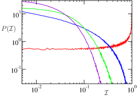
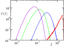
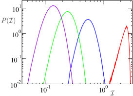
Figure 1: (Color online) Numerically calculated interference distributions on a log-log scale for $x=0.1$ for $n=2,3,4$ (from the left to the right). In each plot, $m=1,2,3,4$ from the right to the left (red, blue, green, purple, respectively). The number of realizations is $n_{r}=10^{6}$ in all cases.

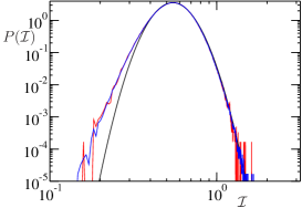
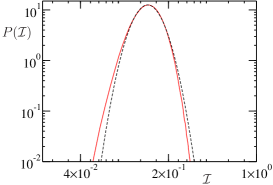
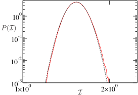
Figure 2: (Color online) Fit of numerically calculated $P({\cal I})$ (red curves) to a log-normal distribution (black dashed curves) at x = 0.1 for (n,m)=(4,2), (4,4) and (8,2) (from left to right). All fits are for $n_{r}=10^{6}$ except for the first plot in which the blue curve is for $n_{r}=10^{7}$.

In the case $n=2$, where the analytical calculation is possible the distributions are very wide (see Arnaud and Braun (2007) for $m=1$ where $P(\mathcal{I})=\frac{1}{2\sqrt{1-\mathcal{I}}}$). For higher values of $n$, the distribution becomes more and more peaked, and, on a log-log scale, more and more symmetric with respect to the maximum. The tails of the distribution decay more rapidly in the non-unitary case. We see that both the most probable value of ${\cal I}$ and the width of the peak decrease when $m$ increases. As expected, the decoherence due to the coupling to the environment destroys the interference more efficiently with increasing $m$. For fixed $m$ the general distribution behaves qualitatively like the distribution for the unitary case studied in Arnaud and Braun (2007), i.e. the most probable interference and mean interference increase with $n$, whereas the width of the distribution decreases with increasing $n$. A change of the temperature essentially shifts the distribution. This is due to a change of the average interference with the temperature as we will see later (see eq.(47)), and justifies why we have plotted all distributions for $x=0.1$.

Fig.2 shows that $P({\cal I})$ is well fitted by a log-normal distribution,

$$P({\cal I})=\frac{\exp\left(\frac{(\log({\cal I})-\mu)^{2}}{2\sigma^{2}}\right)}{{\cal I}\sqrt{2\pi}\sigma}\,.$$ (7)

The fits work particularly well close to the center of the distributions, whereas deviations appear in the wings of the distribution. In addition, the wings appear to be clipped, but this is at least partly an effect of the finite number of realizations available. This is visible from the example $n=4,m=2$, where we have increased the number of realizations $n_{r}$ from $10^{6}$ to $10^{7}$. In the latter case, the clipping appears at substantially larger values of ${\cal I}$.

The numerically obtained distributions suggest that $P(\mathcal{I})$ is for $n>2$ well characterized by its first and second moments. We will now present analytical results for these two moments which confirm the qualitative observations above for arbitrary values of $n$, $m$, and $x$, and make them more quantitative.

II.4 Analytical results

II.4.1 Average interference

The average interference $\langle{\cal I}\rangle$ follows from eq.(II.2),

$$\langle\mathcal{I}\rangle = \frac{1}{Z^{2}}\sum_{\alpha,\gamma\neq\delta}^{n}\sum_{\mu,\nu,\rho,\sigma}^{d}e^{-x\,(\nu+\sigma)}\langle U_{\alpha\mu,\gamma\nu}U_{\alpha\mu,\delta\nu}^{*}U_{\alpha\rho,\gamma\sigma}^{*}U_{\alpha\rho,\delta\sigma}\rangle$$ (8)

where $\langle\,.\rangle\equiv\int dU(.)$ means average over CUE. For the monomials composed of a relatively small number of factors $U_{\alpha\mu,\gamma\nu}$ to be averaged here, the technique of invariant integration is well suited. We use the diagrammatical language introduced in Aubert and Lam (2003, 2004) to express $\langle{\cal I}\rangle$ as

$${\cal I} = \frac{1}{Z^{2}}\sum_{\alpha,\gamma\neq\delta}^{n}\sum_{\mu,\nu,\rho,\sigma}^{d}e^{-x\,(\nu+\sigma)}{\scriptsize\begin{tabular}[]{c}\\ $\alpha\rho$\\ \\ $\alpha\mu$\end{tabular}\begin{tabular}[]{c}\raisebox{-36.98866pt}{\includegraphics[width=59.75095pt]{diag/Fmax.eps}}\end{tabular}\begin{tabular}[]{c}$\delta\sigma$\\ $\gamma\sigma$\\ $\delta\nu$\\ $\gamma\nu$\end{tabular}}$$ (18)

We refer the reader to Aubert and Lam (2003, 2004); Braun (2006) for a detailed explanation and derivation of this technique, but summarize here the main features. For the sake of clarity we revert momentarily to single roman indices $i$, $j$ etc. for rows and columns. All distinct row (column) indices that appear in the matrix elements of the monomial are represented by vertices on the left (right) with the corresponding label, irrespectively of whether or not they arise from a matrix element $U_{ij}$ or its complex conjugate $U_{ij}^{*}$. A complex conjugate factor $U_{ij}^{*}$ is then represented by a thin solid line between the vertices $i$ and $j$, whereas a factor $U_{kl}$ is represented by a dotted line between the vertices $k$ and $l$. When a given matrix element occurs with multiplicity $t$, a single line is drawn with the number $t$ next to it to keep track of the multiplicity. Factors like $|U_{ij}|^{2}$ are represented by thick solid lines, which can also have a multiplicity larger than one. In Aubert and Lam (2003) it was shown that the invariance of the Haar measure under arbitrary unitary transformations leads to the following important properties:

1. The value of a diagram does not depend on the specific values of the vertices. It only depends on the form of the diagram. This means that diagrams can be drawn without specifying the explicit values of the vertices. For example,

   $$\langle U_{11}U_{11}^{*}U_{12}U_{12}^{*}\rangle=\langle U_{24}U_{24}^{*}U_{26}U_{26}^{*}\rangle=\begin{tabular}[]{c}\raisebox{-5.69046pt}{\includegraphics[width=42.67912pt]{diag/F11.eps}}\end{tabular}\,.$$ (19)

2. If for at least one vertex in the diagram, the number of thin solid lines that originates from the vertex differs from the number of dotted lines then the value of the diagram is zero. For example,

   $$\langle U_{11}U_{12}^{*}U_{23}^{*}U_{24}\rangle = \begin{tabular}[]{c}\raisebox{0.0pt}{\includegraphics[width=42.67912pt]{diag/Fmax.eps}}\end{tabular}=0$$ (21)

   $$\langle U_{11}U_{12}^{*}U_{21}U_{22}^{*}\rangle = \begin{tabular}[]{c}\raisebox{-5.69046pt}{\includegraphics[width=42.67912pt]{diag/E2.eps}}\end{tabular}\neq 0\,.$$ (23)

In eq.(18), we sum over all row and column indices and different type of diagrams therefore appear, depending on which vertices coincide. Combinations of indices contribute for which the vertices ($\gamma\nu$) and ($\delta\nu$) collapse on the vertices ($\gamma\sigma$) and ($\delta\sigma$), respectively, i.e. configurations with $\nu=\sigma$. We thus have

$$\langle\mathcal{I}\rangle = \frac{1}{Z^{2}}\sum_{\alpha,\gamma\neq\delta}^{n}\sum_{\mu,\nu,\rho}^{d}e^{-2x\,\nu}{\scriptsize\begin{tabular}[]{c}$\alpha\rho$\\ $\alpha\mu$\end{tabular}\begin{tabular}[]{c}\raisebox{-11.38092pt}{\includegraphics[width=34.14322pt]{diag/E2.eps}}\end{tabular}\begin{tabular}[]{c}$\delta\nu$\\ $\gamma\nu$\end{tabular}}$$ (29)

$$= \frac{1}{Z^{2}}\sum_{\alpha,\gamma\neq\delta}^{n}\Big{(}\sum_{\nu}^{d}e^{-2x\,\nu}\Big{)}\Big{(}\sum_{\mu=\rho}^{d}{\scriptsize\begin{tabular}[]{c}$\alpha\mu$\end{tabular}\begin{tabular}[]{c}\raisebox{-11.38092pt}{\includegraphics[width=34.14322pt]{diag/F11.eps}}\end{tabular}\begin{tabular}[]{c}$\delta\nu$\\ \\ $\gamma\nu$\end{tabular}}+\sum_{\mu\neq\rho}^{d}{\scriptsize\begin{tabular}[]{c}$\alpha\rho$\\ $\alpha\mu$\end{tabular}\begin{tabular}[]{c}\raisebox{-11.38092pt}{\includegraphics[width=34.14322pt]{diag/E2.eps}}\end{tabular}\begin{tabular}[]{c}$\delta\nu$\\ $\gamma\nu$\end{tabular}}\Big{)}\,.$$ (40)

At this point only two types of diagrams remain, and since their values do not depend on the summation indices, we get

$$\langle\mathcal{I}\rangle = \frac{Z(2x)}{Z^{2}(x)}\,n^{2}(n-1)\Big{(}d\begin{tabular}[]{c}\raisebox{-5.69046pt}{\includegraphics[width=42.67912pt]{diag/F11.eps}}\end{tabular}+d(d-1)\begin{tabular}[]{c}\raisebox{-5.69046pt}{\includegraphics[width=42.67912pt]{diag/E2.eps}}\end{tabular}\Big{)}\,.$$ (43)

The values of the two diagrams are easily found Aubert and Lam (2003),

$$= \frac{1}{N(N+1)}$$

$$= \frac{1}{N(N^{2}-1)}\,.$$

The prefactor can be rewritten as

$$h(x)\equiv\frac{Z(2x)}{Z^{2}(x)}=\coth(dx/2)\tanh(x/2),$$ (46)

and we finally obtain, with $d=m$,

$$\langle\mathcal{I}(n,m,x)\rangle=\coth(\frac{mx}{2})\tanh(\frac{x}{2})\frac{nm(n-1)^{2}}{(n^{2}m^{2}-1)}\,.$$ (47)

This is our first central result which we now discuss in detail.

We first observe that the entire temperature dependence is entirely contained in the prefactor $h(x)$. Its limits for $x\to 0$ and $x\to\infty$ are $1/m$ and $1$, respectively. In between, $h(x)$ increases monotonously. We thus find that the average interference decreases with increasing temperature, an intuitively appealing result. Only the dimension of the environment $m=d$ enters the dependence on temperature. This is true in fact for all moments of $P({\cal I})$, as the entire temperature dependence is contained in factors $\exp(-x\nu)$ which are always summed over $\nu=1,\ldots,m$.

In the particular case $m=1$, i.e. $n=N$, we recover as expected the expression for purely unitary propagation Arnaud and Braun (2007),

$$\langle\mathcal{I}(n,1,x)\rangle=\frac{N(N-1)^{2}}{N^{2}-1}=\frac{N(N-1)}{N+1}=\langle\mathcal{I}_{U}(N)\rangle\,.$$ (48)

No entanglement or correlations with the environment can arise in this case, as a single state always factors out, such that the dynamics of ${\cal S}$ remains indeed entirely unitary.

Contrary to what might be expected naively, the unitary result is not recovered for zero temperature, $x\to\infty$. Rather one finds

$$\lim\limits_{x\to\infty}\langle\mathcal{I}(n,m,x)\rangle = \frac{N(n-1)^{2}}{N^{2}-1}\,,$$ (49)

We recall that $N=n\times m$. For $n\gg 1$ and $m$ fixed we have the asymptotic behavior

$$\langle\mathcal{I}_{U}(n)\rangle = n-2+O(\frac{1}{n})$$ (50)

$$\langle\mathcal{I}(n,m,x\to\infty)\rangle = \frac{n-2}{m}+O(\frac{1}{n})\simeq\frac{\langle\mathcal{I}_{U}(n)\rangle}{m}$$ (51)

We see that for $n\gg 1$, the average interference still scales linearly with the system size, but is roughly a factor $m$ smaller than in the unitary case. The reason for this reduction is, of course, that even for a heat bath initially in a pure ground state, the common unitary dynamics of ${\cal S}$ and ${\cal E}$ entangles ${\cal S}$ and ${\cal E}$, such that after tracing out the environment non-unitary evolution of ${\cal S}$ results. The consequent loss of coherence manifests itself in a reduction of interference. In the opposite limit of infinite temperature, $x\to 0$, the temperature dependence of the prefactor $h(x)$ leads to reduction by another factor $m$,

$$\lim\limits_{x\to 0}\langle\mathcal{I}(n,m,x)\rangle = \frac{n(n-1)^{2}}{N^{2}-1}\,.$$ (52)

The additional reduction is also seen in the asymptotic expansion for $n\gg 1$, which reads in this case

$$\langle\mathcal{I}(n,m,x=0)\rangle = \frac{n-2}{m^{2}}+O(\frac{1}{n})\simeq\frac{\langle\mathcal{I}_{U}(n)\rangle}{m^{2}}\,.$$ (53)

For $m\gg 1$ and $n$ fixed we find

$$\langle\mathcal{I}(n,m,x\to\infty)\rangle = \frac{(n-1)^{2}}{nm}+O(\frac{1}{m^{3}})$$ (54)

$$\langle\mathcal{I}(n,m,x=0)\rangle = \frac{(n-1)^{2}}{nm^{2}}+O(\frac{1}{m^{3}})\,.$$ (55)

Eqs.(54) and (55) show that for fixed $n>1$, $\langle\mathcal{I}\rangle$ decreases as $1/m$ ($1/m^{2}$) for zero temperature (infinite temperature). In Fig.3 we plot $\langle\mathcal{I}(n,m,x)\rangle$ for four different temperatures as function of $n$ and $m$. We see that for given temperature, $\langle\mathcal{I}(n,m,x)\rangle$ increases with $n$, but decreases with $m$. For large $n$, with $m$ and $x$ fixed, the increase is essentially proportional to $n$, just as in the unitary case, albeit with a slope reduced by a factor $h(x)/m$. For large $m$, with $n$ and $x$ fixed such that $mx\gg 1$, the decrease of $\langle\mathcal{I}(n,m,x)\rangle$ is roughly as $1/m$ with a prefactor $\frac{(e^{x}-1)^{2}}{e^{2x}-1}\frac{n(n-1)^{2}}{n^{2}}$.

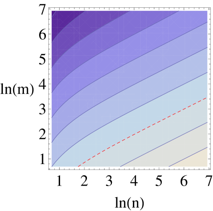
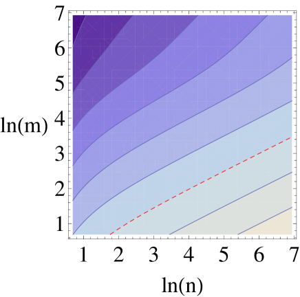
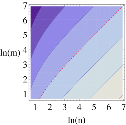
Figure 3: (Color online) Contour plot of $\ln(\langle\mathcal{I}(n,m)\rangle)$ for x=0.001, 0.01, 0.1 and 10 (upper left to lower right), for $n$ and $m$ between 2 and 1024. The distance between the contours is 2, and the red dashed line is for $\ln(\langle\mathcal{I}(n,m)\rangle)=0$. Values increase from dark to bright colors.

More generally, an increase in the dimension of the environment decreases the average interference in a power law fashion with a power that crosses over from $m^{-2}$ for $x=0.001$ to $m^{-1}$ for x=10 and fixed $n$. One should not conclude from this, however, that a quantum system coupled to an infinite dimensional heat bath will never show any quantum interference effect. Rather, it should be kept in mind that we consider here generically strong couplings to the environment, in the sense that a typical joint evolution operator $U$ of ${\cal S}$ and ${\cal E}$ does not distinguish the two subsystems, or, for that matter, a system hamiltonian, bath hamiltonian, and coupling hamiltonian. It is natural that such strong couplings destroy coherence and thus quantum interference rapidly, but the situation can of course be different for weak couplings.

II.4.2 Second moment of the interference distribution

In order to appreciate the width of the interference distribution as function of $m,n$ and $x$, we now calculate the second moment of $P({\cal I})$. By taking the square of the eq.(II.2) we find

$$\mathcal{I}^{2} = \frac{1}{Z^{4}}\sum_{\alpha,\gamma\neq\delta}^{n}\sum_{a,g\neq d}^{n}\sum_{\mu,\rho,p,r}^{d}\sum_{\nu,\sigma,q,s}^{d}e^{-x\,(\nu+\sigma+n+s)}U_{\alpha\mu,\gamma\nu}U_{\alpha\mu,\delta\nu}^{*}U_{\alpha\rho,\gamma\sigma}^{*}U_{\alpha\rho,\delta\sigma}U_{ap,gq}^{*}U_{ap,dq}U_{ar,gs}U_{ar,ds}^{*}$$

The fact that 8 factors $U$ appear now, makes the analytical calculation of $\langle\mathcal{I}^{2}\rangle$ rather cumbersome. As we will see, altogether 19 different diagrams contribute. We give here a rough outline of the derivation, relegating most details and in particular the values of all diagrams to the Appendix. In order to streamline the presentation we introduce the following simplifications of notation:

• First, for the six subsystem indices, we substitute $(\alpha,\gamma,\delta,a,g,d)\to(\alpha_{1},\alpha_{2},\alpha_{3},\alpha_{4},\alpha_{5},\alpha_{6})$.

• Similarly, for the eight environment indices, we replace $(\mu,\rho,p,r,\nu,\sigma,q,s)\to(\mu_{1},\mu_{2},\mu_{3},\mu_{4},\mu_{5},\mu_{6},\mu_{7},\mu_{8})$.

• We then drop the redundant letters $\alpha$ and $\mu$ altogether, both from matrix elements and the diagrams. I.e. we write matrix elements $U_{\alpha_{i}\mu_{j},\alpha_{k}\mu_{l}}$ just as $U_{ij,kl}$. So now $U_{11,11}$ is not the first element of the matrix but it is the element with indices ($\alpha_{1}\mu_{1},\alpha_{1}\mu_{1}$). Recall that all $\alpha$ ($\mu$) indices take values between $1$ and $n$ ($m$), respectively.

• The constraints $\gamma\neq\delta$ and $g\neq d$ read now $\alpha_{2}\neq\alpha_{3}$ and $\alpha_{5}\neq\alpha_{6}$. They are assumed implicitly.

• We also make it a rule that in a sum $\{\alpha_{i},\mu_{j}\}$ denotes the set of all indices which appear explicitly in the summand as indices of matrix elements, or, equivalently, as labels of vertices, with the exception of those which appear under another sum in the same expression. E.g. in $\sum_{\{\alpha_{i},\mu_{j}\}}\sum_{\mu_{5},\mu_{7}}$, the first sum is over all $\alpha$’s and all $\mu$’s that show up in the diagram summed over, with the exception of $\mu_{5}$ and $\mu_{7}$, which are considered separately.

We can then write

$$\langle\mathcal{I}^{2}\rangle = \frac{1}{Z^{4}}\sum_{\{\alpha_{i},\mu_{j}\}}^{(n,m)}e^{-x\,(\mu_{5}+\mu_{6}+\mu_{7}+\mu_{8})}\langle U_{11,35}U_{11,45}^{*}U_{12,36}^{*}U_{12,46}U_{23,57}^{*}U_{23,67}U_{24,58}U_{24,68}^{*}\rangle$$ (56)

$$= \frac{1}{Z^{4}}\sum_{\{\alpha_{i},\mu_{j}\}}^{(n,d)}e^{-x\,(\mu_{5}+\mu_{6}+\mu_{7}+\mu_{8})}{\scriptsize\begin{tabular}[]{c}\\ 2,4\\ \\ 2,3\\ \\ 1,2\\ \\ 1,1\end{tabular}\begin{tabular}[]{c}\raisebox{-22.76228pt}{\includegraphics[width=59.75095pt]{diag/Dmax.eps}}\end{tabular}\begin{tabular}[]{c}6,8\\ 5,8\\ 6,7\\ 5,7\\ 4,6\\ 3,6\\ 4,5\\ 3,5\end{tabular}}\,.$$ (74)

We re-emphasize that the indices of $U$ which appear in eq.(56) are indices of indices, e.g. $U_{11,35}\equiv U_{\alpha_{1}\mu_{1},\alpha_{3}\mu_{5}}$. As for equation (8), the only non–vanishing contributions arise from diagrams without open ends. They correspond to three distinct configurations of the summation indices, namely $\mu_{5}=\mu_{6}\textrm{ and }\mu_{7}=\mu_{8}$, or $\alpha_{3}=\alpha_{5},\alpha_{4}=\alpha_{6},\mu_{5}=\mu_{7}\textrm{, and }\mu_{6}=\mu_{8}$, or $\alpha_{3}=\alpha_{6},\alpha_{4}=\alpha_{5},\mu_{5}=\mu_{8}\textrm{, and }\mu_{6}=\mu_{7}$. These three configurations give rise to three sums,

$$\langle\mathcal{I}^{2}\rangle = \frac{1}{Z^{4}}\Big{(}\sum_{\{\alpha_{i},\mu_{j}\}}^{(n,m)}\sum_{\mu_{5},\mu_{7}}^{m}e^{-2x\,(\mu_{5}+\mu_{7})}{\scriptsize\begin{tabular}[]{c}2,4\\ 2,3\\ 1,2\\ 1,1\end{tabular}\begin{tabular}[]{c}\raisebox{-36.98866pt}{\includegraphics[width=36.98866pt]{diag/D44.eps}}\end{tabular}\begin{tabular}[]{c}6,7\\ 5,7\\ 4,5\\ 3,5\end{tabular}}+\sum_{\{\alpha_{i},\mu_{j}\}}^{(n,m)}\sum_{\alpha_{3},\alpha_{4}}^{n}\sum_{\mu_{5}\neq\mu_{6}}^{m}e^{-2x\,(\mu_{5}+\mu_{6})}{\scriptsize\begin{tabular}[]{c}2,4\\ 1,2\\ 2,3\\ 1,1\end{tabular}\begin{tabular}[]{c}\raisebox{-36.98866pt}{\includegraphics[width=36.98866pt]{diag/D44.eps}}\end{tabular}\begin{tabular}[]{c}4,6\\ 3,6\\ 4,5\\ 3,5\end{tabular}}$$ (103)

$$+\sum_{\{\alpha_{i},\mu_{j}\}}^{(n,m)}\sum_{\alpha_{3},\alpha_{4}}^{n}\sum_{\mu_{5}\neq\mu_{6}}^{m}e^{-2x\,(\mu_{5}+\mu_{6})}{\scriptsize\begin{tabular}[]{c}2,3\\ 1,2\\ 2,4\\ 1,1\end{tabular}\begin{tabular}[]{c}\raisebox{-36.98866pt}{\includegraphics[width=36.98866pt]{diag/D44.eps}}\end{tabular}\begin{tabular}[]{c}4,6\\ 3,6\\ 4,5\\ 3,5\end{tabular}}\Big{)}\,.$$

The last two terms are equal as can be seen by exchanging the summation indices $\alpha_{3}\leftrightarrow\alpha_{4}$. We are therefore left with

$$\langle\mathcal{I}^{2}\rangle = \frac{1}{Z^{4}}\Big{(}\sum_{\{\alpha_{i},\mu_{j}\}}^{(n,m)}\sum_{\mu_{5}\mu_{7}}^{m}e^{-2x\,(\mu_{5}+\mu_{7})}{\scriptsize\begin{tabular}[]{c}2,4\\ 2,3\\ 1,2\\ 1,1\end{tabular}\begin{tabular}[]{c}\raisebox{-36.98866pt}{\includegraphics[width=36.98866pt]{diag/D44.eps}}\end{tabular}\begin{tabular}[]{c}6,7\\ 5,7\\ 4,5\\ 3,5\end{tabular}}+2\sum_{\{\alpha_{i},\mu_{j}\}}^{(n,m)}\sum_{\alpha_{3}\alpha_{4}}^{n}\sum_{\mu_{5}\neq\mu_{6}}^{m}e^{-2x\,(\mu_{5}+\mu_{6})}{\scriptsize\begin{tabular}[]{c}2,4\\ 1,2\\ 2,3\\ 1,1\end{tabular}\begin{tabular}[]{c}\raisebox{-36.98866pt}{\includegraphics[width=36.98866pt]{diag/D44.eps}}\end{tabular}\begin{tabular}[]{c}4,6\\ 3,6\\ 4,5\\ 3,5\end{tabular}}\Big{)}$$ (122)

$$\equiv \frac{1}{Z^{4}}(A+2B)\,.$$ (123)

The terms $A$ and $B$ depend on 19 different diagrams which we calculate again by invariant integration. For $A$ we have

$$A = \sum_{\{\alpha_{i},\mu_{j}\}}^{(n,m)}\sum_{\mu_{5},\mu_{7}}^{m}e^{-2x\,(\mu_{5}+\mu_{7})}{\scriptsize\begin{tabular}[]{c}2,4\\ 2,3\\ 1,2\\ 1,1\end{tabular}\begin{tabular}[]{c}\raisebox{-36.98866pt}{\includegraphics[width=36.98866pt]{diag/D44.eps}}\end{tabular}\begin{tabular}[]{c}6,7\\ 5,7\\ 4,5\\ 3,5\end{tabular}}$$ (133)

$$= \sum_{\{\alpha_{i},\mu_{j}\}}^{(n,m)}\Big{(}\sum_{\mu_{5}=\mu_{7}}^{m}e^{-4x\,\mu_{5}}{\scriptsize\begin{tabular}[]{c}2,4\\ 2,3\\ 1,2\\ 1,1\end{tabular}\begin{tabular}[]{c}\raisebox{-36.98866pt}{\includegraphics[width=36.98866pt]{diag/D44.eps}}\end{tabular}\begin{tabular}[]{c}6,5\\ 5,5\\ 4,5\\ 3,5\end{tabular}}+\sum_{\mu_{5}\neq\mu_{7}}^{m}e^{-2x\,(\mu_{5}+\mu_{7})}{\scriptsize\begin{tabular}[]{c}2,4\\ 2,3\\ 1,2\\ 1,1\end{tabular}\begin{tabular}[]{c}\raisebox{-36.98866pt}{\includegraphics[width=36.98866pt]{diag/D44.eps}}\end{tabular}\begin{tabular}[]{c}6,7\\ 5,7\\ 4,5\\ 3,5\end{tabular}}\Big{)}$$ (152)

$$= \sum_{\{\alpha_{i},\mu_{j}\}}^{(n,m)}\Big{(}{\scriptsize\begin{tabular}[]{c}2,4\\ 2,3\\ 1,2\\ 1,1\end{tabular}\begin{tabular}[]{c}\raisebox{-36.98866pt}{\includegraphics[width=36.98866pt]{diag/D44.eps}}\end{tabular}\begin{tabular}[]{c}6\\ 5\\ 4\\ 3\end{tabular}}(\sum_{\mu_{5}=\mu_{7}}^{m}e^{-4x\,\mu_{5}})+{\scriptsize\begin{tabular}[]{c}2,4\\ 2,3\\ 1,2\\ 1,1\end{tabular}\begin{tabular}[]{c}\raisebox{-36.98866pt}{\includegraphics[width=36.98866pt]{diag/D44.eps}}\end{tabular}\begin{tabular}[]{c}$\bar{6}$\\ $\bar{5}$\\ 4\\ 3\end{tabular}}(\sum_{\mu_{5}\neq\mu_{7}}^{m}e^{-2x\,(\mu_{5}+\mu_{7})})\Big{)}$$ (171)

$$= \sum_{\{\alpha_{i},\mu_{j}\}}^{(n,m)}\Big{(}f(x){\scriptsize\begin{tabular}[]{c}2,4\\ 2,3\\ 1,2\\ 1,1\end{tabular}\begin{tabular}[]{c}\raisebox{-36.98866pt}{\includegraphics[width=36.98866pt]{diag/D44.eps}}\end{tabular}\begin{tabular}[]{c}6\\ 5\\ 4\\ 3\end{tabular}}+g(x){\scriptsize\begin{tabular}[]{c}2,4\\ 2,3\\ 1,2\\ 1,1\end{tabular}\begin{tabular}[]{c}\raisebox{-36.98866pt}{\includegraphics[width=36.98866pt]{diag/D44.eps}}\end{tabular}\begin{tabular}[]{c}$\bar{6}$\\ $\bar{5}$\\ 4\\ 3\end{tabular}}\Big{)}\,.$$ (190)

The single indices on the right hand sides of the diagrams in (171) now decode only $\alpha$’s; $\mu_{1}\ldots\mu_{4}$ still appear explicitly on the left column of vertices, $\mu_{6}$ and $\mu_{8}$ were chosen identical to $\mu_{5}$ and $\mu_{7}$, respectively, and the latter two indices are still summed over. A ”bar” vertex is a vertex which cannot collapse with a ”normal” vertex even if both values of the corresponding $\alpha$’s (or $\mu$’s) are the same. The vertices labeled $\bar{5}$ and $\bar{6}$ (which stand here for $\alpha_{5}$ and $\alpha_{6}$) inherit this property from the $\mu_{7}$ part still present in (152): The restriction $\mu_{5}\neq\mu_{7}$ implies indeed that none of the two top vertices can collapse with either of the two bottom vertices in the second diagram. Thus ”normal” and ”bar” vertices can only collapse on vertices of the same kind. The constraint $\alpha_{5}\neq\alpha_{6}$ is still implicit. The functions $f(x)$ et $g(x)$ are defined as

$$f(x) = \left(\frac{1-e^{-4x\,d}}{e^{4x\,}-1}\right)=Z(4x)$$ (191)

$$g(x) = e^{-6x\,}\left(\frac{1-e^{-2x\,d}}{1-e^{-2x\,}}\right)\left(\frac{1-e^{-2x\,(d-1)}}{1-e^{-4x\,}}\right)=Z^{2}(2x)-Z(4x)\,.$$ (192)

With this, we have introduced all notational innovations which allow the analytical calculation of $\langle\mathcal{I}^{2}\rangle$. The rest of the calculations amounts to identifying all possible non-zero configurations of collapsing vertices allowed by the remaining summation variables. The explicit expansion of the terms $A$ and $B$ finally leads to

$$\langle\mathcal{I}^{2}\rangle=\frac{n}{Z^{4}}\Big{[}f(x)\Big{(}A_{1}+(n-1)A_{3}\Big{)}+g(x)\Big{(}A_{2}+(n-1)A_{4}+n(n-1)B_{1}+n(n-1)^{2}B_{2}\Big{)}\Big{]}.$$ (193)

Here, the parameter $d$ in the functions $f$ and $g$ is $d=m$. The terms $A_{i}$ and $B_{i}$ are defined and calculated explicitly in the Appendix. They only depend on $n$ and $m$.

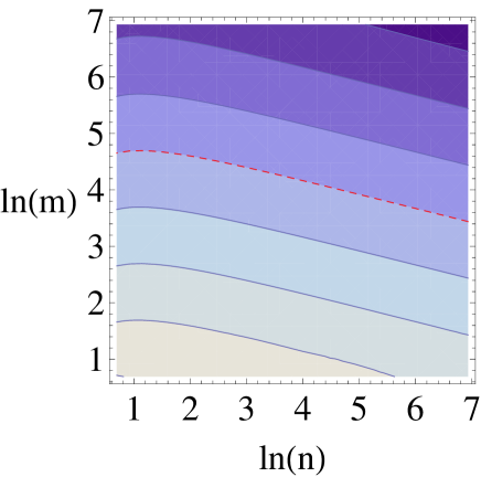
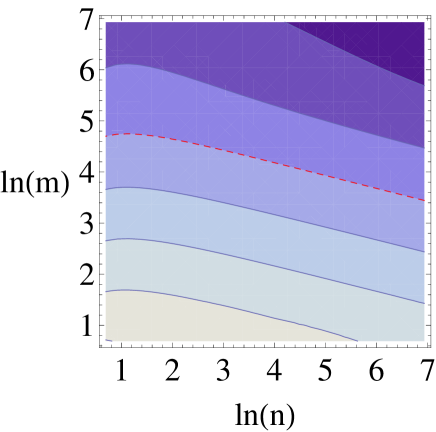
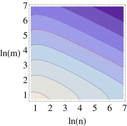
Figure 4: (Color online) Contour plot of $\ln(\sigma_{\mathcal{I}}(n,m))$ for x=0.001, 0.01, 0.1 and 10 (upper left to lower right), for $n$ and $m$ between 2 and 1024. The distance between the contours is 2 and the dashed line is for $\ln(\langle\mathcal{I}(n,m)\rangle)=-10$, except for the last plot where the distance is 1 and the dashed line is for $\ln(\sigma_{\mathcal{I}}(n,m))=-6$. Values increase from dark to bright colors.

In Fig.4 we plot the standard deviation of the distribution of $\mathcal{I}$, $\sigma_{\mathcal{I}}(n,m,x)=(\langle\mathcal{I}^{2}\rangle-\langle\mathcal{I}\rangle^{2})^{1/2}$ for four different temperatures as function of $n$ and $m$. For given temperature, $\sigma_{\mathcal{I}}(n,m,x)$ decreases with $n$ and $m$. The log-log-log plot shows that the decay behaves as a power law in $n$ and in $m$. The corresponding powers can be found from an asymptotic expansion of the variance $var(n,m,x)=\sigma_{\mathcal{I}}^{2}(n,m,x)$ for $n\gg 1$ or for $m\gg 1$ in the limits of zero or infinite temperature. For fixed $m$, we find for $n\gg 1$

$$var(n,m,x\to\infty) = \frac{2(m-1)^{2}}{nm^{4}}-\frac{4(m^{4}-3m^{3}+3m^{2}-5m+3)}{m^{6}n^{2}}+O(\frac{1}{n^{3}})$$ (194)

$$var(n,m,x=0) = \frac{2(m^{2}-1)}{nm^{6}}+\frac{8-4m^{4}}{m^{8}n^{2}}+O(\frac{1}{n^{3}})\,.$$ (195)

This should be compared to the unitary case, where the asymptotic expansion reads $var_{U}(n)=\frac{4}{n^{2}}+O(\frac{1}{n^{3}})$, as is still evident from eqs.(194) and (195) by choosing $m=1$. We see that the variance decays more slowly as function of $n$ in the presence of decoherence, i.e. as $1/n$ instead of as $1/n^{2}$ in the unitary case. In other words, decoherence tends to slow down convergence of the interference distribution to a narrow peak. Nevertheless, the power law decay of the variance as function of $n$ implies that, also in the non-unitary case, the interference distribution becomes for $n\gg 1$ a very narrow peak centered about the average value (which itself increases with $n$, see eqs.(49) and (52)).

Asymptotic expansion of $var(n,m,x)$ as function of $m\gg 1$ with fixed $n$ gives

$$var(n,m,x\to\infty) = \frac{2(n-1)^{2}}{n^{3}m^{2}}+O(\frac{1}{m^{3}})$$ (196)

$$var(n,m,x=0) = \frac{(n-1)^{2}}{n^{3}m^{4}}+O(\frac{1}{m^{6}})\,.$$ (197)

Thus, also an increase of the dimension of the environmental Hilbert space narrows the interference distribution. However, since according to (54,55), the average interference decays as $1/m$ ($1/m^{2}$) for $x\to\infty$ ($x\to 0$), the relative width, i.e. standard deviation divided by the average value, is asymptotically independent of the dimension of the environment.

In the case $m=d=1$ ($n=N$) all the prefactors $m[i]$ (see Appendix) are zero if $i\geq 1$. With the same parameters we have furthermore from eqs.(191,192), $f(x)=Z=1$, and $g(x)=0$. Thus the expression (193) of $\langle\mathcal{I}^{2}\rangle$ simplifies considerably,

$$\langle\mathcal{I}^{2}\rangle = \Big{(}NA_{1}+N(N-1)A_{3}\Big{)}$$

$$= \Big{(}N\big{(}N[3]\begin{tabular}[]{c}\includegraphics[width=28.45274pt]{diag/D14.eps}\end{tabular}+4N[2]\begin{tabular}[]{c}\includegraphics[width=28.45274pt]{diag/D13.eps}\end{tabular}+2N[1]\begin{tabular}[]{c}\includegraphics[width=28.45274pt]{diag/D12.eps}\end{tabular}\big{)}$$

$$+N(N-1)\big{(}N[3]\begin{tabular}[]{c}\includegraphics[width=28.45274pt]{diag/Da24.eps}\end{tabular}+4N[2]\begin{tabular}[]{c}\includegraphics[width=28.45274pt]{diag/Da23.eps}\end{tabular}+2N[1]\begin{tabular}[]{c}\includegraphics[width=28.45274pt]{diag/Da22.eps}\end{tabular}\big{)}\Big{)}$$

$$= \frac{N\left(N^{3}-5N+8\right)-4}{(N+1)(N+3)}\,.$$

As expected this leads to the standard deviation $\sigma_{\mathcal{I}}=\frac{2}{N+1}\sqrt{\frac{N-1}{N+3}}$, identical to the expression for purely unitary propagation Arnaud and Braun (2007).

The numerical results in section II.3 are in very good agreement with our analytical results, as can be seen in table 1 where we compare the numerically obtained average values and standard deviations for the examples shown in fig.2 and for $(n,m)=(4,8)$ and (8,4) to the corresponding analytical results.

n	m	$\langle{\cal I}\rangle$ (num.)	$\langle{\cal I}\rangle$ (ana.)	$\sigma_{\cal I}$ (num.)	$\sigma_{\cal I}$ (ana.)
4	2	0.57279	0.57286	0.11728	0.11719
4	4	0.14296	0.14293	0.03260	0.03255
4	8	0.03702	0.03702	0.00864	0.00864
8	2	1.54120	1.54109	0.09022	0.09409
8	4	0.38796	0.38796	0.02670	0.02666

Table 1: Comparison of numerical and analytical values of $\langle{\cal I}\rangle$ and $\sigma_{\cal I}$. All results are rounded to five digits after the decimal point.

III Interference for a spin coupled to several spins

In this part, we generalize the previous calculations to a situation where the environment consists of $s$ independent spins with $d$ energy levels with energy spacing $\hbar\Omega$. Thus, the dimension of the environment is $m=d^{s}$. The hamiltonian of this system reads

$$H^{(s)}=\sum_{k=1}^{s}H_{k}^{(1)}\,,$$ (200)

where $H_{k}^{(1)}$ is the hamiltonian of spin number $k$ (eq.(3)). The components of $H^{(s)}$ in its eigenbasis are

$$H^{(s)}_{\nu\rho} = \hbar\Omega\left(\sum_{k=1}^{s}\nu_{k}\right)\delta_{\nu\rho}$$ (201)

with the notation for the indices $\nu=(\nu_{1},\nu_{2},...,\nu_{s})$ and $\rho=(\rho_{1},\rho_{2},...,\rho_{s})$

The density matrix corresponding to the thermal state of such a system factorizes, $\epsilon^{(s)}=\epsilon^{(s)}=\epsilon^{(1)\otimes s},$ which leads to the components

$$\epsilon^{(s)}_{\nu\rho} = \frac{e^{-x\,S(\nu)}\delta_{\nu\rho}}{Z^{s}}$$ (202)

with $x=\beta\hbar\Omega$, $S(\nu)=\sum_{k=1}^{s}\nu_{k}$, and where $Z$ is the partition function of the thermal state of a single spin introduced in the previous section. It turns out that in order to generalize the previous calculation of $<\mathcal{I}>$ and $<\mathcal{I}^{2}>$ to this kind of environment, we just have to replace $Z$ by $Z^{s}$ in eqs.(43), (191), and (192), and keep $d=m^{s}$ instead of $d=m$. This is again a consequence of the fact that the values of the diagrams do not depend on the indices of the vertices. Thus, the same values are obtained even for composite indices reflecting several subsystems, and only the multiplicities and temperature dependent factors are modified. Since the spins of the heat bath are taken as non-interacting, the sums over the thermal factors just gives rise to powers of the single spin thermal factors, as is the case also for the calculation of the partition function for $s$ spins. This means that we have to replace

$$f(x) \rightarrow \sum_{\mu}e^{-4xS(\mu)}=\sum_{\mu_{1}}^{d}...\sum_{\mu_{s}}^{d}e^{-4x\mu_{1}}...e^{-4x\mu_{s}}=Z^{s}(4x)=f^{s}(x)$$

$$g(x) \rightarrow \sum_{\mu\neq\nu}e^{-2x(S(\mu)+S(\nu))}=\sum_{\mu,\nu}e^{-2x(S(\mu)+S(\nu))}-\sum_{\mu}e^{-4xS(\mu)}=Z^{s}(2x)-Z^{s}(4x)\,.$$

The expressions for $\langle\mathcal{I}\rangle$ and $\langle\mathcal{I}^{2}\rangle$ become

$$\langle\mathcal{I}\rangle = n^{2}(n-1)h^{s}(x)\Big{(}d\begin{tabular}[]{c}\raisebox{-5.69046pt}{\includegraphics[width=42.67912pt]{diag/F11.eps}}\end{tabular}+d(d-1)\begin{tabular}[]{c}\raisebox{-5.69046pt}{\includegraphics[width=42.67912pt]{diag/E2.eps}}\end{tabular}\Big{)}$$ (205)

$$= \Big{(}\coth(\frac{dx}{2})\tanh(\frac{x}{2})\Big{)}^{s}\Big{(}\frac{nd^{s}(n-1)^{2}}{n^{2}d^{2s}-1}\Big{)}\,,$$ (206)

$$\langle\mathcal{I}^{2}\rangle = \frac{n}{Z^{4s}}\Big{[}f^{s}(x)\Big{(}A_{1}+(n-1)A_{3}\Big{)}$$ (207)

$$+g^{s}(x)\Big{(}A_{2}+(n-1)A_{4}+n(n-1)B_{1}+n(n-1)^{2}B_{2}\Big{)}\Big{]}\,.$$

The argument $m$ in the terms $A_{i}$ and $B_{i}$ in eqs.(205,207) is now $m=d^{s}$. It means that $s$ spins of size $(d-1)/2$ act very similarly as a single spin of size $(d^{s}-1)/2$, when it comes to their influence on the first and second moments of $P({\cal I})$. The only difference lies in the temperature dependent prefactors $f(x),g(x)$ and $h(x)$. For a single spin of size $(d^{s}-1)/2$, $d$ in eqs.(46,191,192) is given by the dimension of the environment $m=d^{s}$, but in eqs.(205,207) we have $s=1$ for a single spin. For $s$ spins of size $(d-1)/2$ the dimension $d$ in eqs.(46,191,192) remains, and $s$ is the number of spins in eqs. (205,207). In the limits $x\to 0$ or $x\to\infty$ the expressions coincide for the two situations.

IV Summary

We have investigated quantitatively how quantum interference is affected by decoherence. Based on a distribution of unitary matrices drawn from CUE which describe the joint propagation of system and heat bath, we have shown that the average interference increases roughly linearly with the Hilbert space dimension $n$ of the system, but decays as a power of the dimension $m$ of the environment. That power depends on the temperature of the environment (chosen here as one or several non-interacting spins), with a decay that essentially scales like $1/m^{2}$ for $T=0$, and as $1/m^{3}$ for $T\to\infty$. The width of the distribution decreases more slowly when decoherence becomes important, but for fixed $m$, the width of the distribution still decays as $1/\sqrt{n}$ (instead of as $1/n$ in the unitary case). Thus, for $n\gg 1$ and $m$ fixed, the distribution of quantum interference is still a sharp peak concentrated on the average value. Numerically we have shown that the interference distribution in the non-unitary case can be well fitted to a log-normal distribution for sufficiently large $n$, which implies that the number of i-bits Braun and Georgeot (2006) is to good approximation Gaussian distributed.

Acknowledgments: We would like to thank CALMIP (Toulouse) for the use of their computers. This work was supported by the Agence National de la Recherche (ANR), project INFOSYSQQ.

V Appendix

We provide here the remaining details of the calculation of the terms $A$ and $B$ in the expression for $\langle\mathcal{I}^{2}\rangle$, eq.(123), as well as the values of the resulting diagrams.

V.1 The $A$ term

¿From eq.(190) we have

$$A = \sum_{\{\alpha_{i},\mu_{j}\}}^{(n,m)}\Big{(}\sum_{\{\alpha_{1}=\alpha_{2}\}}^{n}f(x){\scriptsize\begin{tabular}[]{c}1,4\\ 1,3\\ 1,2\\ 1,1\end{tabular}\begin{tabular}[]{c}\raisebox{-36.98866pt}{\includegraphics[width=36.98866pt]{diag/D44.eps}}\end{tabular}\begin{tabular}[]{c}6\\ 5\\ 4\\ 3\end{tabular}}+g(x){\scriptsize\begin{tabular}[]{c}1,4\\ 1,3\\ 1,2\\ 1,1\end{tabular}\begin{tabular}[]{c}\raisebox{-36.98866pt}{\includegraphics[width=36.98866pt]{diag/D44.eps}}\end{tabular}\begin{tabular}[]{c}$\bar{6}$\\ $\bar{5}$\\ 4\\ 3\end{tabular}}$$ (245)

$$+\sum_{\{\alpha_{1}\neq\alpha_{2}\}}^{n}f(x){\scriptsize\begin{tabular}[]{c}2,4\\ 2,3\\ 1,2\\ 1,1\end{tabular}\begin{tabular}[]{c}\raisebox{-36.98866pt}{\includegraphics[width=36.98866pt]{diag/D44.eps}}\end{tabular}\begin{tabular}[]{c}6\\ 5\\ 4\\ 3\end{tabular}}+g(x){\scriptsize\begin{tabular}[]{c}2,4\\ 2,3\\ 1,2\\ 1,1\end{tabular}\begin{tabular}[]{c}\raisebox{-36.98866pt}{\includegraphics[width=36.98866pt]{diag/D44.eps}}\end{tabular}\begin{tabular}[]{c}$\bar{6}$\\ $\bar{5}$\\ 4\\ 3\end{tabular}}\Big{)}$$

$$= \sum_{\{\alpha_{i},\mu_{j}\}}^{(n,m)}\Big{(}n\,f(x){\scriptsize\begin{tabular}[]{c}4\\ 3\\ 2\\ 1\end{tabular}\begin{tabular}[]{c}\raisebox{-36.98866pt}{\includegraphics[width=36.98866pt]{diag/D44.eps}}\end{tabular}\begin{tabular}[]{c}6\\ 5\\ 4\\ 3\end{tabular}}+n\,g(x){\scriptsize\begin{tabular}[]{c}4\\ 3\\ 2\\ 1\end{tabular}\begin{tabular}[]{c}\raisebox{-36.98866pt}{\includegraphics[width=36.98866pt]{diag/D44.eps}}\end{tabular}\begin{tabular}[]{c}$\bar{6}$\\ $\bar{5}$\\ 4\\ 3\end{tabular}}$$ (283)

$$+n(n-1)\,f(x){\scriptsize\begin{tabular}[]{c}$\bar{4}$\\ $\bar{3}$\\ 2\\ 1\end{tabular}\begin{tabular}[]{c}\raisebox{-36.98866pt}{\includegraphics[width=36.98866pt]{diag/D44.eps}}\end{tabular}\begin{tabular}[]{c}6\\ 5\\ 4\\ 3\end{tabular}}+n(n-1)\,g(x){\scriptsize\begin{tabular}[]{c}$\bar{4}$\\ $\bar{3}$\\ 2\\ 1\end{tabular}\begin{tabular}[]{c}\raisebox{-36.98866pt}{\includegraphics[width=36.98866pt]{diag/D44.eps}}\end{tabular}\begin{tabular}[]{c}$\bar{6}$\\ $\bar{5}$\\ 4\\ 3\end{tabular}}\Big{)}$$

$$= n\,f(x)A_{1}+n\,g(x)A_{2}+n(n-1)\,f(x)A_{3}+n(n-1)\,g(x)A_{4}\,.$$ (284)

By taking into account the constraints on the $\alpha_{i}$ we get

$$A_{1} = \sum_{\{\alpha_{i},\mu_{j}\}}^{(n,m)}{\scriptsize\begin{tabular}[]{c}4\\ 3\\ 2\\ 1\end{tabular}\begin{tabular}[]{c}\raisebox{-36.98866pt}{\includegraphics[width=36.98866pt]{diag/D44.eps}}\end{tabular}\begin{tabular}[]{c}6\\ 5\\ 4\\ 3\end{tabular}}$$

$$= \sum_{\{\mu_{j}\}}^{m}\left(n[3]{\scriptsize\begin{tabular}[]{c}4\\ 3\\ 2\\ 1\end{tabular}\begin{tabular}[]{c}\raisebox{-36.98866pt}{\includegraphics[width=36.98866pt]{diag/D44.eps}}\end{tabular}\begin{tabular}[]{c}\\ \\ \\ \end{tabular}}+4n[2]{\scriptsize\begin{tabular}[]{c}4\\ 3\\ 2\\ 1\end{tabular}\begin{tabular}[]{c}\includegraphics[width=28.45274pt]{diag/D43.eps}\end{tabular}\begin{tabular}[]{c}\\ \\ \end{tabular}}+2n[1]{\scriptsize\begin{tabular}[]{c}4\\ 3\\ 2\\ 1\end{tabular}\begin{tabular}[]{c}\includegraphics[width=28.45274pt]{diag/D42.eps}\end{tabular}\begin{tabular}[]{c}\\ \end{tabular}}\right)$$

$$= n[3]A_{11}+4n[2]A_{12}+2n[1]A_{13}\,,$$

with $n[i]=n(n-1)(n-2)...(n-i)$. We check that we have the $n[3]+4n[2]+2n[1]=n^{2}(n-1)^{2}$ configurations corresponding to the sum over the four indices $\alpha_{j}$ with the two constrains $\alpha_{3}\neq\alpha_{4}$ and $\alpha_{5}\neq\alpha_{6}$. The $A_{1k}$ read

$$A_{11} = \sum_{\{\mu_{j}\}}^{m}{\scriptsize\begin{tabular}[]{c}4\\ 3\\ 2\\ 1\end{tabular}\begin{tabular}[]{c}\raisebox{-36.98866pt}{\includegraphics[width=36.98866pt]{diag/D44.eps}}\end{tabular}\begin{tabular}[]{c}\\ \\ \\ \end{tabular}}$$

$$= m[3]\begin{tabular}[]{c}\includegraphics[width=28.45274pt]{diag/D44.eps}\end{tabular}+m[2]\Big{(}4\begin{tabular}[]{c}\includegraphics[width=28.45274pt]{diag/Da34.eps}\end{tabular}+2\begin{tabular}[]{c}\includegraphics[width=28.45274pt]{diag/Db34.eps}\end{tabular}\Big{)}$$

$$+m[1]\Big{(}2\begin{tabular}[]{c}\includegraphics[width=28.45274pt]{diag/Dc24.eps}\end{tabular}+\begin{tabular}[]{c}\includegraphics[width=28.45274pt]{diag/Da24.eps}\end{tabular}+4\begin{tabular}[]{c}\includegraphics[width=28.45274pt]{diag/Db24.eps}\end{tabular}\big{)}+m\begin{tabular}[]{c}\includegraphics[width=28.45274pt]{diag/D14.eps}\end{tabular},$$

$$A_{12} = \sum_{\{\mu_{j}\}}^{m}{\scriptsize\begin{tabular}[]{c}4\\ 3\\ 2\\ 1\end{tabular}\begin{tabular}[]{c}\includegraphics[width=28.45274pt]{diag/D43.eps}\end{tabular}\begin{tabular}[]{c}\\ \\ \end{tabular}}$$

$$= m[3]\begin{tabular}[]{c}\includegraphics[width=28.45274pt]{diag/D43.eps}\end{tabular}+2m[2]\Big{(}\begin{tabular}[]{c}\includegraphics[width=28.45274pt]{diag/Db33.eps}\end{tabular}+\begin{tabular}[]{c}\includegraphics[width=28.45274pt]{diag/Dc33.eps}\end{tabular}+\begin{tabular}[]{c}\includegraphics[width=28.45274pt]{diag/Da33.eps}\end{tabular}\Big{)}$$

$$+m[1]\Big{(}\begin{tabular}[]{c}\includegraphics[width=28.45274pt]{diag/Da23.eps}\end{tabular}+\begin{tabular}[]{c}\includegraphics[width=28.45274pt]{diag/Dd23.eps}\end{tabular}+\begin{tabular}[]{c}\includegraphics[width=28.45274pt]{diag/Dc23.eps}\end{tabular}\Big{)}+4m[1]\begin{tabular}[]{c}\includegraphics[width=28.45274pt]{diag/Db23.eps}\end{tabular}+m\begin{tabular}[]{c}\includegraphics[width=28.45274pt]{diag/D13.eps}\end{tabular},$$

$$A_{13} = \sum_{\{\mu_{j}\}}^{m}{\scriptsize\begin{tabular}[]{c}4\\ 3\\ 2\\ 1\end{tabular}\begin{tabular}[]{c}\includegraphics[width=28.45274pt]{diag/D42.eps}\end{tabular}\begin{tabular}[]{c}\\ \end{tabular}}$$

$$= m[3]\begin{tabular}[]{c}\includegraphics[width=28.45274pt]{diag/D42.eps}\end{tabular}+m[2]\Big{(}4\begin{tabular}[]{c}\includegraphics[width=28.45274pt]{diag/Da32.eps}\end{tabular}+2\begin{tabular}[]{c}\includegraphics[width=28.45274pt]{diag/Db32.eps}\end{tabular}\Big{)}$$

$$+m[1]\Big{(}2\begin{tabular}[]{c}\includegraphics[width=28.45274pt]{diag/Da22.eps}\end{tabular}+\begin{tabular}[]{c}\includegraphics[width=28.45274pt]{diag/Db22.eps}\end{tabular}+4\begin{tabular}[]{c}\includegraphics[width=28.45274pt]{diag/Dc22.eps}\end{tabular}\Big{)}+m\begin{tabular}[]{c}\includegraphics[width=28.45274pt]{diag/D12.eps}\end{tabular}\,.$$

For $A_{2}$ we obtain directly

$$A_{2} = \sum_{\{\alpha_{i},\mu_{j}\}}^{(n,m)}{\scriptsize\begin{tabular}[]{c}4\\ 3\\ 2\\ 1\end{tabular}\begin{tabular}[]{c}\raisebox{-36.98866pt}{\includegraphics[width=36.98866pt]{diag/D44.eps}}\end{tabular}\begin{tabular}[]{c}$\bar{6}$\\ $\bar{5}$\\ 4\\ 3\end{tabular}}=n^{2}(n-1)^{2}A_{11}\,,$$

whereas $A_{3}$ is given by

$$A_{3} = \sum_{\{\alpha_{i},\mu_{j}\}}^{(n,m)}{\scriptsize\begin{tabular}[]{c}$\bar{4}$\\ $\bar{3}$\\ 2\\ 1\end{tabular}\begin{tabular}[]{c}\raisebox{-36.98866pt}{\includegraphics[width=36.98866pt]{diag/D44.eps}}\end{tabular}\begin{tabular}[]{c}6\\ 5\\ 4\\ 3\end{tabular}}$$

$$= \sum_{\{\mu_{j}\}}^{m}\left(n[3]{\scriptsize\begin{tabular}[]{c}$\bar{4}$\\ $\bar{3}$\\ 2\\ 1\end{tabular}\begin{tabular}[]{c}\raisebox{-36.98866pt}{\includegraphics[width=36.98866pt]{diag/D44.eps}}\end{tabular}\begin{tabular}[]{c}\\ \\ \\ \end{tabular}}+4n[2]{\scriptsize\begin{tabular}[]{c}$\bar{4}$\\ $\bar{3}$\\ 2\\ 1\end{tabular}\begin{tabular}[]{c}\includegraphics[width=28.45274pt]{diag/D43.eps}\end{tabular}\begin{tabular}[]{c}\\ \\ \end{tabular}}+2n[1]{\scriptsize\begin{tabular}[]{c}$\bar{4}$\\ $\bar{3}$\\ 2\\ 1\end{tabular}\begin{tabular}[]{c}\includegraphics[width=28.45274pt]{diag/D42.eps}\end{tabular}\begin{tabular}[]{c}\\ \end{tabular}}\right)$$

$$= n[3]A_{31}+4n[2]A_{32}+2n[1]A_{33}\,.$$

The $A_{3k}$ are

$$A_{31} = \sum_{\{\mu_{j}\}}^{m}{\scriptsize\begin{tabular}[]{c}$\bar{4}$\\ $\bar{3}$\\ 2\\ 1\end{tabular}\begin{tabular}[]{c}\raisebox{-36.98866pt}{\includegraphics[width=36.98866pt]{diag/D44.eps}}\end{tabular}\begin{tabular}[]{c}\\ \\ \\ \end{tabular}}$$

$$= \Big{(}m[3]+4m[2]+2m[1]\Big{)}\begin{tabular}[]{c}\includegraphics[width=28.45274pt]{diag/D44.eps}\end{tabular}+\Big{(}2m[2]+4m[1]\Big{)}\begin{tabular}[]{c}\includegraphics[width=28.45274pt]{diag/Db34.eps}\end{tabular}+\Big{(}m[1]+m\Big{)}\begin{tabular}[]{c}\includegraphics[width=28.45274pt]{diag/Da24.eps}\end{tabular}\,$$

$$A_{32} = \sum_{\{\mu_{j}\}}^{m}{\scriptsize\begin{tabular}[]{c}$\bar{4}$\\ $\bar{3}$\\ 2\\ 1\end{tabular}\begin{tabular}[]{c}\includegraphics[width=28.45274pt]{diag/D43.eps}\end{tabular}\begin{tabular}[]{c}\\ \\ \end{tabular}}$$

$$= \Big{(}m[3]+4m[2]+2m[1]\Big{)}\begin{tabular}[]{c}\includegraphics[width=28.45274pt]{diag/D43.eps}\end{tabular}+(2m[2]+4m[1])\begin{tabular}[]{c}\includegraphics[width=28.45274pt]{diag/Db33.eps}\end{tabular}+(m[1]+m)\begin{tabular}[]{c}\includegraphics[width=28.45274pt]{diag/Da23.eps}\end{tabular}\,$$

$$A_{33} = \sum_{\{\mu_{j}\}}^{m}{\scriptsize\begin{tabular}[]{c}$\bar{4}$\\ $\bar{3}$\\ 2\\ 1\end{tabular}\begin{tabular}[]{c}\includegraphics[width=28.45274pt]{diag/D42.eps}\end{tabular}\begin{tabular}[]{c}\\ \end{tabular}}$$

$$= \Big{(}m[3]+4m[2]+2m[1]\Big{)}\begin{tabular}[]{c}\includegraphics[width=28.45274pt]{diag/D42.eps}\end{tabular}+\Big{(}2m[2]+4m[1]\Big{)}\begin{tabular}[]{c}\includegraphics[width=28.45274pt]{diag/Da32.eps}\end{tabular}+\Big{(}m[1]+m\Big{)}\begin{tabular}[]{c}\includegraphics[width=28.45274pt]{diag/Da22.eps}\end{tabular}\,.$$

The term $A_{4}$ can be expressed in terms of $A_{31}$,

$$A_{4} = \sum_{\{\alpha_{i},\mu_{j}\}}^{(n,m)}{\scriptsize\begin{tabular}[]{c}$\bar{4}$\\ $\bar{3}$\\ 2\\ 1\end{tabular}\begin{tabular}[]{c}\raisebox{-36.98866pt}{\includegraphics[width=36.98866pt]{diag/D44.eps}}\end{tabular}\begin{tabular}[]{c}$\bar{6}$\\ $\bar{5}$\\ 4\\ 3\end{tabular}}=n^{2}(n-1)^{2}A_{31}\,.$$

As a consistency check, we verify in the calculation of the terms $A_{3i}$ that we have the $m[3]+6m[2]+7m[1]+m=m^{4}$ configurations corresponding to the sum over the four indices $\mu_{j}$.

V.2 The $B$ term

In the same way as for $A$, we find for the $B$ term

$$B = \sum_{\{\alpha_{i},\mu_{j}\}}^{(n,m)}\sum_{\alpha_{3},\alpha_{4}}^{n}\sum_{\mu_{5}\neq\mu_{6}}^{m}e^{-2x\,(\mu_{5}+\mu_{6})}{\scriptsize\begin{tabular}[]{c}2,4\\ 1,2\\ 2,3\\ 1,1\end{tabular}\begin{tabular}[]{c}\raisebox{-36.98866pt}{\includegraphics[width=36.98866pt]{diag/D44.eps}}\end{tabular}\begin{tabular}[]{c}4,6\\ 3,6\\ 4,5\\ 3,5\end{tabular}}$$ (315)

$$= \sum_{\{\alpha_{i},\mu_{j}\}}^{(n,m)}\sum_{\alpha_{3},\alpha_{4}}^{n}\Big{(}g(x){\scriptsize\begin{tabular}[]{c}2,4\\ 1,2\\ 2,3\\ 1,1\end{tabular}\begin{tabular}[]{c}\raisebox{-36.98866pt}{\includegraphics[width=36.98866pt]{diag/D44.eps}}\end{tabular}\begin{tabular}[]{c}$\bar{4}$\\ $\bar{3}$\\ 4\\ 3\end{tabular}}\Big{)}$$ (325)

$$= n(n-1)g(x)\sum_{\{\alpha_{i},\mu_{j}\}}^{(n,m)}{\scriptsize\begin{tabular}[]{c}2,4\\ 1,2\\ 2,3\\ 1,1\end{tabular}\begin{tabular}[]{c}\raisebox{-36.98866pt}{\includegraphics[width=36.98866pt]{diag/D44.eps}}\end{tabular}\begin{tabular}[]{c}\\ \\ \\ \end{tabular}}$$ (334)

$$= n(n-1)g(x)\sum_{\{\mu_{j}\}}^{m}\sum_{\alpha_{1}\alpha_{2}}^{n}\Big{(}g(x){\scriptsize\begin{tabular}[]{c}2,4\\ 1,2\\ 2,3\\ 1,1\end{tabular}\begin{tabular}[]{c}\raisebox{-36.98866pt}{\includegraphics[width=36.98866pt]{diag/D44.eps}}\end{tabular}\begin{tabular}[]{c}\\ \\ \\ \end{tabular}}\Big{)}$$ (343)

$$= n(n-1)g(x)\sum_{\{\mu_{j}\}}^{m}\Big{(}n\,{\scriptsize\begin{tabular}[]{c}4\\ 2\\ 3\\ 1\end{tabular}\begin{tabular}[]{c}\raisebox{-36.98866pt}{\includegraphics[width=36.98866pt]{diag/D44.eps}}\end{tabular}\begin{tabular}[]{c}\\ \\ \\ \end{tabular}}+n(n-1)\,{\scriptsize\begin{tabular}[]{c}$\bar{4}$\\ 2\\ $\bar{3}$\\ 1\end{tabular}\begin{tabular}[]{c}\raisebox{-36.98866pt}{\includegraphics[width=36.98866pt]{diag/D44.eps}}\end{tabular}\begin{tabular}[]{c}\\ \\ \\ \end{tabular}}\Big{)}$$ (360)

$$= n^{2}(n-1)g(x)\Big{(}B_{1}+(n-1)B_{2}\Big{)}\,,$$ (361)

where the terms $B_{i}$ are given by

$$B_{1} = \sum_{\{\mu_{j}\}}^{m}{\scriptsize\begin{tabular}[]{c}4\\ 3\\ 2\\ 1\end{tabular}\begin{tabular}[]{c}\raisebox{-36.98866pt}{\includegraphics[width=36.98866pt]{diag/D44.eps}}\end{tabular}\begin{tabular}[]{c}\\ \\ \\ \end{tabular}}=A_{11}$$

$$= m[3]\begin{tabular}[]{c}\includegraphics[width=28.45274pt]{diag/D44.eps}\end{tabular}+4m[2]\begin{tabular}[]{c}\includegraphics[width=28.45274pt]{diag/Da34.eps}\end{tabular}+2m[2]\begin{tabular}[]{c}\includegraphics[width=28.45274pt]{diag/Db34.eps}\end{tabular}$$

$$+m[1]\left(\begin{tabular}[]{c}\includegraphics[width=28.45274pt]{diag/Da24.eps}\end{tabular}+2\begin{tabular}[]{c}\includegraphics[width=28.45274pt]{diag/Dc24.eps}\end{tabular}+4\begin{tabular}[]{c}\includegraphics[width=28.45274pt]{diag/Db24.eps}\end{tabular}\right)+m\begin{tabular}[]{c}\includegraphics[width=28.45274pt]{diag/D14.eps}\end{tabular},$$

$$B_{2} = \sum_{\{\mu_{j}\}}^{m}{\scriptsize\begin{tabular}[]{c}$\bar{4}$\\ 3\\ $\bar{2}$\\ 1\end{tabular}\begin{tabular}[]{c}\raisebox{-36.98866pt}{\includegraphics[width=36.98866pt]{diag/D44.eps}}\end{tabular}\begin{tabular}[]{c}\\ \\ \\ \end{tabular}}$$

$$= \Big{(}m[3]+4m[2]+2m[1]\Big{)}\begin{tabular}[]{c}\includegraphics[width=28.45274pt]{diag/D44.eps}\end{tabular}+\Big{(}2m[2]+4m[1]\Big{)}\begin{tabular}[]{c}\includegraphics[width=28.45274pt]{diag/Da34.eps}\end{tabular}+\Big{(}m[1]+m\Big{)}\begin{tabular}[]{c}\includegraphics[width=28.45274pt]{diag/Dc24.eps}\end{tabular}\,.$$

V.3 Analytical expressions for all diagrams

All diagrams can be calculated by invariant integration. We find $\begin{tabular}[]{c}\raisebox{-5.69046pt}{\includegraphics[width=42.67912pt]{diag/F11.eps}}\end{tabular}=\frac{1}{N(N+1)}$ $\begin{tabular}[]{c}\raisebox{-5.69046pt}{\includegraphics[width=42.67912pt]{diag/E2.eps}}\end{tabular}=\frac{-1}{N(N^{2}-1)}$ $\begin{tabular}[]{c}\includegraphics[width=28.45274pt]{diag/D13.eps}\end{tabular}=\frac{2}{(N+3)(N+2)(N+1)N}$ $\begin{tabular}[]{c}\includegraphics[width=28.45274pt]{diag/D14.eps}\end{tabular}=\frac{1}{(N+3)(N+2)(N+1)N}$ $\begin{tabular}[]{c}\includegraphics[width=28.45274pt]{diag/Da22.eps}\end{tabular}=\frac{N^{2}+N+2}{(N+3)(N+2)(N^{2}-1)N^{2}}$ $\begin{tabular}[]{c}\includegraphics[width=28.45274pt]{diag/Db22.eps}\end{tabular}=\frac{8}{(N+3)(N+2)(N^{2}-1)N^{2}}$ $\begin{tabular}[]{c}\includegraphics[width=28.45274pt]{diag/Dc22.eps}\end{tabular}=\frac{-4}{(N+3)(N+2)(N^{2}-1)N}$ $\begin{tabular}[]{c}\includegraphics[width=28.45274pt]{diag/Da23.eps}\end{tabular}=\frac{N+1}{(N+3)(N+2)N^{2}(N-1)}$ $\begin{tabular}[]{c}\includegraphics[width=28.45274pt]{diag/Db23.eps}\end{tabular}=\frac{-2}{(N+3)(N+2)(N^{2}-1)N}$ $\begin{tabular}[]{c}\includegraphics[width=28.45274pt]{diag/Dc23.eps}\end{tabular}=\frac{-1}{(N+3)(N+2)(N+1)N^{2}}$ $\begin{tabular}[]{c}\includegraphics[width=28.45274pt]{diag/Da24.eps}\end{tabular}=\frac{1}{(N+3)(N-1)N^{2}}$ $\begin{tabular}[]{c}\includegraphics[width=28.45274pt]{diag/Db24.eps}\end{tabular}=\frac{-1}{(N+3)(N+2)(N^{2}-1)N}$ $\begin{tabular}[]{c}\includegraphics[width=28.45274pt]{diag/Dc24.eps}\end{tabular}=\frac{2}{(N+3)(N+2)(N^{2}-1)N^{2}}$ $\begin{tabular}[]{c}\includegraphics[width=28.45274pt]{diag/Da32.eps}\end{tabular}=\frac{-1}{(N+3)(N+2)(N+1)N^{2}}$ $\begin{tabular}[]{c}\includegraphics[width=28.45274pt]{diag/Db32.eps}\end{tabular}=\frac{4}{(N+3)(N+2)(N^{2}-1)N^{2}}$ $\begin{tabular}[]{c}\includegraphics[width=28.45274pt]{diag/Da33.eps}\end{tabular}=\frac{3N-1}{(N+3)(N^{2}-4)(N^{2}-1)N^{2}}$ $\begin{tabular}[]{c}\includegraphics[width=28.45274pt]{diag/Db33.eps}\end{tabular}=\frac{-(N^{2}+1)}{(N+3)(N^{2}-4)(N^{2}-1)N^{2}}$ $\begin{tabular}[]{c}\includegraphics[width=28.45274pt]{diag/Dc33.eps}\end{tabular}=\frac{2}{(N+3)(N+2)(N^{2}-1)N^{2}}$ $\begin{tabular}[]{c}\includegraphics[width=28.45274pt]{diag/Da34.eps}\end{tabular}=\frac{1}{(N+3)(N+2)(N^{2}-1)N^{2}}$ $\begin{tabular}[]{c}\includegraphics[width=28.45274pt]{diag/Db34.eps}\end{tabular}=\frac{-(N^{2}+2N+2)}{(N+3)(N^{2}-4)(N^{2}-1)N^{2}}$ $\begin{tabular}[]{c}\includegraphics[width=28.45274pt]{diag/D42.eps}\end{tabular}=\frac{2}{(N+3)(N+2)(N^{2}-1)N^{2}}$ $\begin{tabular}[]{c}\includegraphics[width=28.45274pt]{diag/D43.eps}\end{tabular}=\frac{1}{(N+3)(N+2)(N^{2}-1)N^{2}}$ $\begin{tabular}[]{c}\includegraphics[width=28.45274pt]{diag/D44.eps}\end{tabular}=\frac{(N^{2}+6)}{(N^{2}-9)(N^{2}-4)(N^{2}-1)N^{2}}$ .

References

- Shor (1994) P. W. Shor, in Proc. 35th Annu. Symp. Foundations of Computer Science (ed. Goldwasser, S.), p. 124-134 (IEEE Computer Society, Los Alamitos, CA, 1994).
- (2) W. G. Brown, Y. S. Weinstein, and L. Viola, Efficient quantum algorithms for shifted quadratic character problems, eprint arXiv:quant-ph/0011067v2.
- (3) G. Kuperberg, A subexponential-time quantum algorithm for the dihedral hidden subgroup problem, eprint arXiv:quant-ph/0302112v2.
- (4) A. W. Harrow, A. Hassidim, and S. Lloyd, Quantum algorithm for solving linear systems of equations, eprint arXiv:0811.3171v2.
- Childs et al. (2002) A. M. Childs, R. Cleve, E. Deotto, E. Farhi, S. Gutmann, and D. A. Spielman, Proc. 35th ACM Symposium on Theory of Computing (STOC 2003) pp. 59–68 (2002), URL arXiv:quant-ph/0209131v2.
- (6) D. Aharonov, Z. Landau, and J. Makowsky, eprint quant-ph/0611156.
- Bennett and DiVincenzo (2000) C. H. Bennett and D. P. DiVincenzo, Nature 404, 247 (2000).
- Jozsa and Linden (2003) R. Jozsa and N. Linden, Proc. R. Soc. Lond. A 459, 2011 (2003).
- Bennett et al. (1993) C. H. Bennett, G. Brassard, C. Crepeau, R. Jozsa, A. Peres, and W. K. Wootters, Phys. Rev. Lett. 70, 1895 (1993).
- Bigourd et al. (2008) D. Bigourd, B. Chatel, W. P. Schleich, and B. Girard, Physical Review Letters 100, 030202 (pages 4) (2008), URL http://link.aps.org/abstract/PRL/v100/e030202.
- Sharvin and Sharvin (1982) D. Sharvin and Y. Sharvin, JETP Lett. 34, 272 (1982).
- Andrews et al. (1997) M. Andrews, C. Townsend, H.-J. Miesner, D. Durfee, D. Kurn, and W. Ketterle, Science 275, 637 (1997).
- Braun and Georgeot (2006) D. Braun and B. Georgeot, Phys. Rev. A 73, 022314 (2006).
- Braun and Georgeot (2008) D. Braun and B. Georgeot, Physical Review A (Atomic, Molecular, and Optical Physics) 77, 022318 (2008).
- Arnaud and Braun (2007) L. Arnaud and D. Braun, Physical Review A (Atomic, Molecular, and Optical Physics) 75, 062314 (2007).
- Hayden et al. (2006) P. Hayden, D. W. Leung, and A. Winter, Commun. Math. Phys. 265, 95 (2006).
- Lyakhov et al. (2007) A. O. Lyakhov, D. Braun, and C. Bruder, Physical Review A (Atomic, Molecular, and Optical Physics) 76, 022321 (2007).
- Roubert and Braun (2008) B. Roubert and D. Braun, Physical Review A (Atomic, Molecular, and Optical Physics) 78, 042311 (pages 7) (2008), URL http://link.aps.org/abstract/PRA/v78/e042311.
- (19) D. Braun and J. Martin, Decoherence-enhanced measurements, eprint arXiv:0902.1213v2.
- Verstraete et al. (2009) F. Verstraete, M. M. Wolf, and J. I. Cirac, Nature Physics 5, 633 (2009).
- Nielsen and Chuang (2000) M. A. Nielsen and I. L. Chuang, Quantum Computation and Quantum Information (Cambridge University Press, 2000).
- Hurwitz (1897) A. Hurwitz, Nachr. Ges. Wiss. Gött. Math.-Phys. Kl. 71 71 (1897).
- Pozniak et al. (1998) M. Pozniak, K. Życzkowski, and M. Kus, J. Phys. A 31, 1059 (1998).
- Aubert and Lam (2003) S. Aubert and C. Lam, J.Math.Phys. 44, 6112 (2003).
- Aubert and Lam (2004) S. Aubert and C. Lam, J.Math.Phys. 45, 3019 (2004).
- Braun (2006) D. Braun, J. Phys. A: Math. Gen. 39, 14581 (2006).