Tracking spin and charge with spectroscopy in spin-polarised 1D systems

Abstract

We calculate the spectral function of a one-dimensional strongly interacting chain of fermions, where the response can be well understood in terms of spinon and holon excitations. Upon increasing the spin imbalance between the spin species, we observe the single-electron response of the fully polarised system to emanate from the holon peak while the spinon response vanishes. For experimental setups that probe one-dimensional properties, we propose this method as an additional generic tool to aid the identification of spectral structures, e.g. in ARPES measurements. We show that this applies even to trapped systems having cold atomic gas experiments in mind.

I Introduction

The interest in one-dimensional structures is unwaning. For the most part, one wants to understand the special nature of one-dimensional materials and verify theoretical models thereof. Sometimes, it is believed to help solving puzzles of two-dimensional systems Graf_Gweon_McElroy_Zhou_Jozwiak_Rotenberg_Bill_Sasagawa_Eisaki_Uchida_Takagi_Lee_Lanzara_PRL2007 . The Luttinger liquid Haldane_JPC1981 , as the accepted effective low-energy theory, suggests that the elementary excitations are bosonic collective excitations, in contrast to the quasi-particles of Fermi liquid theory in higher dimensions. The fundamental collective excitations either carry charge $\pm e$ and no spin (holons/antiholons) or carry the spin $\frac{1}{2}$ and no charge (spinons). This so-called spin-charge separation becomes explicit in the exact solution of the Hubbard model Essler_Frahm_Gohmann_Klumper_Korepin_BOOK2005 by Lieb and Wu Lieb_Wu_PRL1968 using the Bethe ansatz.

Therefore, physicists look for experimental evidence of spin-charge separation in quasi-one-dimensional materials Halperin_JAP2007 . Recent promising experiments include the momentum-conserved tunnelling measurements between parallel GaAs/AlGaAs wires Auslaender_Steinberg_Yacoby_Tserkovnyak_Halperin_Baldwin_Pfeiffer_West_S2005 and conductance measurements on single wall carbon nanotubes Bockrath_Cobden_Lu_Rinzler_Smalley_Balents_McEuen_N1999 . Further, theoretical approaches propose to use magneto-tunneling Altland_Barnes_Hekking_Schofield_PRL1999 or a transport setup Ulbricht_Schmitteckert_EPL2009 on quantum wires, or to extract the information from ultra-cold atomic gases on a lattice Kleine_Kollath_McCulloch_Giamarchi_Schollwock_PRA2008 . However, experimental techniques of angle resolved photoelectron spectroscopy (ARPES) have vastly improved over the last years, providing momentum-resolved spectral densities of occupied states in the valence bands. The most prominent experiments using ARPES are those of Kim et. al. Kim_Koh_Rotenberg_Oh_Eisaki_Motoyama_Uchida_Tohyama_Maekawa_Shen_Kim_NPhys2006 on SrCuO₂ and recent measurements by Claessen et. al. Claessen_Sing_Schwingenschlogl_Blaha_Dressel_Jacobsen_PRL2002 on the organic complex TTF-TCNQ, but also one-dimensional metal atom chains, e.g. Au on a Si(111) substrate Segovia_Purdie_Hengsberger_Baer_N1999 or Au on Ge(001) Schafer_Blumenstein_Meyer_Wisniewski_Claessen_PRL2008 are under investigation. Every so often, the interpretation of experiments are critically discussed and challenged to be ambiguous, especially when spin and charge scales can not be determined independently (see, e.g. Kim_Koh_Rotenberg_Oh_Eisaki_Motoyama_Uchida_Tohyama_Maekawa_Shen_Kim_NPhys2006 ).

ARPES experiments deliver momentum-resolved spectral densities $\mathcal{A}(k,\omega)=\sum_{\sigma}\mathcal{A}^{<}_{\sigma}$, which probe the response of the system upon removal of an electron, with

$$\pi\mathcal{A}^{<}_{\sigma}(k,\omega) \propto\text{Im}\left\{\left\langle\Psi_{0}\right|c_{k\sigma}^{\dagger}\frac{1}{(E_{0}-H-\omega-\mathrm{i}\eta)}c_{k\sigma}\left|\Psi_{0}\right\rangle\right\},$$ (1)

being the imaginary part of the one-particle Greens function, where $H$ denotes the Hamiltonian of the system, $E_{0}$ its ground state energy corresponding to the ground state $\left|\Psi_{0}\right\rangle$, $c^{(\dagger)}_{k\sigma}$ are the free single particle operators corresponding to a Bloch state with momentum $k$ and spin $\sigma$ and $\eta$ is the broadening in finite systems. The spectral function encodes valuable information about the elementary excitations, e.g. as a function of $\omega$ at $k=0$, it reveals the energetically separated spinon and holon excitation response.

An additional homogeneous magnetic field breaks spin invariance and favours the population of one of the spin species, driving the spin degrees of freedom into alignment. In this work, we propose that tuning the spin polarisation by such a magnetic field can be used as a tool to trace the spinon-like and holon-like excitations that are found (or claimed to be found) at zero field. We will show that the trajectories of the spectral features allow a unique determination of the holon and thus allows for a definite identification of spinon and holon at zero magnetic field. Especially, this argument relieves experiments of the pressure to measure spin and charge energy scales independently. Using a density matrix renormalisation group (DMRG) method we are the first to calculate the spectral function (1) in a magnetic field without restriction on energy or momentum. This is shown for the Mott-insulating Hubbard model, the Hubbard model in the metallic phase, and the Hubbard model in a trapping potential, comparable to cold atom gas experiments. As a by-product, we find uncommon signatures that shed light on the unexplored nature of the elementary excitations in the Hubbard model at finite magnetic.

II Zero magnetic field

Starting point of our investigation is the zero-field spectral function of one-dimensional interacting electrons. Even for integrable models, exact analytical treatments of the spectral function are limited. For a spinful Luttinger liquid model, where the spin and charge sectors decouple completely, Meden and Schönhammer Meden_Schonhammer_PRB1992 and Voit Voit_JPC1993 derived algebraic singularities in $\mathcal{A}(k,\omega)$ corresponding to the holon and spinon response, which are, due to the nature of the Luttinger liquid limited to a region around $\omega=0$. For the simplest non-trivial, but experimentally relevant microscopic model, the Hubbard model, the celebrated Bethe ansatz offers an exact solution by Lieb and Wu Lieb_Wu_PRL1968 and yields the collective mode’s excitation spectrum for all values of interaction and filling. Unfortunately, it is very tedious to extract the spectral function from the Lieb-Wu equations, but the spinon and holon dispersion leave a distinct footprint in the spectral function of an electron scattering state Essler_Frahm_Gohmann_Klumper_Korepin_BOOK2005 . Only recent developments using a pseudofermion dynamical theory (see Ref. Carmelo_Penc_EPJB2006 and references therein) facilitated the calculation of the spectral function in this model Bozi_Carmelo_Penc_Sacramento_JPC2008 without the limitation of being perturbative in large or small interaction or the restriction to a low-energy effective theory. Further, in certain Mott-insulator or charge-density wave insulator systems, the spectral function was extracted adopting a field theoretical description in the Luttinger framework Essler_Tsvelik_PRL2002 ; Essler_Tsvelik_PRL2003 ; Schuricht_Essler_Jaefari_Fradkin_PRL2008 .

Numerical approaches are numerous, too. Exact diagonalisation, as always restricted to small system sizes, was used e.g. on the $t$-$J$ model by Eder and Ohta Eder_Ohta_PRB1997 to compare 2D and 1D spectral features. Quantum monte carlo methods, generically suffering from the sign problem, succeeded Senechal_Perez_Pioro-Ladriere_PRL2000 ; Zacher_Arrigoni_Hanke_Schrieffer_PRB1998 in resolving the main spectral features of the Hubbard model as predicted by the Bethe ansatz estimates. One advantage over the DMRG method is the easy extension to two dimensions also studied by Sénéchal et. al. Senechal_Perez_Pioro-Ladriere_PRL2000 . Finally, the DMRG method White_PRL1992 (see Ref. Noack_Manmana_AIPCP2005 for reviews) and its extensions allow for an error-controlled and efficient calculation of dynamical quantities Jeckelmann_PTPS2008 . Especially Jeckelmann and co-workers did extensive and accurate studies of the spectral properties of half-filled Hubbard model Jeckelmann_Benthien_Book2008 , the Hubbard model off half-filling Benthien_Gebhard_Jeckelmann_PRL2004 , and the extended Hubbard model (with nearest neighbour interaction) Benthien_Jeckelmann_PRB2007 . The spectral features of TTF-TCNQ Claessen_Sing_Schwingenschlogl_Blaha_Dressel_Jacobsen_PRL2002 , e.g., seem to fit on the simple one band Hubbard model, which was numerically established by Benthien et. al. Benthien_Gebhard_Jeckelmann_PRL2004 and lately also by Bozi et. al. Bozi_Carmelo_Penc_Sacramento_JPC2008 using the pseudofermion method, but fail completely with a band description using density functional theory Claessen_Sing_Schwingenschlogl_Blaha_Dressel_Jacobsen_PRL2002 . Relevant to the upcoming discussion is that around the $\Gamma$-point the spectral response $\mathcal{A}(\omega)$ displays (beside an incoherent continuum of spinon-holon excitations) a two-peak structure corresponding to holons at lower and spinons at higher energies.

III Finite magnetic field

The Hubbard model in a magnetic field was analysed as early as 1990 by Frahm and Korepin Frahm_Korepin_PRB1990 ; Frahm_Korepin_PRB1991 with the focus on the asymptotics of the Greens functions in time and space. Even if we know of no exhaustive treatment for $\mathcal{A}(k,\omega)$ for the polarised Hubbard model or other integrable models (see Frahm_Vekua_JSMTE2008 ), at least the low-energy behavior for all momenta (corresponding to a momentum distribution curve in ARPES) was considered using a pseudofermion formulation Carmelo_Guinea_Sacramento_PRL1997 and Ref. Frahm_Korepin_PRB1991 estimated the behavior in the large $U$ limit for special values of $\omega$ and $k$. Although a recent low-energy effective field theory by Zhao and Liu Zhao_Liu_PRA2008 with attractive interaction and spin imbalance aims at a different direction (Fulde-Ferrell-Larkin-Ovchinnikov state vs. Fermi liquid), they note that the polarisation introduces terms that couple the spin and the charge sector. Finally, the idea of detecting spin-charge separation by splitting the spectral response with a magnetic field was also formulated within Luttinger liquid theory by Rabello and Si Rabello_Si_EPL2002 . Being restricted to low-lying excitations, their proposal requires an extreme resolution to resolve the splitting of spectral features.

In contrast, we can calculate the spectral response $\mathcal{A}(k,\omega)$ at any energy, momentum and interaction strength. As proposed, adding an external homogeneous magnetic field will polarise the system. At zero temperature there will be a critical magnetic field $B_{\text{cr}}$, above which the minority spin species will not be occupied. Assuming this regime is accessible in experiment, instead of the two peaks, one will recover the quasi-particle ($\delta$-like) response, since the majority spin type now represents a non-interacting electron gas. Thus, we can freely tune between a free and an interacting electron gas response. Going from full to zero polarisation by turning down the magnetic field, we do not a priori know how the spectral response of an electron relates to the spectral responses of the charge and spin sector. Is there a smooth transition? Does the electronic peak split up into charge and spin? Or does it vanish, while the spinon and holon features turn up completely unrelated?

IV Spin polarisation in the Hubbard model

To answer this question, we calculate the spectral function (1) for the Hubbard model

$$H=-t\sum_{x,\sigma=\uparrow,\downarrow}\left(c^{\dagger}_{x,\sigma}c_{x-1,\sigma}+\text{h.c.}\right)+U\sum_{x}n_{x,\uparrow}n_{x,\downarrow},$$

where $U=4t$ is the Hubbard interaction strength, $c^{(\dagger)}_{x,\sigma}$ are the local single particle fermion operators and $n_{x,\sigma}$ is the local density of spin type $\sigma$. We use a lattice with hard-wall boundary conditions on $M$ sites with $N=N_{\uparrow}+N_{\downarrow}$ electrons. For the evaluation of the resolvent we employ a preconditioned Krylov-based correction vector method Kuhner_White_PRB1999 ; Ramasesha_JCC1990 . We use the single particle operators corresponding to the particle-in-a-box solutions $c_{k,\sigma}=\sqrt{\frac{2}{M+1}}\sum_{x}\sin(kx)c_{x,\sigma}$, with $k=\pi l/(M+1),l\in\{1,\dots M\}$, which are known to work well for finite systems Jeckelmann_PTPS2008 and are equivalent to the Bloch state operators in the thermodynamic limit. We will calculate the energy distribution curve $\mathcal{A}(\omega)$ for the smallest value possible in this expansion $k=\pi/(M+1)$, since there the energy scales of spinon and holon are maximally spearated. Energy is measured in units of the hopping parameter $t$. The artificial broadening $\eta$ in (1) is chosen to be $0.1$, which is larger than the level spacing but small enough to resolve holon and spinon features. The resolution in the energy is $\Delta\omega=0.05$. One can attain the limit $\eta\rightarrow+0$ either by a numerically unstable deconvolution Raas_THESIS2005 or by treating $\eta$ as a part of the self-energy and subtracting it from the imaginary part of the inverse of the Greens function Schmitteckert_UNPUB2009 . Here we use the latter. For the figures, a b-splined curve was used to resample to a higher resolution in the frequency. The DMRG cut-off is determined by a desired constant discarded entropy during truncation of $0.001$ and up to $1400$ density eigenstates are used.

Figure 1: Dependence of $B_{z}$ in units of the gyromagnetic ratio $\gamma$ on the polarisation in the $U=4t$ Hubbard model for density $n=26/32$.

The spin polarisation is given by $p=\frac{|N_{\uparrow}-N_{\downarrow}|}{N_{\uparrow}+N_{\downarrow}}$, and instead of adding an external magnetic field $B$ to (1), we calculate in a canonical ensemble and change the number of up ($N_{\uparrow}$) and down electrons $N_{\downarrow}$. From the ground state energy for each polarisation we can derive the magnetic field energy contribution $\gamma S_{z}B_{z}=E_{\text{GS}}(p)-E_{\text{GS}}(p=0)$. Using $S_{z}=\frac{1}{2}pN$, we show the dependence of $B_{z}$ on the polarisation in Fig. 1 as a step function indicating the range of possible magnetic field strengths for each polarisation.

Examining the metallic phase of the Hubbard model for $M=32$ sites, we keep the density fixed at $n=n_{\uparrow}+n_{\downarrow}=26/32=0.8125$, while the polarisation is stepwise tuned from 0 to 1 by increasing $N_{\uparrow}$ and decreasing $N_{\downarrow}$.

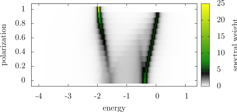
Figure 2: (Colour online) Single particle spectral function $\pi\mathcal{A}^{<}(k\approx 0,\omega)$ of the $U=4t$ Hubbard model for different polarisations as a colour-coded intensity plot, here for the metallic system with average density $n=26/32$.

Fig. 2 shows an intensity plot of $\pi\mathcal{A}(k\approx 0,\omega)$, where the $\eta$-broadened Lorentz peak was deconvoluted in a way discussed above, retaining a residual width of $0.02$ for visibility.

V Results

On the one hand, for full polarisation we recover the $\delta$-like single particle response centered at the excitation energy $\varepsilon(k\approx 0)=-2t$. Upon turning down the magnetic field, the single particle peak broadens while decreasing in height and shifting in energy. For zero polarisation, we recover the established holon peak. Thus, the trajectory for the holon-like excitation is smoothly transforming from the single electron peak into the holon peak. On the other hand, the spinon peak at $p=0$ has a more interesting behavior upon increasing the polarisation. It has a higher weight than the holon peak at $p=0$, but it shifts in energy and loses weight in accordance with the holon-like peak gaining weight. While the shoulder left of the holon-like trajectory can be attributed to the shadow band response due to $k$ not strictly zero, there is an unexpected bifurcation in the spinon-like trajectory giving rise to a second spinon-like excitation at lower energies and finite field. Its weight vanishes at some finite polarisation while the main excitation’s weight vanishes only above the critical field. Also, the spinon-holon continuum at intermediate energies develops a shoulder away from the holon-like trajectory, vanishing together with and at the spinon-like trajectory. Note that we find the same general behavior for the half-filled Hubbard model, a Mott-insulator (Fig. 3). We checked for a particular polarisation for $M=32,64,96$ sized systems that these general features are not finite size effects.

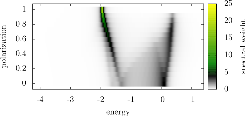
Figure 3: (Colour online) Single particle spectral function as in Fig. 2 but for the Mott-insulating state with density $n=1$.

VI Hubbard model in a trap

We add a harmonic trapping potential with $V_{\text{pot}}>0$ centered at $x_{0}=M/2$ to the Hubbard model, having then

$$H_{\text{trap}}=H+V_{\text{pot}}\sum_{i,\sigma}n_{i,\sigma}(x_{i}-x_{0})^{2}.$$

The motivation is rooted in the anticipated modelling of a Hubbard lattice model with ultra-cold fermion gases, which might involve such a trap. The single particle wave functions of the non-interacting problem ($U=0$) for the energetically lowest states are well described by Hermite functions, if the trap is not too deep ($V_{\text{pot}}(M/2)^{2}\sim t$). This leads us to use the operators

$$c_{m,\sigma}=\pi^{-\frac{1}{4}}\sqrt{\frac{g}{2^{m}m!}}\sum_{x}H_{m}(g(x-x_{0}))\text{e}^{-\frac{1}{2}g^{2}(x-x_{0})^{2}}c_{x,\sigma}$$

as single particle operators in the spectral function (1), where $g$ is a potential dependent normalisation constant and $H_{m}(x)$ is the $m$th Hermite polynomial. The level $m$ now takes the role of the momentum $k$ in $\mathcal{A}(k,\omega)$. We used a system of $M=50$ sites with $N=22$, $V_{\text{pot}}=0.01$ and tested for the removal of the lowest single particle eigenstate $m=0$ with otherwise identical parameters.

Figure 4: Single particle spectral function in the $U=4$ Hubbard model in a trap for strength $V_{\text{pot}}=0.01$ for density $n=11/50$ for different polarisations as a profile plot.

In Fig. 4 we have plotted the spectral function $\pi\mathcal{A}(0,\omega)$ for selected polarisations. Even if the terminology “spinon” and “holons” does not apply in the trapped system, we recover the same overall picture of emerging features as in the plain Hubbard model. The bifurcation exists as well, but can be seen more clearly when looking at the polarised response $\mathcal{A}^{<}_{\uparrow}$ (not shown). Finally, preliminary calculations on an extended Hubbard model with parameters as in Benthien_Jeckelmann_PRB2007 show again a similar overall picture.

VII Conclusion and Application

The main message of our result is that a magnetic field can be used to uniquely distinguish the holon and the spinon peak of the Hubbard model and thus identify the spin-charge separation. Measuring spin and charge energy scales independently is not necessary in this szenario. From zero to full spin polarisation, the spectral features of the charge sector continuously transforms into the electronic excitation spectrum, while spectral features of the spin sectors stay separate and vanish. There are, however, more facets. Firstly, our results for the trapped Hubbard model can encourage experimentalist to realise the Hubbard model on a lattice with ultra-cold gases, since even with a trap, the basic notions of spinon and holon physics remain. Secondly, in view of the results for the trapped Hubbard model and the extended Hubbard model, we conjecture that this behavior is generic for a spinful Luttinger Liquid. For integrable models this may be even analytically accessible, at least by looking at the excitation spectrum for finite magnetic field. Surprisingly, we found a bifurcation in the spinon-like response at a finite magnetic field, suggesting an underlying elementary excitation structure that is different from a simple spinon-holon picture. Further numerical results will be published elsewhere while, again, Bethe ansatz or other analytical tools may be able to reveal the nature of our finding. Finally, in view of experiments on 2D high-temperature superconductor materials Graf_Gweon_McElroy_Zhou_Jozwiak_Rotenberg_Bill_Sasagawa_Eisaki_Uchida_Takagi_Lee_Lanzara_PRL2007 trying to extract 1D interacting properties and in view of the rising interest in the FFLO state Moreo_Scalapino_PRL2007 ; Zhao_Liu_PRA2008 for attractive interaction and imbalanced systems, we find a broad range of applications and areas that may benefit from our proposal.