A spectral line survey of Orion KL in the bands 486–492 and 541–577 GHz with the Odin satellite

Abstract

Aims. Spectral line surveys are useful since they allow identification of new molecules and new lines in uniformly calibrated data sets. The subsequent multi-transition analysis will provide improved knowledge of molecular abundances, cloud temperatures and densities, and may also reveal previously unsuspected blends of molecular lines, which otherwise may lead to erroneous conclusions. Nonetheless, large portions of the sub-millimetre spectral regime remain unexplored due to severe absorptions by H₂O and O₂ in the terrestrial atmosphere. The purpose of the measurements presented here is to cover wavelength regions at and around 0.55 mm – regions largely unobservable from the ground.

Methods. Using the Odin astronomy/aeronomy satellite, we performed the first spectral survey of the Orion KL molecular cloud core in the bands 486–492 and 541–576 GHz with rather uniform sensitivity (22–25 mK baseline noise). Odin’s 1.1 m size telescope, equipped with four cryo-cooled tuneable mixers connected to broad band spectrometers, was used in a satellite position-switching mode. Two mixers simultaneously observed different 1.1 GHz bands using frequency steps of 0.5 GHz (25 hours each). An on-source integration time of 20 hours was achieved for most bands. The entire campaign consumed $\sim$1100 orbits, each containing one hour of serviceable astro-observation.

Results. We identified 280 spectral lines from 38 known interstellar molecules (including isotopologues) having intensities in the range 80 to 0.05 K. An additional 64 weak lines remain unidentified. Apart from the ground state rotational 1_1,0–1_0,1 transitions of ortho-H₂O, H${}_{2}^{18}$O and H${}_{2}^{17}$O, the high energy 6_2,4–7_1,7 line of para-H₂O ($E_{u}$=867 K) and the HDO(2_0,2–1_1,1) line have been observed, as well as the 1₀–0₁ lines from NH₃ and its rare isotopologue ¹⁵NH₃. We suggest assignments for some unidentified features, notably the new interstellar molecules ND and SH^-. Severe blends have been detected in the line wings of the H${}_{2}^{18}$O, H${}_{2}^{17}$O and ¹³CO lines changing the true linewidths of the outflow emission.

1 Introduction

Being the most popular target for spectral line surveys, in the Orion KL position OMC-1 has been the focal point of at least $\sim$20 observational efforts in the mm and submm bands over the last 20 years, starting with Johansson et al. (johansson84 (1984), johansson85 (1985)), and in the frequency range 72–91 GHz. White et al. (white03 (2003)) provide an extensive list of this earlier work in their introduction. Using the James Clerk Maxwell Telescope (JCMT), White et al. (white03 (2003)) surveyed the bands 455–469 and 492–507 GHz, surrounding the lowest frequency range of our Odin spectral scan (486–492 GHz). The frequency range 607–725 GHz, just above the Odin spectral scan band 542–576 GHz, has been surveyed by Schilke et al. (schilke01 (2001)) using the Caltech Submillimeter Observatory (CSO).

More recent additions include 159.7–164.7 GHz (Lee & Cho lee02 (2002)), 795–903 GHz (Comito et al. comito05 (2005)), 260–328 GHz (Yoshida & Phillips IAU 231), and an IRAM 30 m survey (168 GHz in three windows between 80 and 281 GHz) by Tercero et al. (IAU 231¹).

The first imaging line survey of Orion KL in the submm range (337.2–339.2 and 347.2–349.2 GHz) was recently reported by Beuther et al. (beuther05 (2005)), who used the Submillimeter Array interferometer. They later employed the same instrument to make measurements around 680 and 690 GHz with similar bandwidths (Beuther at al. beuther06 (2006)).

The luminous Orion Kleinmann-Low infrared nebula (Orion KL; $L\approx$10${}^{5}\,L_{\sun}$), and its surrounding molecular cloud, is the nearest (distance of 450 pc) and probably most studied massive star formation region in the sky. A very useful review has been written by Genzel and Stutzki genzel89 (1989); for reference updates see e.g., Olofsson et al. olofsson03 (2003), and Wirström et al. wirstroem06 (2006). Here we summarise some source component designations and dynamical properties particularly relevant to the molecular line identification work in the current presentation of our Odin spectral scan data, which includes our molecular line assignments (in the Online Table 4).

Odin’s circa 126″ antenna beam is centred on the most prominent infrared ‘point’ source in the KL nebula, IRc 2 (R.A. 05^h35^m14$\aas@@fstack{s}$36, Dec. -05°22′29$\aas@@fstack{\prime\prime}$6 (J2000)). The Orion hot core source, with a size of only $\approx$10″ and centred only 2″ S of IRc 2, is a warm ($\approx$200 K, or even higher; cf. Sempere et al. sempere00 (2000)), dense ($\approx$10⁷ cm^-3) clump or rather collection of clumps, characterised by a spectral line width of 5–15 $\rm km\,s^{-1}$ centred on $v_{\rm LSR}$=3–6 $\rm km\,s^{-1}$ and exhibiting emission from nitrogen-containing species at markedly enhanced abundances. The outflowing gas, or the plateau source, with a size of 40-60″, may be characterised in terms of a bipolar high-velocity flow elongated in the SE-NW direction (reaching velocities of $\pm$100 $\rm km\,s^{-1}$), and a SW-NE extended low-velocity flow (the ‘18 $\rm km\,s^{-1}$ flow’) of size 15–30″, centred on 10 and 5 $\rm km\,s^{-1}$, respectively. Further details on the complex structure of the outflow – such as a central jet and localised ‘bullet’ type emission within the high velocity flow – are nicely revealed by the IRAM 30-m CO J=2-1 maps by Rodríguez-Franco et al. (rodriguez99 (1999)). Within the Odin 126″ antenna beam there is also an N-S extended quiescent molecular cloud structure (the ridge), with densities of 10⁴–10⁶ cm^-3 and temperatures in the range 20–60 K, and characterised by line widths of 3–5 $\rm km\,s^{-1}$ and an abrupt velocity shift across the KL nebula from $v_{\rm LSR}$=8 $\rm km\,s^{-1}$ (in the south) to 10 $\rm km\,s^{-1}$ (in the north). The large-scale chemical structure of many important ridge molecules is outlined in Ungerechts et al. (ungerechts97 (1997)).

The interaction between the bipolar high-velocity outflow and the surrounding ridge gas produces shock heating and shock enhanced chemistry, markedly visible in terms of bright H₂ emission, strong high-$J$ CO lines and uniquely strong emission from abundant H₂O (Melnick et al. melnick00 (2000); Olofsson et al. olofsson03 (2003)). Also the roughly orthogonal low-velocity outflow component appears to interact with the ambient gas, creating density, temperature and column density enhancements in the ridge gas. One such feature is the compact ridge cloud ($\Delta{}v$=3 $\rm km\,s^{-1}$; $v_{\rm LSR}\approx$8 $\rm km\,s^{-1}$) situated only 10–15″ S of IRc 2, on the northern tip of the 8 $\rm km\,s^{-1}$ ridge cloud, where complex oxygen-containing molecules have been observed to be abundant. The hot core itself might also be a result of shock-induced compression. A recent finding along these lines is enhanced [CI] forbidden line (³P₂–³P₁) emission north and south of IRc 2 (in a shell of radius $\approx$20″, where the outflow encounters ambient gas), and proposed to result from CO dissociation in shocks (Pardo et al. pardo05 (2005)).

Although the major source constituents are commonly discussed in the literature as outlined above, we caution readers that observations yielding higher spatial resolutions (e.g. Blake et al. blake96 (1996); Wright et al. wright96 (1996); Beuther et al. beuther05 (2005), all employing aperture synthesis) reveal that the KL core composition is in fact more complex and breaks down into further sub-structures of sizes $\lesssim 10^{3}$ AU.

We present here the observational results and line identifications. Numerical analyses such as column density and rotation temperature estimates are included in an accompanying paper in this A&A issue (Persson et al. persson06 (2006), Paper II hereafter).

2 Observations

The present data-set was obtained in a four-part campaign running over 1.5 years, starting in spring 2004 (Feb.–Apr.), followed by fall 2004 (Aug.–Oct.) and continuing in the same manner in 2005. This division naturally arises from the combination of source coordinates and Odin’s orbital plane (Sun-synchronous low Earth orbit) leading to seasonal visiblilty constraints for low-declination sources such as the Orion nebula.

The dedicated observing period spanned over $\sim$1100 revolutions with a very high success rate due to consistently stable spacecraft performance. Each orbit allows 61 minutes of astronomical observations, whereas the source line-of-sight is occulted by the Earth and its atmosphere for the remaining 35 minutes of the orbital period. We employed position switching (PSW) in order to acquire cold sky reference spectra. This was implemented by regularly reorienting the entire spacecraft by $-$15′ in RA with a cycle time of 1 minute, carried out by the onboard momentum wheels. The resulting efficiency penalty for slew time was low ($<$20%).

The beam size and main beam efficiency of Odin’s 1.1 m offset Gregorian telescope at 557 GHz are 2′1 and 0.9, respectively, as measured in continuum observations of Jupiter assuming a Jovian brightness temperature of 145 K and a disc-like source geometry (Frisk et al. frisk03 (2003)).

The pointing is maintained in real time by the attitude control system, assisted by two star trackers with an angular separation of 40°. It has been empirically established that the reconstructed attitude uncertainty is $\leq$15″most of the time.

There are four tunable submm receivers of single-sideband (SSB) type in the radiometer, all of which were employed for these measurements. Image band rejection is achieved using Martin-Puplett filters with cooled termination absorbers and Schottky mixers are used for frequency down-conversion. The channels have centre frequencies of 495, 549, 555, and 572 GHz and the design of the receiver system allows simultaneous use of RX555 and RX572, or RX549 and RX495 (Frisk et al. frisk03 (2003)).

The tuning range of 14 GHz was not fully exploited in all channels although the combined results from the complementary pair RX549 and RX555 cover all their accessible frequency range. System temperatures in the passband centres were around 3000–3500 K with few exceptions as measured by switching between the main beam and a hot load at room temperature. For a given tuning, $T\!\!_{\mathrm{sys}}$ does not change in time by more than a few percent due to the stable conditions and no interfering atmosphere.

The observing strategy was to tune the receivers in 0.5 GHz steps and observe for 25 orbits. The resulting overlap in between adjacent tunings gives a net on-source integration time of 50$\times$61$\times$0.8/2$\approx$20h per channel. This commonly used approach was adopted to reduce potential impacts of artificial spectral patterns/transients or baseline effects which could arise in one tuning but conceivably not in both.

Three spectrometers were used: one acousto-optical spectrometer (AOS) and two hybrid autocorrelators (AC1/2). The former has a bandwidth of 1.1 GHz and a channel spacing of 620 kHz, while the latter two can be used in several modes. In the low resolution mode used here, the bandwidth is 700 MHz with 1 MHz channel spacing. The AOS and the ACs have rather different characteristics and therefore we have used slightly different approaches in building the final spectra, hence the division into two parts of the next section.

3 Data reduction

The data reduction has been performed in two parallell, independent efforts by members of the Odin Team situated at the Onsala Space Observatory and in the University of Calgary. The spectra presented in this paper are the products of the data reduction at Onsala. The very similar Calgary results have been used to verify the quality of the spectra shown here. Although a few differences were found for lines at a level below 0.1 K (or below 4$\sigma$ in terms of the baseline noise), we are encouraged to believe that the majority of such weak lines are real.

3.1 AOS and data from RX549/RX555

3.1.1 Calibration and averaging

There were essentially three complicating factors that needed special consideration in these data sets.

Frequency correction:

By using telluric ozone and water (and occasionally rarer lines during the occultation phase, the capability exists to check the frequency setting to a very high accuracy, as is illustrated in Fig. 1.

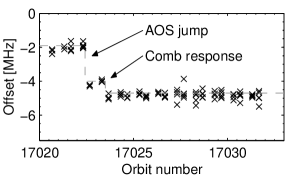
Figure 1: Tracing the frequency deviation using the telluric H${}_{2}^{17}$O line. As is evident, there was an early sudden shift of the line position, corresponding to an AOS laser mode jump during warming up – a small penalty because of our shared astronomy/aeronomy mission. The times of such shifts can be determined accurately since they affect the total power levels of the spectrometer. The gray dashed line shows the correction applied to the data from this sample observation.

It was found that there was an offset of 0–5 MHz from the commanded value leaning towards the upper value most of the time. Furthermore, on a few occasions the offset was seen to change instantaneously by 2–3 MHz in mid-observation between two apparently stable offset levels. Thus it was deemed necessary to register telluric frequency references at all times and correct the astronomical spectra accordingly. If no atmospheric lines were present in a particular tuning, overlapping astronomical lines inherent to a different but adjacent tuning with a known frequency correction, were cross-correlated to find the proper correction. This method gave consistently positive results and we now believe that the absolute frequency uncertainty is 1 MHz ($\approx$0.5 $\rm km\,s^{-1}$) at worst.

Channel dependent RMS:

Probably owing to the large bandwidth of the AOS, the system temperature profiles had rather steep gradients towards the upper and lower edges, often leading to noise temperatures in these portions twice the mid-spectrum values. When averaging together two adjacent tunings, the low-noise central channels from one tuning will be combined with the high-noise edge channels of the other. This has been taken into account in the weighting procedure by letting the most recently measured $T\!\!_{\mathrm{sys}}$ profile represent the formal noise in each channel of the the next spectrum to be included in the average. Provided that the integration times and resolutions are all the same, and that we have a good linear correlation between $T\!\!_{\mathrm{sys}}$ and the channel RMS, this approach is easily justified.

Side-band suppression:

In general, we have very good suppression of the undesired image band ($\gtrsim$20 dB in at least one tuning). In the RX555 tunings, there is one exception where the appearance of an image SO line indicates a suppression of only 10 dB. Similarly poor SSB suppression was seen more frequently in the RX549 data through the emergence of telluric image ozone lines in occultation phase data. As is evident in the final result, we had in general more problems with high $T\!\!_{\mathrm{sys}}$ and unexplained baseline ripples in this frontend/backend configuration, probably related to the poorer SSB performance. In those cases where image lines were seen in the final average (almost exclusively due to the strong H₂O and ¹³CO lines at 557 and 551 GHz, respectively), the appropriate channels were excluded to remove the interference. The complementary tunings certified that no gaps were created in the total average, although the noise is visibly higher in these portions due to less net observing time. Potential low-level image line intrusions are in general sufficiently weakened not to be seen in our baseline noise, owing to the satellite motion Doppler correction which serves to disperse image band signals.

Other pre-averaging measures consisted of first linearising the readouts of the AOS aided by internal frequency comb measurements, then resampling the AOS spectra to whole MHz to match the AC resolution.

The individual spectra each represent one on-source observation in the PSW cycle which is equivalent to 24 s integration time. During one such observation, the variation of the projected satellite orbital velocity in the direction of the source is not taken into account which introduces a slight spectral smearing of astronomical lines. However, the magnitude of the Doppler shift change at most amounts to $\sim$200 $\rm m\,s^{-1}$ and is considerbly less for the major part of the orbit.

The baseline stability was very good (Sect. 3.1.2) and no fits were subtracted from the spectra in the averaging procedure. However, to obtain accurate line property estimates for the very weak features, we opted to subtract a piecewise linear fit from the broadband end products, putting the baseline level at zero around clearly detected emission lines.

3.1.2 Baseline stability/continuum level

We have estimated the dust continuum beam averaged antenna temperature around 550 GHz using the spectra from the RX549 and RX555 receivers. One value was extracted for each tuning as shown in Fig. 2 and the average amounted to $T_{\rm A}$=0.45 K (1800 Jy beam^-1).

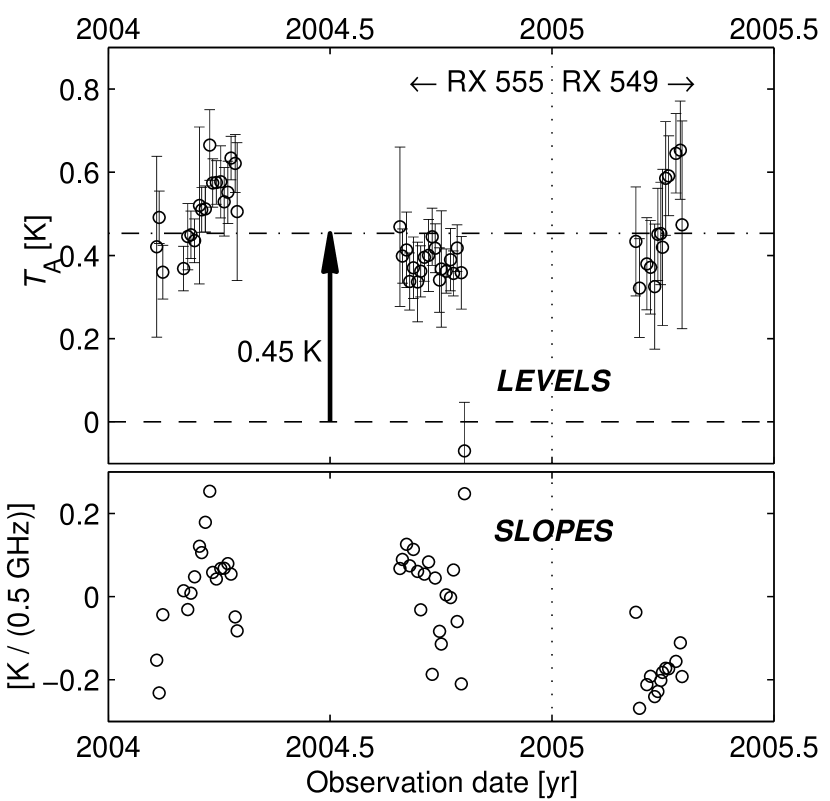
Figure 2: Baseline levels and slopes in 52 RX555 and RX549 observations before any baseline subtractions. The error bars in the upper panel correspond to 3$\sigma$. The slopes are measured as the level difference of two halves of the spectra whose centres are separated by 496 MHz. This figure indeed highlights the stability of the receiver/AOS/calibration chain, but the upwards trends of the levels towards the ends of both spring observing runs remain unexplained. There is also an observation that inexplicably appears to lack continuum signal (while telluric spectral lines could still be detected).

Due to the crowding of strong lines in some tunings, this calculation relied on noise statistics and did not require that the positions of lines were known beforehand. The assumptions made were instead i) at least half the channels in a spectrum were largely unaffected by emission lines, ii) the baselines are largely flat compared to the noise scatter of the intensity in individual spectra, and iii) the noise is Gaussian and the RMS is well described by its formal value derived from the radiometer formula.

The simple procedure was then to sort all channels according to increasing intensity and select the bottom half of the distribution (the top half is ‘contaminated’ by emission lines). Statistically, the expectation value of the distribution is then found by adding 0.8$\times$RMS_formal to the mean value of the selected low-intensity channels.

To further remove effects of baseline variations, and to get a handle on the baseline stability, each spectrum was divided into two 500 MHz subspectra on which the calculation described above were performed. The average difference between the two halves in each tuning then additionally supplied an indication of the first order trend (or slope) of the baselines. Figure 2 also illustrates the results found here. Although it is obvious that a systematic baseline pattern was present throughout the RX549 observations, the RX555 baseline performance is quite satisfactory.

3.2 ACs and data from RX495/RX572

The 700 MHz AC spectra are created by stitching together seven 112 MHz portions. To achieve the double coverage of each frequency interval as we do with the AOS, one AC was split into two portions, 3+4 subbands, and placed on each side of the other AC that covered the central 700 MHz in the passband.

Each such sub-band is typically “well behaved” in terms of having Gaussian noise and a uniform gain curve. However, in the PSW observing mode there is for unknown reasons a linear falloff in channel intensity from the start of each on and off sequence. Due to the inescapable slight asymmetry between on and off measurements, and to the fact that the drift rate changes gradually over the channels in one sub-band, the calibrated spectra end up with a low-level curved saw tooth-like appearance with two sub-bands forming each tooth. This pattern has been removed by using high-order polynomials after careful comparisons with the results obtained by calibrating each sub-band separately. Around the extremely broad CO line at 576.3 GHz, this method failed and the corresponding two tunings were instead cured by employing a corrective procedure that nullifies the effects of the intensity drift mentioned above but is very time-consuming.

The uppermost 200 MHz of the RX495 spectrum were acquired from a tuning that suffered instability; the LO alternated between being properly locked and oscillating between frequency offsets of $\pm$33 MHz. Using the recorded IF current and the amplitudes of the [CI] forbidden line line at 491.7 GHz (visible in individual spectra, $T_{\rm A}$$\approx$6 K) as guides, about ten minutes of integration was recovered. In spite of the higher noise level thus obtained, we chose to include this spectral section since it contains two strong lines, the [CI] and a low-energy methanol transition ($T_{\rm A}$$\approx$1.2 K).

We did not find any evidence of image band lines interfering in the signal side band for these two receivers, nor did we find any significant frequency offsets (at most $\approx{}1\,$MHz) from nominal values in telluric line position controls in sample tunings.

4 Results

4.1 Summary

Table 1 lists some general figures and characteristics for the survey as a whole.

Table 1: Survey overview

Property	Value
Bandwidth covered	42 GHz
Number of lines detected	344
Line density	8 GHz-1 (range: 4–20)
Line intensity range	0.05–80 K
Number of species detected	38
Typical RMS reached	$\sim$25 mK/1 MHz channel
Total $\int\!{}T_{\mathrm{A}}\,{}dv$	2 455/2 525 K $\rm km\,s^{-1}$
Total line luminosity	5$\times$1026 W
Mean line-to-continuum ratio	0.2

As is evident from this Table, our integrated intensity is dominated by the continuum emission by a ratio of 5:1 (see Sect. 3.1.2 for details). The line-to-continuum ratio found here, 20%, is much lower than that at 350 GHz, 50%, but rather close to the 15% found at 650 GHz (Schilke et al. schilke01 (2001)). For a larger telescope (such as the Herschel Space Observatory) one can expect this value to increase somewhat due to increased intensity from the abundant lines from the compact line sources ($<$10″) compared to the dust continuum source whose KL component is about 30″ as seen in for example the 345 GHz bolometer map of Siringo et al. (siringo04 (2004)).

4.2 Spectra and identifications

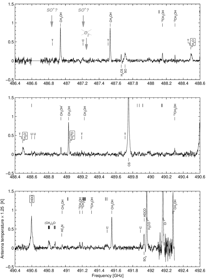
Figure 3: The Odin spectral survey between 486.4 and 492.1 GHz (RX495). Note the intensity scaling factor of 1.25 to approximately deconvolve the spectrum to the beam size near 557 GHz (assuming a point source). Empty markers at the intensity level of 1.25 K denote CH₃OCHO lines.

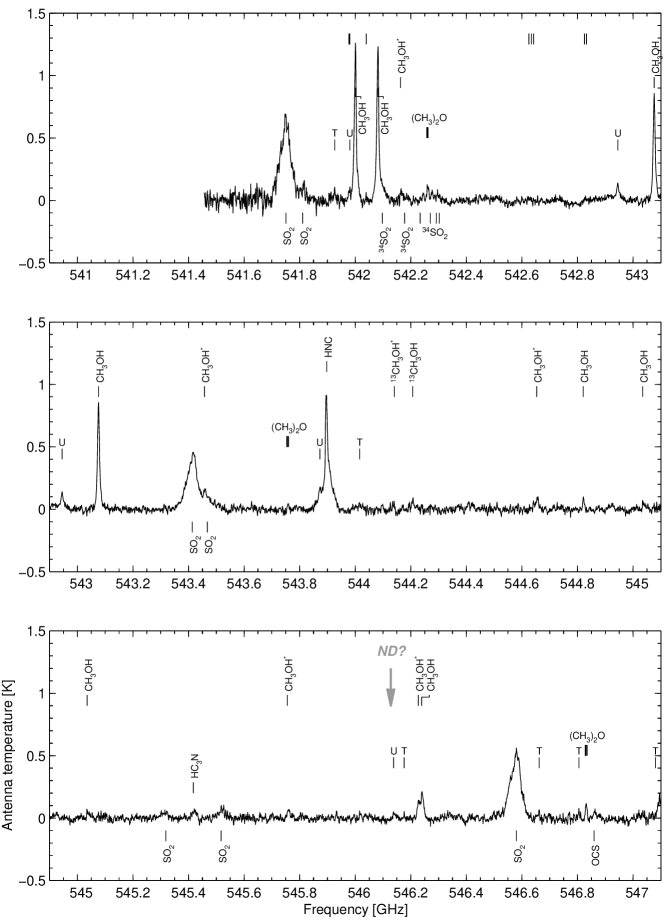
Figure 4: The Odin spectral survey between 541.4 and 547.1 GHz (RX549). Empty markers at the intensity level of 1.25 K denote CH₃OCHO lines. A star denotes a transition within a vibrationally excited state: $v_{\rm t}$=1 for methanol, and $\nu_{\rm 2}$=1 for SO₂.

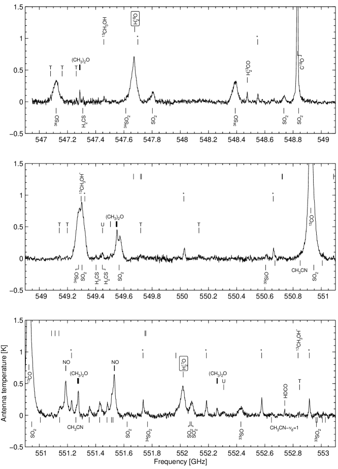
Figure 5: The Odin spectral survey between 546.9 and 563.1 GHz (RX555). Unlabelled markers at intensity levels -0.1, 0.5, 0.9, and 1.25 K, belong to SO₂, (CH₃)₂OH, CH₃OH, and CH₃OCHO, respectively. A star denotes a transition within a vibrationally excited state: $v_{\rm t}$=1 for methanol, and $\nu_{\rm 2}$=1 for SO₂. Two sets of markers immediately below the spectrum baseline belong to ground state and vibrationally excited CH₃CN.

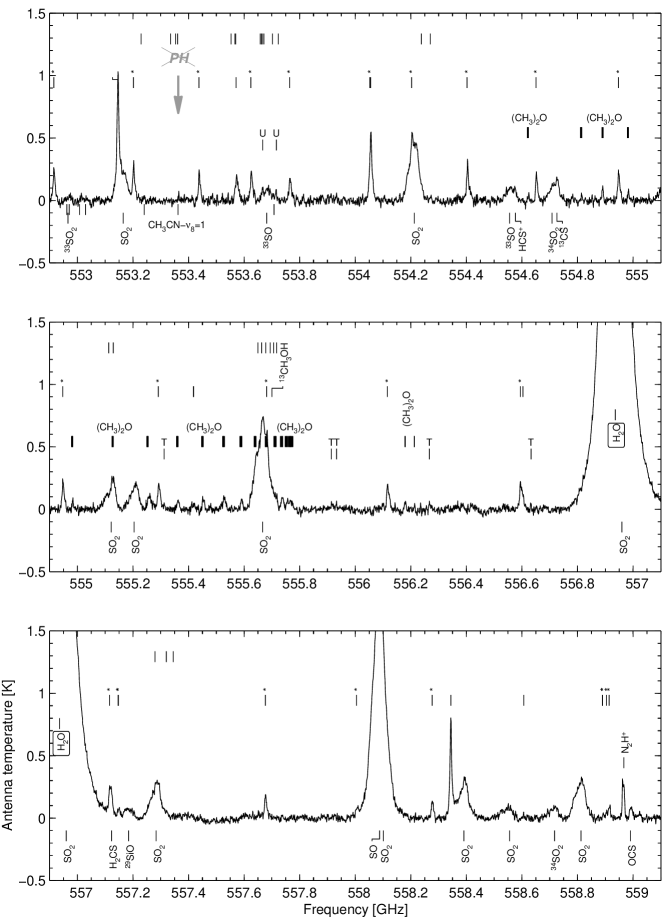
Figure 5: continued.

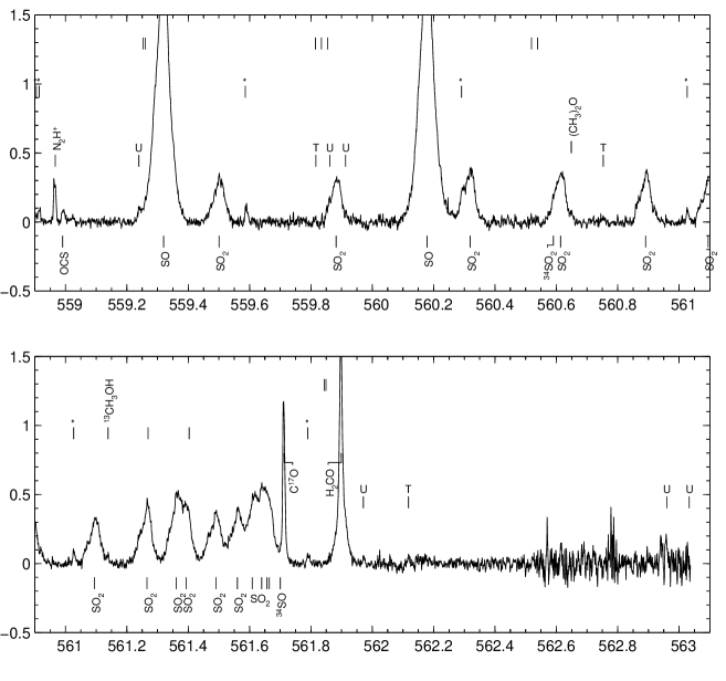
Figure 5: continued.

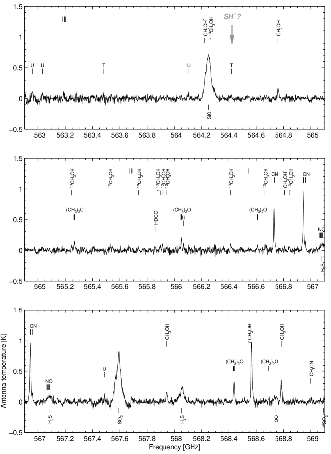
Figure 6: The Odin spectral survey between 562.9 and 577.6 GHz (RX572). Empty markers at the intensity level of 1.25 K denote CH₃OCHO lines.

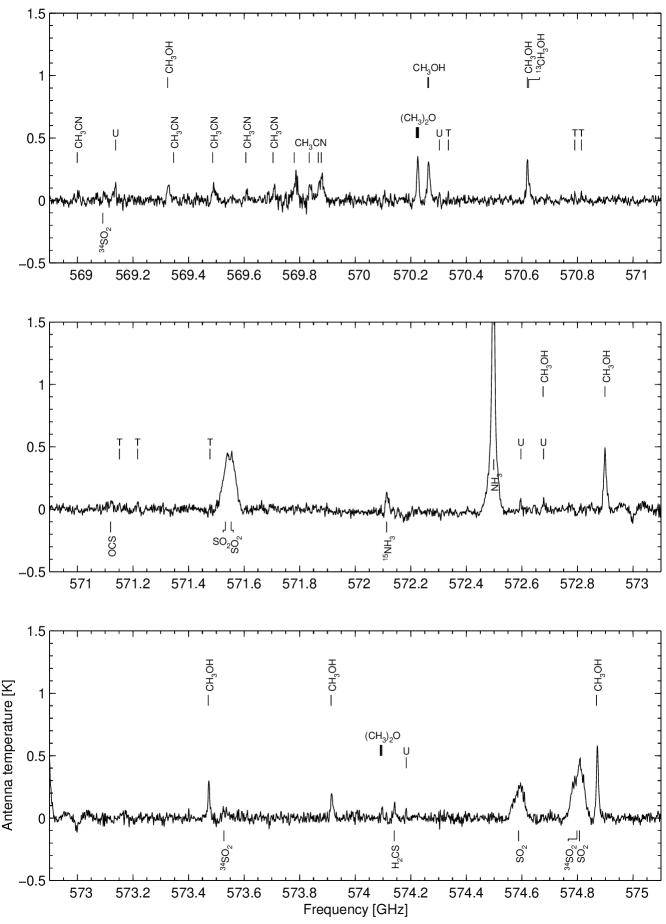
Figure 6: continued.

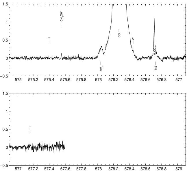
Figure 6: continued.

The final spectral scan results from the four receivers can be seen in Figs. 3, 4, 5, and 6. The frequency scale is counted w.r.t. a source velocity of $v_{\rm LSR}$=$+$8 $\rm km\,s^{-1}$, and markers are placed at the laboratory rest frequencies of the transitions attributed to the line features.

The general method for identification was to select the most plausible species after comparisons with available molecular databases (SLAIM03: Lovas lovas03 (2003); CDMS: Müller et al. mueller01 (2001); JPL: Pickett et al. pickett98 (1998)) of predicted/calculated or directly measured transition frequencies (SLAIM03 contains both kinds wherever available). The selection criteria included: frequency coincidence, expected abundance, line strength, line width, line velocity, and upper state energy. Where possible we have also used rotation diagram analysis (cf. Goldsmith & Langer goldsmith99 (1999)) to guide our identification, as discussed in Paper II.

In the case of marginally detected line features suspected to arise from more complex molecules such as dimethyl ether and methyl formate, we also required that other lines of similar expected emission characteristics be visible at other frequencies within the observed bands.

It is important to note that any conceivable artificial sharp features produced in the radiometer would likely be stable in the sky frequency rest frame and thus would be significantly smeared here since the satellite motion Doppler correction of each spectrum varies between -7 and +7 $\rm km\,s^{-1}$ over one orbit.

The line counts, upper state energy ranges and total integrated intensities for each detected molecule are listed in Table 2. All identifications (molecule and laboratory rest frequency) can be found in Table 4 (available on-line).

Table 2: Summary of all detected species.

Species	Number	Energy range	$\int\!{}T_{\mathrm{A}}\,{}dv$
		[K]	[K $\rm km\,s^{-1}$]
CH3OCH3	47	106-448	18.3
SO2	42	75-737	239.9
34SO2	5	79-457	2.6
SO	5	71-201	181.5
33SO	3	191-199	6.5
34SO	2	191-197	15.6
CH3OH $v_{\rm t}$=1	42	332-836
CH3OH	34	38-863	108.6
13CH3OH	21	37-499	6.8
13CH3OH $v_{\rm t}$=1	2	373-670
CH3CN	17	410-1012	9.3
NO	12	84-232	11.1
CN	8	54	8.5
H2CS	5	138-343	1.7
H2CO	3	106-133	38.5
H${}_{2}^{13}$CO	1	130	0.6
HDCO	3	114-141	2.8
OCS	3	604-658	1.3
$o$-H2O	1	61	320.3
$p$-H2O	1	867	2.2
$o$-H${}_{2}^{17}$O	1	61	9.4
$o$-H${}_{2}^{18}$O	2	60-430	16.2
HDO	1	66	10.7
HC3N	2	648-799	0.6
CO	1	83	1100
13CO	1	79	174.3
C17O	1	81	6.0
C18O	1	79	24.3
C	1	24	38.7
NH3	1	27	20.6
15NH3	1	27	0.7
HNC	1	91	10.7
N2H+	1	94	1.5
H2S	1	166	4.4
CS	1	129	24
13CS	1	173	v blend
SiO	1	190	17.6
29SiO	1	187	1.4
30SiO	1	185	0.5
HCS+	1	186	v blend
NS	1	442	v blend
U-line	28	-	9.1
T-line	36	-	7.2

Also of interest here are the spectral offsets of the measured lines relative to the laboratory frequencies. We have estimated these from the value found at the peak intensity channel of the lines (assuming a systemic emission velocity of +8 $\rm km\,s^{-1}$) and they are listed in full in Paper II. The average offset per molecule is $-$0.6 MHz but this cannot be used as a quality measure of the data fidelity nor the accuracy of tabulated rest frequencies since different molecules emit at different velocities (as is likely reflected by the high dispersion, 3.2 MHz). In addition, these emission velocities are often instrument-dependent due to varying beam fillings of the different source components. Nonetheless, by choosing the 35 strongest lines of methanol (which conveniently has narrow emission lines), we minimise this effect and get a dispersion of only 1.1 MHz. While this is slightly higher than the stated estimated frequency uncertainty of our spectra, there are a number of possible remaining explanations aside from data error such as lab measurement/calculation error and line blending.

4.3 Important line blends

A means to identify and subsequently remove ‘interfering’ lines is helpful, particularly in the detailed study of line shapes (where the signal-to-noise ratios of the lines are such that this is feasible).

It now seems convincingly clear that the line wings of the rarer isotopologues of water and carbon monoxide are affected by emission from SO₂, ³⁴SO₂, CH₃OH and CH₃CN. Fortunately, the emission from these species can be accurately modelled due to the wealth of other lines from these species present in our band, allowing determinations of column densities and excitation temperatures. We have in the course of our analysis tried to reconstruct the true shapes of some lines by subtracting polluting emissions from our spectra, and in Paper II one successful example is demonstrated (H${}_{2}^{17}$O).

We caution that this approach is only useful in contexts where the interfering lines emit in an optically thin portion of the main line (or if the gas is stratified so that the optically thin line arises in the near side of the gas column). For instance, we do not find it likely that the SO₂ line at 556.960 GHz significantly alters the profile of the main water line (at 556.936 GHz) since i) the optical depth towards the centre of the water line is very large, and ii) according to the interpretation in Olofsson et al. (olofsson03 (2003)) the High Velocity Flow as seen in water is located in front of (or around) the Low Velocity Flow from which the sulphur oxide lines mainly originate, as evidenced by their line widths and source size.

4.4 Unidentified line features

We have defined U-lines – clearly detected lines well distinguished from the baseline noise – and T-lines, which are only marginally visible (T for ‘Tentative’) against the noise, or in an apparent line blend. The lines of both types are marked in the spectra and listed in Table 3.

Table 3: Unidentified (U) and/or marginally detected (T) lines

Frequency	Type	Sugg.	Table
[MHz]	[U/T]	ident.	continued
486845	T	SO+	555914	T	—
487209	U	SO+	555933	T	—
487507	T	CH3CHO	556267	T	—
488477	T	—	556633	T	—
488598	U	CH3OCHO	559239	U	CH3OCHO
488633	U	CH3CHO	559816	T	HDO
489193	T	—	559861	U	CH3OCHO
489709	T	SiS	559913	U	—
491496	U	CH3OCHO	560753	T	—
491892	U	—	561971	U	—
541926	T	—	562118	T	—
541981	U	CH3OCHO	562960	U	—
542945	U	—	563033	U	—
543873	U	—	563481	T	HNCO
544016	T	SiS	564105	U	—
546138	U	ND	564418	T	SH-
546176	T	ND	566066	U	—
546662	T	—	567485	U	—
546805	T	—	569138	U	HNCO
547080	T	—	570303	U	—
547162	T	—	570335	T	—
547262	T	HNCO	570790	T	—
549142	T	HNCO	570814	T	—
549199	T	HNCO,H2CS	571151	T	HNCO
549449	U	—	571217	T	HNCO
549719	T	SO2,(CH3)2O	571477	T	H2C18O
550132	T	SO2	572596	U	—
552308	U	—	572678	U	—
552846	T	—	574184	U	—
553667	U	CH3OCHO	575397	T	—
553716	U	—	576446	U	—
555312	T	—	577160	T	—

We have in some cases found candidate species (Table 3) which have not fulfilled all our criteria for an unequivocal designation and they are kept as U- or T-lines. Some of the more interesting scenarios are discussed below.

4.4.1 New SO⁺ lines?

Interstellar SO⁺ was first detected in the shocked clump IC443G, presumably being formed in the dissociative shock caused by the supernova remnant (Turner turner92 (1992)). Our weak unidentified lines at 486.845 and 487.209 GHz tentatively can be identified as the $J$=21/2–19/2 $e$ and $f$ doublet of the reactive radical SO⁺ in its ${}^{2}\Pi_{1/2}$ ground state (JPL; Amano et al. amano91 (1991)). The suggested assignment is consistent with the detection in Orion KL of lower energy SO⁺ lines at 115.804, 116.180, 208.590, and 255.353 GHz (Turner turner94 (1994)). Our assignment is further strengthened by the U-line at 347.743 GHz observed by Schilke et al. (schilke97 (1997)) which we identify here with the $J$=15/2–13/2 $e$ transition of SO⁺ at 347.740 GHz. However, the corresponding $f$ transition at 348.115 GHz is hidden in a blend with ¹³CH₃OH and ³⁴SO₂.

4.4.2 Other notable frequency coincidences:
SH^- and ND

Our weak, slightly broad lines near 546.138 and 546.176 GHz could be associated with the $N_{J}$=1₁–0₁ hyperfine transition cluster of the ND radical in its $X^{3}\Sigma^{-}$ ground vibronic state (CDMS; Saito & Goto saito93 (1993); Takano et al. takano98 (1998)). If so, the strongest component is at a blue-shifted position closer to the Hot Core velocity, in agreement to what is seen in other nitrogen hydrides such as NH₂ (which we tentatively conclude to be blue-shifted after studying the 900 GHz spectral survey of Comito et al. comito05 (2005) in detail). NH₃ on the other hand – discussed further in Paper II – has a $\sim$60% Hot Core contribution but this is heavily masked by its optical depth in both the Hot Core and in the Compact Ridge. Unfortunately, the predicted shape of the line bundle as a whole does not match the observation and one would need to invoke non-LTE excitation to explain this difference.

A weak unidentified line at 564.418 GHz may originate in the $J\!=\!1\!-\!0$ rotational transition of SH^- in its $X^{1}\Sigma^{+}$ ground state, measured to fall at the frequency 564.422 GHz (Civiš et al. civis98 (1998)). A new interstellar anion would be of utmost interest since only one has been found previously, namely the discovery of C₆H^- which was recently reported by McCarthy et al. (mccarthy06 (2006)). Thus – although our line is not strong enough to claim a detection ($\sim$3.5$\sigma$ relative to the local noise) – we chose to perform a very simple column density calculation (or an upper limit thereof if the line turned out false). By employing the LTE assumption with full beamfilling, an excitation temperature of 100 K, and a dipole moment of 0.273 D (adopted from the ab initio calculations of Senekowitsch et al. senekowitsch85 (1985)), we arrive at a figure of $N_{\rm SH^{-}}$=2$\!\times\!$10¹³ cm^-2. The scenario used would be consistent with SH^- residing in the extended OMC-1/M42 face-on PDR (discussed in Wirström et al. wirstroem06 (2006)). Should the origin of the line (if real) be any of the smaller Orion KL components – as indeed the observed line width ($\Delta{}v_{\rm FWHM}$=11 $\rm km\,s^{-1}$) seems to indicate – the column density rises by a factor of $\sim$200. We deem at least the PDR column density to be a reasonably low value in light of the rather unknown chemistry of similar hydrides in the interstellar medium. The SH radical, for instance, has only been found in the atmosphere of a Mira variable through mid-IR transitions (Yamamura et al. yamamura00 (2000)). Nevertheless, a possible contribution from SH in a C₃ spectrum towards Sgr B2 has been reported by Cernicharo et al. (cernicharo00 (2000)). We also note that a formation pathway exists involving H₂S (via dissociative electron attachment), a molecule observed by Odin in the present survey and treated in Paper II.

Both these candidates (marked by gray arrows in the spectra figures) can be confirmed or ruled out by the forthcoming Herschel mission (discussed further in Sect. 5). For the case of ND, the triplets of NH at 947 and 1000 GHz are also relevant.

4.5 Non-detections

Two notable non-detections have been indicated by gray arrows in our spectra: the PH and O₂ molecules. The PH line (a hyperfine transition within the $N_{J}$=1₁-0₁ group at 553.363 GHz) has also been searched for in IRC$+$10216 by Odin to a much higher sensitivity by Bernath et al. (bernath07 (2007)), and we refer to them for details on the PH physical and chemical properties and its role in the circum- and interstellar medium. The O₂ line at 487.249 GHz has previously been searched for by the SWAS satellite (having a larger beam size) down to a sensitivity of 6.4 mK (Goldsmith et al., goldsmith00 (2000)) without success. Both O₂ non-detections are consistent with the Odin upper limit from the ground state transition at 118.750 GHz by Pagani et al. (pagani03 (2003)).

4.6 Improvements of existing spectroscopic data

In the case of our rather weak H₂CS lines, we did at first find frequency offsets between 6 and 14 MHz systematically red-wards of the expected values (as given in the JPL database which indeed stated high uncertainties for these calculated H₂CS frequencies). Prompted by private communication, an entry for this molecule was subsequently inserted into CDMS and the new calculated rest frequencies found there gave very good agreements with our measured positions in all but one line. This is an encouraging result proving that large measured frequency offsets are likely not to be spurious and may in some cases indicate that the existing tabulated spectroscopy data are off the mark.

In the case of H₂CS, new extensive laboratory spectroscopy work has kindly been performed by Eric Herbst and his collaborators. The resulting H₂CS database will be crucial for Herschel Space Observatory.

In general, we hope that our measured line parameters (listed in bulk in Paper II) may be useful for accurate determination of molecular data such as rotational constants.

5 Discussion of future observations

No further Odin observations of this kind are currently planned and the observation time cost for significant noise reduction would in any case be prohibitive. However, the spectral portions presented here will be reobserved by the Herschel space observatory and is of interest to briefly discuss what they could obtain. Herschel is a European Space Agency (ESA) satellite mission aimed at launching a 3.5 m telescope equipped with very low noise submm/far-IR heterodyne receivers in 2008.

Most of the identified lines in this survey belong to species already observed at other transitions (at both lower and higher frequencies) and source size estimates for the corresponding emission components are available in the literature (e.g. references in Sect. 1 and Paper II). A rough Herschel beam-filling estimate based on these source sizes reveals that those lines will be 1–10 times stronger in the Herschel spectrum, with the majority leaning towards the higher end. Assuming further an observation time of only one hour in combination with recent figures for the Herschel receiver system sensitivity, one finds that the signal-to-noise ratio will be increased by up to a factor of 20 in such a case. This will be particularly useful for the weakest lines (5–10$\sigma$) seen in the Odin survey which will be possible to study in some detail in the Herschel spectrum. It is in this group we find nearly all the unidentified lines and the potential for new discoveries among them is obvious. The interesting frequency coincidences of SH^- and ND described earlier are good examples. The interpretation of these and even weaker lines runs, however, the risk of being hampered by line crowding and blending (already up to 20 lines/GHz in our spectrum) due to the plethora of lines that will emerge from the noise compared to the Odin spectrum. This in turn will put high demands on the system baseline stability in order to correctly disentangle the emissions. The pollutive contributions in the key water isotopologue lines discussed above will also be worsened (due to differential beam-fillings) and on a side note one can predict that this problem will arise in most sources where Herschel observes these species.

6 Conclusions

We have conducted a spectral survey in two submillimetre windows largely inaccessible from the ground due to atmospheric opacity. The frequency ranges covered are: 486.4–492.3 and 541.5–577.6 GHz. This was achieved using the Odin submm satellite.

The spacecraft performance was generally excellent in terms of high observing efficiency and good sideband suppression most of the time (within the SSB receivers).

The baseline stability has been shown to be satisfactory, albeit high-order polynomials being required in about 50% of the data to remove a fixed pattern arising in the autocorrelators in this particular observation setup.

Careful attention has been paid to the frequency alignment of our data resulting in an estimated frequency error of $\lesssim$1 MHz.

Thus, high confidence is warranted in the fidelity of the reduced spectra. To ascertain the calibration accuracy, some lines have also been compared to previous or later targeted Odin observations using markedly different instrumental setups.

We found a total of 280 identified emission lines (some of which include multiple transitions), and 28 unidentified lines. We have also pointed out a further 36 borderline detected features which in some cases have interesting candidate assignments such as SH^- and SO⁺.

Among the 38 detected molecules, we have four water isotopologues seen in at least five emssion lines. These data are used in Paper II to make a water abundance analysis.

Column density estimates for all species are presented in Paper II, as well as abundance, source size, and rotation temperature estimates for a selection of molecules.

Appendix A Spectra

Appendix B Electronic table of lines

Table 4: Lines detected towards Orion KL listed in order of laboratory frequency.

Frequency	Molecule
[MHz]	or U/T-line
486845	T-line
486940.9	CH3OH
487209	U-line
487507	T-line
487531.9	CH3OH
487663.4	H2CS
487708.5	SO
488153.5	13CH3OH
488302.6	13CH3OH
488477	T-line
488491.1	$para$-H2O
488598	U-line
488633	U-line
488945.5	CH3OH
489037.0	CH3OH
489054.3	$ortho$-H${}_{2}^{18}$O
489193	T-line
489224.3	CH3OH
489709	T-line
489751.1	CS
490299.4	13CH3OH
490596.7	HDO
490795.3	CH3OCH3
490795.3	CH3OCH3
490797.5	CH3OCH3
490798.3	CH3OCH3
490801.3	CH3OCH3
490804.3	CH3OCH3
490804.7	CH3OCH3
490810.3	CH3OCH3
490811.4	CH3OCH3
490812.1	CH3OCH3
490864.4	CH3OCH3
490869.8	CH3OCH3
490871.5	CH3OCH3
490877.2	CH3OCH3
490877.6	CH3OCH3
490878.3	CH3OCH3
490955.7	HC3N
490960.0	CH3OH
491170.0	13CH3OH
491201.3	13CH3OH
491310.1	13CH3OH
491496	U-line
491550.9	CH3OH
491892	U-line
491934.7	SO2
491937.0	HDCO
491968.4	H2CO
492160.7	C
492278.7	CH3OH
541750.9	SO2
541810.6	SO2

Frequency	Molecule
[MHz]	or U/T-line
541926	T-line
541981	U-line
542000.9	CH3OH
542081.9	CH3OH
542097.7	34SO2
542163.0	CH3OH
542177.4	34SO2
542233.5	34SO2
542257.7	CH3OCH3
542257.7	CH3OCH3
542260.1	CH3OCH3
542262.4	CH3OCH3
542270.1	34SO2
542291.7	34SO2
542302.3	34SO2
542945	U-line
543076.1	CH3OH
543413.5	SO2
543457.3	CH3OH
543467.7	SO2
543753.9	CH3OCH3
543753.9	CH3OCH3
543756.9	CH3OCH3
543759.8	CH3OCH3
543873	U-line
543897.6	HNC
544016	T-line
544140.5	13CH3OH
544206.7	13CH3OH
544653.1	CH3OH
544820.5	CH3OH
545034.8	CH3OH
545318.5	SO2
545417.1	HC3N
545517.3	SO2
545755.6	CH3OH
546138	U-line
546176	T-line
546226.8	CH3OH
546239.0	CH3OH
546579.8	SO2
546662	T-line
546805	T-line
546827.8	CH3OCH3
546829.2	CH3OCH3
546831.5	CH3OCH3
546834.5	CH3OCH3
546859.8	OCS
547080	T-line
547119.6	34SO
547162	T-line
547262	T-line
547284.8	CH3OCH3

Frequency	Molecule
[MHz]	or U/T-line
547286.2	CH3OCH3
547287.8	CH3OCH3
547290.1	CH3OCH3
547308.2	H2CS
547457.8	13CH3OH
547613.5	34SO2
547676.4	$ortho$-H${}_{2}^{18}$O
547698.9	CH3OH
547802.2	SO2
548389.8	34SO
548475.2	H${}_{2}^{13}$CO
548548.7	CH3OH
548734.3	SO2
548831.0	C18O
548838.9	SO2
549142	T-line
549199	T-line
549278.7	34SO
549297.1	13CH3OH
549303.3	SO2
549322.8	CH3OH
549402.4	H2CS
549447.5	H2CS
549449	U-line
549504.7	CH3OCH3
549504.7	CH3OCH3
549504.9	CH3OCH3
549505.2	CH3OCH3
549543.8	CH3OCH3
549546.5	CH3OCH3
549547.4	CH3OCH3
549547.7	CH3OCH3
549550.4	CH3OCH3
549550.6	CH3OCH3
549550.8	CH3OCH3
549551.7	CH3OCH3
549566.4	SO2
549719	T-line
550025.2	CH3OH
550132	T-line
550605.2	30SiO
550659.3	CH3OH
550671.7	CH3CN
550850.0	CH3CN
550926.3	13CO
550946.7	SO2
551007.4	CH3CN
551143.9	CH3CN
551187.3	NO
551187.5	NO
551188.8	NO
551228.6	CH3OH
551259.6	CH3CN

Table 4: Continued

Frequency	Molecule
[MHz]	or U/T-line
551270.8	CH3OCH3
551273.6	CH3OCH3
551275.1	CH3OCH3
551275.1	CH3OCH3
551276.5	CH3OCH3
551276.5	CH3OCH3
551277.9	CH3OCH3
551279.4	CH3OCH3
551354.2	CH3CN
551427.9	CH3CN
551480.6	CH3CN
551512.2	CH3CN
551522.7	CH3CN
551531.5	NO
551534.0	NO
551534.1	NO
551622.9	SO2
551736.2	CH3OH
551767.4	34SO2
551968.8	CH3OH
552021.0	$ortho$-H${}_{2}^{17}$O
552069.4	SO2
552078.9	SO2
552184.8	CH3OH
552258.9	CH3OCH3
552258.9	CH3OCH3
552261.4	CH3OCH3
552264.0	CH3OCH3
552308	U-line
552429.8	33SO
552577.2	CH3OH
552646.6	CH3CN
552740.9	HDCO
552835.1	13CH3OH
552846	T-line
552915.4	CH3OH
552970.8	CH3CN
553007.8	CH3CN
553029.1	CH3CN
553146.3	CH3OH
553164.9	SO2
553201.6	CH3OH
553240.3	CH3CN
553362.2	CH3CN
553437.5	CH3OH
553570.9	CH3OH
553624.5	CH3OH
553667	U-line
553681.3	33SO
553707.6	CH3CN
553716	U-line
553763.7	CH3OH
554052.7	CH3OH

Frequency	Molecule
[MHz]	or U/T-line
554055.5	CH3OH
554202.9	CH3OH
554212.8	SO2
554402.5	CH3OH
554555.6	33SO
554576.6	HCS+
554619.8	CH3OCH3
554619.8	CH3OCH3
554621.0	CH3OCH3
554621.5	CH3OCH3
554622.1	CH3OCH3
554622.6	CH3OCH3
554622.6	CH3OCH3
554623.2	CH3OCH3
554650.9	CH3OH
554708.2	34SO2
554726.0	13CS
554811.5	CH3OCH3
554811.5	CH3OCH3
554812.7	CH3OCH3
554813.4	CH3OCH3
554813.9	CH3OCH3
554814.6	CH3OCH3
554814.6	CH3OCH3
554815.3	CH3OCH3
554888.3	CH3OCH3
554888.3	CH3OCH3
554890.4	CH3OCH3
554892.5	CH3OCH3
554947.4	CH3OH
554979.1	CH3OCH3
554979.1	CH3OCH3
554980.4	CH3OCH3
554981.2	CH3OCH3
554981.7	CH3OCH3
554982.5	CH3OCH3
554982.5	CH3OCH3
554983.3	CH3OCH3
555121.5	SO2
555124.5	CH3OCH3
555124.5	CH3OCH3
555125.9	CH3OCH3
555126.8	CH3OCH3
555127.3	CH3OCH3
555128.2	CH3OCH3
555128.2	CH3OCH3
555129.1	CH3OCH3
555204.1	SO2
555249.8	CH3OCH3
555249.8	CH3OCH3
555251.3	CH3OCH3
555252.3	CH3OCH3
555252.7	CH3OCH3

Frequency	Molecule
[MHz]	or U/T-line
555253.8	CH3OCH3
555253.8	CH3OCH3
555254.9	CH3OCH3
555291.1	CH3OH
555312	T-line
555356.8	CH3OCH3
555356.8	CH3OCH3
555358.3	CH3OCH3
555359.5	CH3OCH3
555359.9	CH3OCH3
555361.1	CH3OCH3
555361.1	CH3OCH3
555362.3	CH3OCH3
555417.7	CH3OH
555418.5	CH3OH
555447.3	CH3OCH3
555447.3	CH3OCH3
555448.9	CH3OCH3
555450.2	CH3OCH3
555450.6	CH3OCH3
555451.9	CH3OCH3
555451.9	CH3OCH3
555453.1	CH3OCH3
555522.9	CH3OCH3
555522.9	CH3OCH3
555524.6	CH3OCH3
555526.0	CH3OCH3
555526.4	CH3OCH3
555527.8	CH3OCH3
555527.8	CH3OCH3
555529.2	CH3OCH3
555585.3	CH3OCH3
555585.3	CH3OCH3
555587.1	CH3OCH3
555588.6	CH3OCH3
555589.0	CH3OCH3
555590.4	CH3OCH3
555590.4	CH3OCH3
555591.9	CH3OCH3
555635.9	CH3OCH3
555635.9	CH3OCH3
555637.9	CH3OCH3
555639.4	CH3OCH3
555639.8	CH3OCH3
555641.4	CH3OCH3
555641.4	CH3OCH3
555642.9	CH3OCH3
555666.3	SO2
555676.3	CH3OCH3
555676.3	CH3OCH3
555678.3	CH3OCH3
555679.9	CH3OCH3
555680.3	CH3OCH3

Table 4: Continued

Frequency	Molecule
[MHz]	or U/T-line
555681.0	CH3OH
555681.9	CH3OCH3
555681.9	CH3OCH3
555683.6	CH3OCH3
555700.1	13CH3OH
555707.6	CH3OCH3
555707.6	CH3OCH3
555709.7	CH3OCH3
555711.4	CH3OCH3
555711.8	CH3OCH3
555713.5	CH3OCH3
555713.5	CH3OCH3
555715.2	CH3OCH3
555731.2	CH3OCH3
555731.2	CH3OCH3
555733.4	CH3OCH3
555735.2	CH3OCH3
555735.5	CH3OCH3
555737.3	CH3OCH3
555737.3	CH3OCH3
555739.1	CH3OCH3
555748.2	CH3OCH3
555748.2	CH3OCH3
555750.5	CH3OCH3
555752.3	CH3OCH3
555752.7	CH3OCH3
555754.6	CH3OCH3
555754.6	CH3OCH3
555756.4	CH3OCH3
555759.7	CH3OCH3
555759.7	CH3OCH3
555762.1	CH3OCH3
555764.0	CH3OCH3
555764.4	CH3OCH3
555766.3	CH3OCH3
555766.3	CH3OCH3
555766.8	CH3OCH3
555766.8	CH3OCH3
555768.2	CH3OCH3
555769.2	CH3OCH3
555771.2	CH3OCH3
555771.6	CH3OCH3
555773.5	CH3OCH3
555773.5	CH3OCH3
555775.5	CH3OCH3
555914	T-line
555933	T-line
556115.8	CH3OH
556179.4	CH3OCH3
556179.4	CH3OCH3
556179.4	CH3OCH3
556179.5	CH3OCH3
556212.0	CH3OCH3

Frequency	Molecule
[MHz]	or U/T-line
556212.0	CH3OCH3
556212.1	CH3OCH3
556212.2	CH3OCH3
556267	T-line
556594.4	CH3OH
556603.7	CH3OH
556633	T-line
556936.0	$ortho$-H2O
556959.9	SO2
557115.2	CH3OH
557123.2	H2CS
557147.0	CH3OH
557147.0	CH3OH
557184.4	29SiO
557283.2	SO2
557676.6	CH3OH
558004.6	CH3OH
558087.7	SO
558101.2	SO2
558276.8	CH3OH
558344.5	CH3OH
558390.9	SO2
558555.8	SO2
558606.4	CH3OH
558717.5	34SO2
558812.5	SO2
558890.2	CH3OH
558890.2	CH3OH
558904.6	CH3OH
558914.0	CH3OH
558966.6	N2H+
558990.5	OCS
559239	U-line
559319.8	SO
559500.4	SO2
559586.1	CH3OH
559816	T-line
559861	U-line
559882.1	SO2
559913	U-line
560178.7	SO
560291.0	CH3OH
560318.9	SO2
560590.2	34SO2
560613.5	SO2
560648.9	CH3OCH3
560648.9	CH3OCH3
560649.0	CH3OCH3
560649.0	CH3OCH3
560753	T-line
560891.0	SO2
561026.4	CH3OH
561094.8	SO2

Frequency	Molecule
[MHz]	or U/T-line
561138.5	13CH3OH
561265.6	SO2
561269.1	CH3OH
561361.4	SO2
561392.9	SO2
561402.9	CH3OH
561490.5	SO2
561560.3	SO2
561608.6	SO2
561639.3	SO2
561656.7	SO2
561664.2	SO2
561700.4	34SO
561712.8	C17O
561789.7	CH3OH
561899.3	H2CO
561971	U-line
562118	T-line
562960	U-line
563033	U-line
563481	T-line
564105	U-line
564221.6	CH3OH
564223.7	13CH3OH
564249.2	SiO
564418	T-line
564759.8	CH3OH
565245.2	13CH3OH
565262.1	CH3OCH3
565262.8	CH3OCH3
565265.2	CH3OCH3
565267.9	CH3OCH3
565527.8	13CH3OH
565737.4	13CH3OH
565737.4	13CH3OH
565857.5	HDCO
565895.0	13CH3OH
565914.4	13CH3OH
565946.2	13CH3OH
566046.6	CH3OCH3
566047.3	CH3OCH3
566049.3	CH3OCH3
566051.7	CH3OCH3
566066	U-line
566411.9	13CH3OH
566606.7	CH3OCH3
566606.7	CH3OCH3
566608.5	CH3OCH3
566610.4	CH3OCH3
566662.8	13CH3OH
566729.9	CN
566730.7	CN
566730.8	CN

Table 4: Continued

Frequency	Molecule
[MHz]	or U/T-line
566840.7	13CH3OH
566946.8	CN
566946.9	CN
566947.2	CN
566962.0	CN
566963.7	CN
567064.2	NO
567069.6	NO
567073.4	NO
567077.9	NO
567079.6	H2S
567082.7	NO
567086.6	NO
567485	U-line
567592.7	SO2
567942.6	CH3OH
568050.7	H2S
568430.6	CH3OCH3
568432.6	CH3OCH3
568433.9	CH3OCH3
568435.3	CH3OCH3
568436.3	CH3OCH3
568437.2	CH3OCH3
568437.7	CH3OCH3
568439.2	CH3OCH3
568566.1	CH3OH
568690.1	CH3OCH3
568690.1	CH3OCH3
568690.3	CH3OCH3
568690.4	CH3OCH3
568741.6	SO
568783.6	CH3OH
568999.3	CH3CN
569091.6	34SO2
569138	U-line
569324.5	CH3OH
569486.9	CH3CN
569606.3	CH3CN
569704.0	CH3CN
569780.1	CH3CN
569834.5	CH3CN
569867.1	CH3CN
569878.0	CH3CN
570219.1	CH3OCH3
570221.9	CH3OCH3
570223.3	CH3OCH3
570223.3	CH3OCH3
570224.7	CH3OCH3
570224.7	CH3OCH3
570226.1	CH3OCH3
570227.5	CH3OCH3
570261.5	CH3OH
570264.0	CH3OH

Frequency	Molecule
[MHz]	or U/T-line
570303	U-line
570335	T-line
570619.0	CH3OH
570624.2	13CH3OH
570790	T-line
570814	T-line
571119.7	OCS
571151	T-line
571217	T-line
571477	T-line
571532.6	SO2
571553.3	SO2
572112.8	15NH3
572498.2	NH3
572596	U-line
572676.2	CH3OH
572678	U-line
572898.8	CH3OH
573471.1	CH3OH
573527.3	34SO2
573912.7	CH3OH
574090.9	CH3OCH3
574090.9	CH3OCH3
574093.3	CH3OCH3
574095.7	CH3OCH3
574140.0	H2CS
574184	U-line
574587.8	SO2
574797.9	34SO2
574807.3	SO2
574868.5	CH3OH
575397	T-line
575547.2	CH3OH
576042.1	SO2
576267.9	CO
576446	U-line
576708.3	H2CO
576720.2	NS
577160	T-line