Observing Collapse in Colliding Two Dipolar Bose-Einstein Condensates

Abstract

We study the collision of two Bose-Einstein condensates with pure dipolar interaction. A stationary pure dipolar condensate is known to be stable when the atom number is below a critical value. However, collapse can occur during the collision between two condensates due to local density fluctuations even if the total atom number is only a fraction of the critical value. Using full three-dimensional numerical simulations, we observe the collapse induced by local density fluctuations. For the purpose of future experiments, we present the time dependence of the density distribution, energy per particle, and the maximal density of the condensate. We also discuss the collapse time as function of the relative phase between the two condensates.

I Introduction

Since the experimental observation of ⁵²Cr Bose-Einstein condensate (BEC) pfau1 , there has been a growing interest in the study of ultracold dipolar gases. ⁵²Cr has a magnetic dipole moment of $\mu=6\mu_{B}$ ($\mu_{B}$ is the Bohr magneton) which has at least 36 times larger dipolar interaction strength than its alkaline counterparts. Therefore, ⁵²Cr is an ideal choice for investigating novel dipolar effects in neutral atoms. It has been shown theoretically and experimentally that there are detectable modifications to the condensate density profile pfau0 ; pfaua ; pfau3 ; meystre ; pfau2 ; bohn1 ; pfau4 ; pfau00 and elementary excitations you1 ; santos1 ; eberlin ; bohn3 ; pfau5 due to this long ranged and anisotropic interaction.

The stability of a dipolar condensate is a fundamental question to answer since the dipolar interaction is partially attractive. One feature of the dipolar condensate is that the effective dipolar interaction depends on the shape of the trap. This can be roughly understood from a simple argument based on the competition between the potential energy per particle $u_{p}$ and the dipolar interaction energy per particle $u_{d}$. Suppose the dipolar gas is polarized along the $z$-axis and confined in a cylindrically symmetric trap with an aspect ratio $\lambda=\omega_{z}/\omega_{\perp}$. Without the trapping potential, the dipoles tend to arrange into a head-to-tail configuration and lowers $u_{d}$ which results in an unstable condensate. This is also true for a prolate trap ($\lambda\ll 1$) because this configuration also lowers $u_{p}$. However, in an oblate trap ($\lambda\gg 1$), there is a competition between $u_{p}$ and $u_{d}$. Although $u_{p}$ is almost independent of the atom number $N$, the magnitude of $u_{d}$ increases as $N$ increases in general. When $u_{p}$ dominates $u_{d}$, i.e. $N$ is below a critical value $N_{c}$, the dipoles are prone to arrange into a head-to-head configuration which is stable. In the opposite case, the gas still favors a head-to-tail configuration which is again unstable.

The dependence of this stability on the trap aspect ratio and atom number is investigated more thoroughly in a recent publication where the authors show that the stability diagram exhibits richer physics beyond our intuitive understanding bohn1 . As shown in the stability diagram from Ref. bohn1 , an increase in $\lambda$ will tend to stabilize a dipolar condensate and for a given $\lambda$, there is always a critical value of $N_{c}$ above which the condensate is unstable, in agreement with our simple analysis. However, the dipolar interaction can cause the formation of a structured condensate, e.g. a biconcave one, in addition to a normal Gaussian shaped condensate. The underlying mechanisms of the instability can be analyzed from the Bogoliubov-de Gennes equation which are referred to as angular- and radial-roton instability, respectively santos1 ; bohn1 .

Previous studies concerning collapse in dipolar gases have focused on the response of a stationary condensate to a modulation of the s-wave scattering length pfau4 ; dell00 ; dell01 ; bohn2r . In this paper, we want to investigate the possibility of observing collapse induced by purely dipolar interaction in a dynamic collision process. For this purpose, we will study the collision dynamics of two dipolar condensates and discuss the collapse effect. A similar scenario of overlapping several independent condensates is briefly discussed where the effect of collapse on the interference fringes is observed pfau00 . Another relevant scenario is for the case of pure attractive s-wave scattering where colliding two bright solitary waves may also lead to collapse adams1 . We will give a more thorough study and present more detailed results such as density distributions and the collapse time to support future experiments. The structure of this paper is as follows. In Sec. II, we start with the generalized Gross-Pitaevskii equation, giving our simulation parameters and the numerical scheme. In Sec. III, we present numerical results and talk about the collapse effect in detail. Finally, we give the conclusion in Sec. IV.

II Theory

The dynamics of the two BECs at sufficiently low temperature are described by the generalized Gross-Pitaevskii equation (GPE),

$$i\hbar{\partial\psi({\bf r},t)\over\partial t} = (H_{0}+H_{s}+H_{d})\psi({\bf r},t)$$ (1)

with various terms listed below

$$H_{0} = -{\hbar^{2}\over 2m}\nabla^{2}+V_{\rm trap}({\bf r},t)$$

$$H_{s} = N{4\pi\hbar^{2}a_{0}\over m}|\psi({\bf r},t)|^{2}$$

$$H_{d} = N\int d{\bf r}^{\prime}V_{\rm dd}({\bf r}-{\bf r}^{\prime})|\psi({\bf r}^{\prime},t)|^{2},$$

where the wave function is always normalized to unity. $m$ is the atom mass, $N$ is the atom number, and $a_{0}$ is the $s$-wave scattering length. The trap potential assumes the following form

$$V_{\rm trap}({\bf r},t) = {1\over 2}m\omega_{\perp}^{2}(\rho^{2}+\lambda^{2}z^{2})+{\cal A}e^{-{x^{2}\over 2w^{2}}}\theta(-t),$$

where ${\boldsymbol{\rho}}=(x,y)$ and $\theta(\cdot)$ is the Heaviside step function. It describes a trap potential which at $t=0$ is a combination of a cylindrically harmonic trap ($\lambda=\omega_{z}/\omega_{\perp}$) plus a central Gaussian barrier (with height ${\cal A}$ and width $w$) along the $x$-axis and the barrier is removed immediately after $t=0$. The dipolar interaction potential for a gas polarized along the $z$-axis is

$$V_{\rm dd}({\bf r})=c_{d}{r^{2}-3z^{2}\over r^{5}}.$$

$c_{d}=\mu_{0}\mu^{2}/(4\pi)$ where $\mu_{0}=4\pi\times 10^{-7}$ T$\cdot$m/A is the vacuum permeability and $\mu$ is the magnetic dipole moment of the atom.

We adopt the length scale $a_{ho}=\sqrt{\hbar/(m\omega_{\perp})}$ and the time scale $1/\omega_{\perp}$ as those of a harmonic oscillator and substitute ${\bf r}\to{\bf r}/a_{ho}$, $t\to t\omega_{\perp}$, ${\cal A}\to{\cal A}/(\hbar\omega_{\perp})$, $w\to w/a_{ho}$, $Q=Na_{0}/a_{ho}$, and $D=Nc_{d}/(\hbar\omega_{\perp}a_{ho}^{3})$ into Eq. (1). We then arrive at the dimensionless version of the generalized GPE

$$i{\partial\psi({\bf r},t)\over\partial t}=\left(-{1\over 2}\nabla^{2}+\tilde{V}_{\rm trap}({\bf r},t)+4\pi Q|\psi({\bf r},t)|^{2}\right.$$

$$\left.+D\int d{\bf r}^{\prime}{|{\bf r}-{\bf r}^{\prime}|^{5}-3(z-z^{\prime})^{2}\over|{\bf r}-{\bf r}^{\prime}|^{5}}|\psi({\bf r}^{\prime},t)|^{2}\right)\psi({\bf r},t),$$ (2)

where $\tilde{V}_{\rm trap}({\bf r},t)={1\over 2}(\rho^{2}+\lambda^{2}z^{2})+{\cal A}e^{-{x^{2}\over 2w^{2}}}\theta(-t)$. In this paper, we study the dynamics of BECs with purely dipolar interaction, assuming the $s$-wave scattering length can be tuned to zero ($Q=0$) by modulating the magnetic field. The interaction term (the last term in Eq. (2)) can be conveniently computed by making use of the Fast Fourier transform ${\cal F}$ with the help of the following identities pfau0

$${\cal F}[H_{d}]=N{\cal F}[V_{\rm dd}({\bf r})]{\cal F}[|\psi({\bf r},t)|^{2}],$$

$${\cal F}[V_{\rm dd}({\bf r})]=c_{d}{4\pi\over 3}(3\cos^{2}\theta_{\bf k}-1),$$ (3)

where $\theta_{\bf k}$ is the angle between the conjugate momentum ${\bf k}$ and the $z$-axis. The $H_{d}$ term can be obtained via an inverse Fast Fourier transform.

III Numerical Results

In this section, we present our numerical results for colliding two BECs. We first briefly discuss the initial state. Then we will investigate the collision dynamics in detail.

We use ⁵²Cr atom with $\mu=6\mu_{B}$ in our numerical simulations. For the harmonic trap, the transverse frequency is fixed at $\omega_{\perp}=(2\pi)25$ Hz. The corresponding length scale is $a_{ho}=2.78\mu$m and the time scale is $1/\omega_{\perp}=6.37$ms. The mesh in all three directions is $192\times 0.1$. The initial state at $t=0$ is obtained first by imaginary time relaxation. We then add a phase factor $e^{i\phi}$ to the right side of the wave function to account for a possibility of uncertainty in the initial phases between the two BECs ketterle2 . To verify the reliability of our numerical results, we search for the critical atom numbers for the ground state in harmonic traps with different aspect ratios and compare them with those reported in Ref. bohn1 . We find our results for the ground state are in good agreement with Ref. bohn1 . For example, we found for $\lambda=2$ ($\omega_{z}=(2\pi)50$Hz), the critical atom number for the ground state is around $N_{c}=4400$. We also search the critical atom numbers for other excited states. For example, for $p$-wave soliton, the critical atom number is found to be larger than the ground state for the same aspect ratio. Here the $p$-wave soliton refers to the state with a node along one direction (say $x$) so the ansatz function for the imaginary time propagation takes the form of $xe^{-\rho^{2}/2-\lambda z^{2}/2}$. The detailed study of excited states will be reported elsewhere. In this paper, we are interested in the situation of colliding two ground state condensates with a strong confinement along the $z$-axis so we choose $\lambda=10$ ($\omega_{z}=(2\pi)250$Hz) and $N=19000$ where the ground state is found to be stable. We will use them throughout our simulation for the collision dynamics. The column density $\rho(x,y)$ along $y=0$ is shown as the red solid curve in Fig. 1 where $\rho(x,y)=\int dz|\psi({\bf r})|^{2}$. When a central barrier is added, it is shown as the blue dashed curve in Fig. 1. The dipolar interaction strength is computed to be $D=16.5$. The parameters for the central barrier are ${\cal A}=15$ and $w=1$ which are chosen so that, at the initial time $t=0$, there is no substantial overlap between the two condensates. We want to emphasize that this atom number is far below the critical value $N_{c}\simeq 70000$ estimated from bohn1 for the same single harmonic trap, as the motivation is to observe the local collapse induced by density fluctuations rather than the global collapse induced by an overall critical atom number. After $t>0$, the condensates are out of equilibrium and start to collide with each other and oscillate in the trap. We explore the subsequent dynamics using real time propagation.

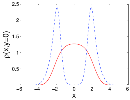
Figure 1: Column density $\rho(x,y)$ along $y=0$ as function of $x$. The red solid (blue dashed) curve is for ground state in the single harmonic trap without (with) a central gaussian barrier.

We first discuss the simplest case of two non-interacting BECs ($Q=0$ and $D=0$), assuming the dipolar interaction can be tuned to zero pfau6 . In Fig. 2, we show our numerical results of linear density $\rho(x,t)$ as function of time $t$ for the relative phase $\phi=0$. $\rho(x,t)$ is obtained by integrating along both the $y$- and $z$-axis, i.e. $\rho(x,t)=\int\int dydz|\psi({\bf r},t)|^{2}$. At the initial time, the two BECs are well separated. After the barrier is turned off, the two BECs start to collide with each other. As a consequence, we can see an interference pattern between them. The interference pattern disappears when the two BECs pass through each other. The two BECs are then reflected by the harmonic trap and ready for the collision in the next cycle. Such a necklace pattern of $\rho(x,t)$ is expected to keep repeating itself, with only a few cycles are selectively shown in Fig. 2. Because the two BECs are non-interacting, this pattern persists and collapse will not take place.

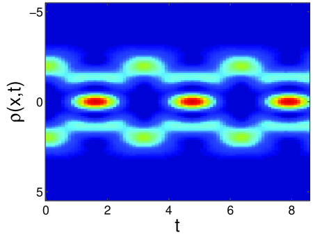
Figure 2: Linear density distribution $\rho(x)$ as function of time $t$ for two non-interacting condensates with $\phi=0$. Blue (red) stands for the minimum (maximum) density.

Now we present the numerical results for dipolar condensates ($Q=0$ and $D=16.5$). Firstly, the density distribution differs significantly from that in the non-interacting case. Secondly and more importantly, we observe the collapse of the two BECs which is absent in the non-interacting case. Our numerical results for relative phase $\phi=0$ are presented in Figs. 3-5. In Fig. 3, we show the density distributions $\rho(x,t)$ and $\rho(x,y,t)$ as function of time $t$. From the upper figure in Fig. 3, we can see that the two dipolar BECs behave similarly to non-interacting BECs: they collide with each other, interfere, and are reflected by the harmonic trap. However, the differences between them still merit some discussions here. One difference is that the period of the first cycle is about 4.5 which is larger than that of non-interacting BECs ($\sim 3$). This slowed motion is reminiscent of the damping effect for non-dipolar condensates ($Q\neq 0$ and $D=0$) where the interaction causes complex flow patterns acting as a damping force scott ; bo1 ; bo2 . Here we also find complex flow patterns for the dipolar interaction. Selected plots for the probability current $\vec{J}={\hbar\over m}{\rm Im}[\psi^{*}(x,y,z,t)\nabla\psi(x,y,z,t)]$ ($``\rm{Im}"$ denotes the imaginary part) are shown in Fig. 4. The upper row of Fig. 4 is for non-interacting condensates where the flow lines are all along the $x$-axis. However, in the lower row of Fig. 4 as for interacting condensates, we can see flow lines bent by the interaction. As a result of the damped motion, roughly 5 interference fringes can be seen, cf only 3 interference fringes can be seen for the non-interacting case. Another difference is the increased density in the central region at the final time ($t\sim 6.5$) which leads to the collapse effect. Since the total atom number is much lower than the critical atom number, this collapse is purely seeded by local density fluctuations. In this case, the interference is responsible for the enhancement in the density distribution. Although the dipolar interaction is cylindrically symmetric, the existence of the initial central barrier breaks this symmetry. As a result, the density distribution will develop an anisotropic pattern in the transverse plane. This cannot be seen from the linear density but instead can be seen from the column density $\rho(x,y,t)$. In the lower part of Fig. 3, we show 6 time snapshots (a-f) for $\rho(x,y,t)$ whose times are also marked on the horizontal axis of the upper figure. The density patterns in Figs. 3(a)-(d) clearly show a cycle of collision. We can see that, due to the dipolar interaction, the density pattern of Fig. 3(d) is not the same as that of Fig. 3(a). At a later time $t\sim 5.6$ (Fig. 3(e)), the density also exhibits a distribution along the $y$-axis: the density is maximal in the central region and surrounded by 4 lobes. At the final time $t\sim 6.5$ (Fig. 3(f)) just before the collapse, the central density maximum evolves into a singularity and triggers the collapse. Note that this singularity is purely artificial since GPE cannot handle the post-collapse dynamics. However, the GPE can still provide an accurate prediction of the onset of this collapse. Therefore, we still choose to present Fig. 3(f) to demonstrate the singular density profile. From the definition of $D$, where $N/a_{ho}^{3}$ is just the averaged density, it is perhaps not surprising that the local density fluctuations may induce collapse even though the total atom number is far below the critical atom number. What is somewhat more interesting is that the collapse does not happen during the first cycle of collision ($t\sim 0-4.5$) but only at a later time ($t\sim 6.5$). This is different from the previous study for the case of attractive s-wave scattering where the collapse happens during the first cycle of collision adams1 . In our case, it takes longer time for the anisotropic dipolar interaction to build up the local density fluctuation and eventually singularity.

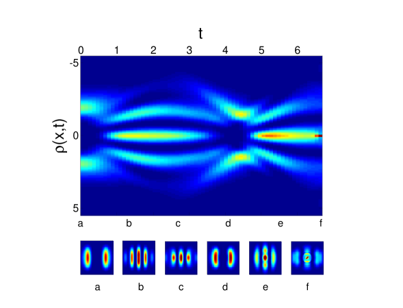
Figure 3: Upper figure: linear density distribution $\rho(x)$ as function of time $t$ for $\phi=0$. Lower figure: column density $\rho(x,y,t)$ as 6 different times labelled by (a)-(f). Field of view in each subplot is $(x,y)=[-3.5,3.5]\times[-3.5,3.5]$. In both figures, blue (red) stands for the minimum (maximum) density. However, the colormap of the upper figure is different from that of the lower figure and is adjusted for better visual effect.

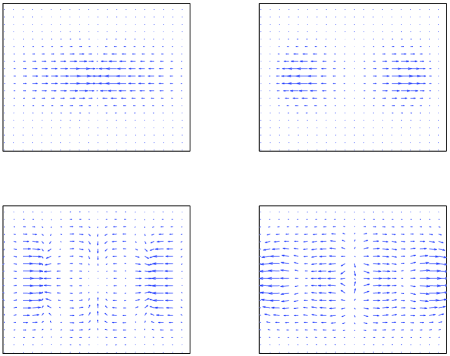
Figure 4: Probability current $J$ for $\phi=0$ at $t=1.43$ (left) and $t=2.86$ (right). The upper (low) row is for the non-interacting (dipolar) case. Field of view in each subplot is $(x,y)=[-3,3]\times[-3,3]$.

To track this collapse more quantitively, we show the energy per particle $E$ and the maximal density $\rho_{\rm max}$ as function of time $t$ in Fig. 5. $\rho_{\rm max}\equiv{\rm max}_{\{\bf r\}}|\psi({\bf r})|^{2}$ at each time step. The heating effect arising from the sudden removal of the barrier potential is negligible as the energy variation at the initial stage is about $0.5\hbar\omega_{\perp}/k_{B}\sim$ nK, so the description using GPE is still a good approximation. It is clear from Fig. 5 that the collapse is signaled by a sudden drop (increase) in $E$ ($\rho_{\rm max}$) due to the singularity developed in the condensate density. Here we are only interested in the onset of this collapse. Although the collapse dynamics afterwards are also interesting, a similar scenario of collapse has already been experimentally observed and discussed in detail in Ref. pfau4 and will not be discussed in this paper.

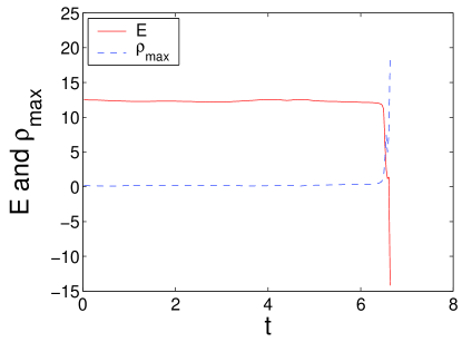
Figure 5: Energy per particle $E$ (red solid) and the maximal density $\rho_{\rm max}$ (blue dashed) as function of time $t$ $\phi=0$.

For other choices of $\phi$, we also observe the collapse effect. For example, in Fig. 6, we show $\rho(x,t)$ as function of time $t$ for $\phi=\pi$. We find that the period of the first cycle is close to that of $\phi=0$. Since the condensates are always in a phase of $\pi$, the two BECs never pass through each other. It seems as if they just collide and are bounced back from each other. However, we still observe strong density fluctuations and the induced collapse at $t\sim 8.7$. In this case, the density maximum is not in the center, rather it is found at two different locations at the same time. The complete dependence of the collapse time $t_{c}$ on $\phi$ is shown in Fig. 7. $t_{c}$ is defined as the time when $|1-E(t_{c})t_{c}/\int_{0}^{t_{c}}E(t)dt|=\delta$ and we choose $\delta=5\%$ here. Although a purely empirical definition, $t_{c}$ does capture the onset of the energy variation due to the diverging density profile. We find that a moderate change in $\delta$ does not change our conclusion qualitatively. The overall trend of the curve is that $t_{c}$ increases as $\phi$ increases. This can be explained as follows. For small $\phi\sim 0$, the collision behaves as “attractive” and the maximal density is likely to be found in the trap center resulting in a enhanced density. While for large $\phi\sim\pi$, the collision behaves as “repulsive” and the density maximum is likely to be located off the trap center resulting in a reduced density. In other words, it takes longer time to accumulate high enough density for larger $\phi$.

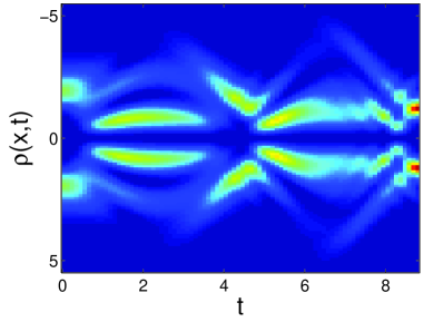
Figure 6: Linear density distribution $\rho(x)$ as function of time $t$ for $\phi=\pi$. Blue (red) stands for the minimum (maximum) density.

IV conclusion

In conclusion, we have studied the collision of two Bose-Einstein condensates with pure dipolar interaction. A stationary dipolar condensate is known to be stable when the atom number is below a critical value. However, we find that, even though the total atom number is just a fraction of the critical value, during the collision of two condensates, the local density fluctuations can still induce the collapse. To demonstrate this, we have performed full three-dimensional numerical simulations for typical experimental parameters. We present density distributions as function of time for different relative phases and compare them with those of two non-interacting condensates. We find that the dipolar interaction modifies the density profiles significantly. In addition, we show the collapse time as function of the relative phase between the two condensates. It turns out that a larger relative phase tends to increase the collapse time. We hope our study can be helpful to the ongoing experiments with degenerate dipolar gases.

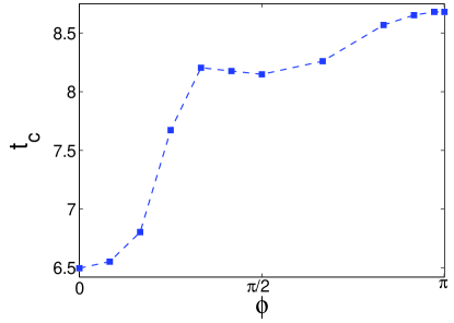
Figure 7: Collapse time $t_{c}$ as function of the relative phase $\phi$. Data points with blue square are numerical results. Dashed line is a guide to eyes.

This work is supported in part by an NSF grant to Auburn University. Computational work was carried out at the National Energy Research Scientific Computing Center in Oakland, California.

References

- (1) A. Griesmaier, J. Werner, S. Hensler, J. Stuhler, and T. Pfau, Phys. Rev. Lett. 94, 160401 (2005).
- (2) Krzysztof Góral, Kazimierz Rzaz̧ewski, and Tilman Pfau, Phys. Rev. A 61, 051601 (2000).
- (3) S. Giovanazzi, A. Görlitz, and T. Pfau, J. Opt. B: Quantum Semiclass. Opt. 5, S208 (2003).
- (4) J. Stuhler, A. Griesmaier, T. Koch, M. Fattori, S. Giovanazzi, P. Pedri, L. Santos and T. Pfau, Phys. Rev. Lett. 95, 150406 (2005); S. Giovanazzi, P. Pedri, L. Santos, A. Griesmaier, M. Fattori, T. Koch, J. Stuhler, and T. Pfau Phys. Rev. A 74, 013621 (2006).
- (5) O. Dutta and P. Meystre, Phys. Rev. A 75, 053604 (2007).
- (6) T. Lahaye, T. Koch, B. Fröhlich, M. Fattori, J. Metz, A. Griesmaier, S. Giovanazzi, T. Pfau, Nature 448, 672 (2007).
- (7) S. Ronen, D. C. E. Bortolotti, and J. L. Bohn, Phys. Rev. Lett. 98, 030406 (2007).
- (8) T. Lahaye, J. Metz, B. Fröhlich, T. Koch, M. Meister, A. Griesmaier, T. Pfau, H. Saito, Y. Kawaguchi, and M. Ueda, Phys. Rev. Lett. 101, 080401 (2008).
- (9) J. Metz, T. Lahaye, B. Fröhlich, A. Griesmaier, T. Pfau, H. Saito, Y. Kawaguchi, and M. Ueda, New J. Phys. 11, 055032 (2009).
- (10) S. Yi and L. You, Phys. Rev. A 66, 013607 (2002).
- (11) L. Santos, G. V. Shlyapnikov, and M. Lewenstein, Phys. Rev. Lett. 90, 250403 (2003).
- (12) D. H. J. O Dell, S. Giovanazzi, and C. Eberlein, Phys. Rev. Lett. 92, 250401 (2004).
- (13) S. Ronen, D. C. E. Bortolotti, and J. L. Bohn, Phys. Rev. A 74, 013623 (2006).
- (14) S. Giovanazzi, L. Santos and T. Pfau, Phys. Rev. A 75, 015604 (2007).
- (15) C. Ticknor, N. G. Parker, A. Melatos, S. L. Cornish, D. H. J. O’Dell, and A. M. Martin, Phys. Rev. A 78, 061607(R) (2008).
- (16) N. G. Parker, C. Ticknor, A. M. Martin, and D. H. J. O’Dell, Phys. Rev. A 79, 013617 (2009).
- (17) J. L. Bohn, R. M. Wilson and S. Ronen, Laser Physics 19, 547 (2009).
- (18) N. G. Parker, A. M. Martin, S. L. Cornish and C. S. Adams, J. Phys. B: At. Mol. Opt. Phys. 41, 045303 (2008).
- (19) M. R. Andrews, C. G. Townsend, H.-J. Miesner, D. S. Durfee, D. M. Kurn, W. Ketterle, Science 275, 637 (1997).
- (20) S. Giovanazzi, A. Görlitz, and T. Pfau, Phys. Rev. Lett. 89, 130401 (2002).
- (21) R. G. Scott, A. M. Martin, S. Bujkiewicz, T. M. Fromhold, N. Malossi, O. Morsch, M. Cristiani, and E. Arimondo, Phys. Rev. A 69, 033605 (2004).
- (22) B. Sun, M. S. Pindzola, and L. You, Phys. Rev. A 79, 033608 (2009).
- (23) B. Sun and M. S. Pindzola, to appear in Journal of Physics B, (2009).