Spontaneous Symmetry Breaking in General Relativity.
Brane World Concept.

Abstract

Gravitational properties of a hedge-hog type topological defect in two extra dimensions are considered in General Relativity employing a vector as the order parameter. The developed macroscopic theory of phase transitions with spontaneous symmetry breaking is applied to the analysis of possible ”thick” brane structures. The previous considerations were done using the order parameter in the form of a multiplet in a target space of scalar fields. The difference of these two approaches is analyzed and demonstrated in detail.

There are two different symmetries of regular solutions of Einstein equations for a hedgehog type vector order parameter. Both solutions are analyzed in parallel analytically and numerically. Regular configurations in cases of vector order parameter have one more free parameter in comparison with the scalar multiplet solutions.

It is shown that the existence of a negative cosmological constant is sufficient for the spontaneous symmetry breaking of the initially plain bulk.

Regular configurations have a growing gravitational potential and are able to trap the matter to the brane. Among others there are solutions with the gravitational potential having several points of minimum. Identical in the uniform bulk spin-less particles, being trapped within separate points of minimum, acquire different masses and appear to an observer within the brane as different particles with integer spins.

I Introduction

The theories of brane world and multidimensional gravity are widely discussed in the literature. They continue numerous attempts to find the origin of enormous hierarchy of energy and mass scales observed in nature, to explain the dark matter and dark energy effects, and other long-standing problems in physics. One can find a great variety of separate brane-world models in the literature: thin and thick branes in five and more dimensions, flat or curved branes and bulk, different mechanisms of brane formation, etc.

From my point of view the most natural approach is to consider the appearance of a distinguished hyper-surface in the space-time manifold as a result of a phase transition with spontaneous symmetry breaking in the early phase of the Universe formation. The macroscopic Landau theory of phase transitions with spontaneous symmetry breaking allows to consider the brane world concept self-consistently, even without the knowledge of the nature of physical vacuum. It is reasonable to regard the brane world as a topological defect, which inevitably appears as a result of a phase transition with spontaneous symmetry breaking.

The properties of topological defects (strings, monopoles, …) are generally described in general relativity with the aid of a multiplet of scalar fields forming a hedgehog-type configuration in extra dimensions (see Bron 1 and references there in). The scalar multiplet plays the role of the order parameter. The hedgehog-type multiplet configuration is proportional to a unit vector in the Euclidean target space of scalar fields. Though this model is self-consistent, it is not the direct way for generalization of a plane monopole to the curved space-time.

In a flat space-time there is no difference between a vector and a hedgehog-type multiplet of scalar fields. On the contrary, in a curved space-time scalar multiplets and real vectors are transformed differently. For this reason in general relativity the two approaches (a multiplet of scalar fields and a vector order parameter) give different results which are worth to be compared. It is the subject of this paper. A priory it seems more difficult to deal with a vector order parameter, and, probably, it is the reason why I couldn’t find in the literature any papers considering phase transitions with a hedgehog-type vector order parameter in general relativity.

The spontaneous symmetry breaking with a hedgehog-type vector order parameter in application to the brane world with two extra dimensions is considered in this paper. General formulae (section II) are applied to the analytical (section III) and numerical (IV) analysis of gravitational properties of global strings in two extra dimensions. The results are summarized in section V.

II General approach

II.1 Lagrangian

The order parameter enters the Lagrangian via scalar bilinear combinations of its covariant derivatives and via a scalar potential $V$ allowing the spontaneous symmetry breaking. If $\phi_{I}$ is a vector order parameter, then $V$ should  be  a function of the scalar $\phi^{K}\phi_{K}=g^{IK}\phi_{I}\phi_{K},$ and a bilinear combination of the derivatives is a tensor

$$S_{IKLM}=\phi_{I;K}\phi_{L;M}.$$

Index _;K is used as usual for covariant derivatives. There are three ways to simplify $S_{IKLM}$ into scalars, so the most general form of the scalar $S,$ formed via contractions of $S_{IKLM},$ is

$$S=A\left(\phi_{;K}^{K}\right)^{2}+B\phi_{;K}^{L}\phi_{L}^{;K}+C\phi_{;K}^{M}\phi_{;M}^{K},$$ (1)

where $A,B,$ and $C$ are arbitrary constants. Different topological defects can be classified by these parameters. In curved space-time the scalar $S$ depends not only on the derivatives of the order parameter, but also on the derivatives of the metric tensor. This is the principle difference between a vector and a multiplet of scalar fields.

The general form of the Lagrangian determining gravitational properties of topological defects with a vector order parameter is

$$L\left(\phi_{I},g^{IK},\frac{\partial g_{IK}}{\partial x^{L}}\right)=L_{g}+L_{d},$$

where

$$L_{g}=\frac{R}{2\kappa^{2}},$$ (2)

$$L_{d}=A\left(\phi_{;K}^{K}\right)^{2}+B\phi_{;K}^{I}\phi_{I}^{;K}+C\phi_{;K}^{I}\phi_{;I}^{K}-V\left(\phi^{K}\phi_{K}\right).$$ (3)

$L_{g}$ is the Lagrangian of the gravitational field, $R$ is the scalar curvature of space-time, $\kappa^{2}$ is the (multidimensional) gravitational constant, and $L_{d}$ is the Lagrangian of a topological defect. Covariant derivation

$$\phi_{P;M}=\frac{\partial\phi_{P}}{\partial x^{M}}-\frac{1}{2}g^{LA}\left(\frac{\partial g_{AM}}{\partial x^{P}}+\frac{\partial g_{AP}}{\partial x^{M}}-\frac{\partial g_{MP}}{\partial x^{A}}\right)\phi_{L}$$ (4)

and razing of indexes $\phi^{K}=g^{IK}\phi_{I}$ contain $g^{IK}$ and $\frac{\partial g_{IK}}{\partial x^{L}},$ and for this reason it is convenient to consider the Lagrangian as a function of $\phi_{I},$ $g^{IK},$ and $\frac{\partial g_{IK}}{\partial x^{L}}$.

II.2 Energy-momentum tensor

Varying the Lagrangian $L_{d}$ $\left(\ref{Ldef}\right)$ with respect to $\delta g^{IK}$ and having in mind that

$$\delta g_{IK}=-g_{KM}g_{IN}\delta g^{NM},$$ (5)

we get the following expression for the energy-momentum tensor :

$$\begin{array}[]{c}T_{IK}=\frac{2}{\sqrt{-g}}\left[\frac{\partial\sqrt{-g}L_{d}}{\partial g^{IK}}+g_{QK}g_{PI}\frac{\partial}{\partial x^{L}}\left(\sqrt{-g}\frac{\partial L_{d}}{\partial\frac{\partial g_{PQ}}{\partial x^{L}}}\right)\right]\end{array}$$ (6)

In the case of the vector order parameter the symmetry breaking potential $V\left(\phi^{K}\phi_{K}\right)=V\left(g^{IK}\phi_{I}\phi_{K}\right)$ also takes part in the variation with respect to $\delta g^{IK}$.

In what follows we apply this approach to the particular topological defect, namely the global string in two extra dimensions.

III Global string in extra dimensions

In my previous papers with Bronnikov (see Bron 1 and references there in) we considered global monopoles and strings as topological defects with the order parameter in the form of a hedge-hock type multiplet of scalar fields in some flat target space. The aim of this paper is to describe these defects using vector order parameter and compare the results.

III.1 Metric

The direction of the vector specifies one coordinate, and in the most simple case the system is uniform and isotropic with respect to all other coordinates. In our recent paper Bron 1 we presented the detailed properties of global strings in two extra dimensions. For this reason I consider below a topological defect in the space-time with two extra dimensions. The order parameter is a space-like vector $(g^{IK}\phi_{I}\phi_{K}<0)$ directed normally from the brane hypersurface and depending on the only one specific coordinate, namely – the distance from the brane. The whole $\left(D=d_{0}+2\right)$-dimensional space-time has the structure M${}^{d_{0}}\times$ R${}^{1}\times$ $\Phi^{1}$ and the metric

$$ds^{2}=e^{2\gamma\left(l\right)}\eta_{\mu\nu}dx^{\mu}dx^{\nu}-\left(dl^{2}+e^{2\beta\left(l\right)}d\varphi^{2}\right),$$ (7)

where $\eta_{\mu\nu}=$ diag $\left(1,-1,...,-1\right)$ is the $d_{0}$-dimensional Minkovsky brane metric $(d_{0}>1,$ we set $d_{0}=4$ in computations) , and $\varphi$ is the angular cylindrical coordinate in extra dimensions. $\gamma$ and $\beta$ are functions of the distinguished extradimensional coordinate $l$ – the distance from the center, i.e. from the brane. $e^{\beta\left(l\right)}=r\left(l\right)$ is the circular radius. Greek indices $\mu,\nu,..$ correspond to $d_{0}$-dimensional space-time on the brane, and $I,K,...$ – to all $D=d_{0}+2$ coordinates. The metric tensor $g_{IK}$ is diagonal, and its nonzero components are denoted as follows:

$$g_{IK}=\left\{\begin{array}[]{l}e^{2\gamma},\quad I=K=0,\\ -e^{2\gamma},\quad 0<I=K<d_{0},\\ -1,\quad I=K=d_{0},\\ -e^{2\beta},\quad I=K=\varphi.\end{array}\right.$$

The curvature of the metric on brane due to the matter is supposed to be much smaller than the curvature of the bulk caused by the brane formation.

III.2 Regularity conditions

If the influence of matter on brane is neglected, then there is no physical reason for singularities, and the selfconsistent structure of a topological defect should be regular. A necessary condition of regularity is finiteness of all invariants of the Riemann tensor of curvature. The nonzero components of the Riemann tensor are

$$\begin{array}[]{c}R_{\text{ \ \ }CD}^{AB}=\left\{\begin{array}[]{l}-\gamma^{\prime 2}\left(\delta_{C}^{A}\delta_{D}^{B}-\delta_{D}^{A}\delta_{C}^{B}\right),\quad A,B,C,D<d_{0},\\ -\beta^{\prime}\gamma^{\prime},\quad A=C=\varphi,\quad B,D<d_{0},\\ -\left(\gamma^{\prime\prime}+\gamma^{\prime 2}\right)\delta_{D}^{B},\quad A=C=d_{0},\quad B,D<d_{0},\\ -\left(\beta^{\prime\prime}+\beta^{\prime 2}\right),\quad A=C=d_{0},\quad B=D=\varphi.\end{array}\right.\end{array}$$ (8)

Here prime denotes $d/dl.$ One of the invariants of the Riemann tensor is the Kretchmann scalar $K=R_{\text{ \ \ }CD}^{AB}R_{\text{ \ \ }AB}^{CD}$ , which is the sum of all nonzero $R_{\text{ \ \ }CD}^{AB}$ squared. Hence all the nonzero components of the Riemann tensor, and namely

$$\gamma^{\prime},\ \ \gamma^{\prime\prime}+\gamma^{\prime 2},\ \ \beta^{\prime}\gamma^{\prime},\ \ \beta^{\prime\prime}+\beta^{\prime 2}$$ (9)

must be finite. The center $r=0$ is a singular point of the cylindrical coordinate system. The absence of curvature singularity in the center follows from the finiteness of the last term in $\left(\ref{Regul conditions}\right).$ Let

$$\beta^{\prime\prime}+\beta^{\prime 2}=c<\infty\text{\ \ \ at \ \ }l=0.$$ (10)

Integrating $\left(\ref{Bet''+Bet'^2=c}\right)$ in the vicinity of the center we have

$$\beta^{\prime}=\frac{1}{l}+\frac{1}{3}cl+O\left(l^{3}\right).$$ (11)

Relation $\left(\ref{Bet'=1/l+..}\right)$ ensures the correct $\left(=2\pi\right)$ circumference-to-radius ratio, or, equivalently, $dr^{2}=dl^{2}$ at $l\rightarrow 0.$ Finiteness of $\beta^{\prime}\gamma^{\prime}$ at $l=0$ is fulfilled if

$$\gamma^{\prime}=O\left(l\right)\text{\ \ \ or \ \ smaller \ \ at \ \ }l\rightarrow 0.$$ (12)

III.3 Vector order parameter

Our aim is to consider the order parameter as a vector in extra dimensions directed normally from the Minkovsky hypersurface. In the cylindrical coordinate system of extra dimensions the only nonzero component of the vector order parameter is

$$\phi_{d_{0}}\equiv\phi.$$ (13)

In the space-time with the metric $\left(\ref{metric}\right)$ the covariant derivative

$$\phi_{I;K}=\delta_{I}^{d_{0}}\delta_{K}^{d_{0}}\phi^{\prime}-\frac{1}{2}\delta_{IK}g^{II}g_{II}^{\prime}\phi$$ (14)

is a symmetric tensor: $\phi_{I\text{ };K}=\phi_{K\text{ };I}.$ For this reason $\phi_{\text{ };K}^{I}\phi_{I\text{ }}^{\text{ };K}=\phi_{\text{ };K}^{I}\phi_{\text{ };I}^{K}$ , and without loss of generality we set $C=0.$ The Lagrangian $\left(\ref{Ldef}\right)$ takes the form

$$\begin{array}[]{c}L_{d}=A\left(\phi^{\prime}+\frac{1}{2}\phi\sum_{K}g^{KK}g_{KK}^{\prime}\right)^{2}+B\left(\phi^{\prime 2}+\frac{1}{4}\phi^{2}\sum_{L}\left(g^{LL}g_{LL}^{\prime}\right)^{2}\right)-V\left(-\phi^{2}\right).\end{array}$$ (15)

It contains only two arbitrary constants $A$ and $B.$ In $\left(\ref{L_d=...}\right)$ we set $g^{d_{0}d_{0}}=-1$ in accordance with $\left(\ref{metric}\right).$ However one should keep in mind that $\left(\ref{L_d=...}\right)$ cannot be used in $\left(\ref{Tik}\right).$ To derive the energy-momentum tensor $\left(\ref{Tik}\right)$ one should use the Lagrangian $\left(\ref{Ldef}\right),$ and set $g^{d_{0}d_{0}}=-1,$ $\left(g^{d_{0}d_{0}}\right)^{\prime}=0$ after differentiation. Nevertheless, the field equation can be derived using $\left(\ref{L_d=...}\right)$ in the general formula

$$\frac{1}{\sqrt{-g}}\left(\frac{\partial\sqrt{-g}L_{d}}{\partial\phi^{\prime}}\right)^{\prime}-\frac{\partial L_{d}}{\partial\phi}=0.$$ (16)

In the space-time with metric $\left(\ref{metric}\right)$ the sums in $\left(\ref{L_d=...}\right)$ are

$$\begin{array}[]{c}S_{n}=\frac{1}{2^{n}}\sum_{K}\left(g^{KK}g_{KK}^{\prime}\right)^{n}=d_{0}\gamma^{\prime n}+\beta^{\prime n},\quad n=1,2,...\text{ .}\end{array}$$ (17)

and the determinant of the metric tensor is

$$g=\left(-1\right)^{D-1}e^{2\left(d_{0}\gamma+\beta\right)}.$$ (18)

We consider below the two cases, case A ($A\neq 0,$ $B=0$) and case B ($B\neq 0,$ $A=0$), in comparison, but separately.

III.4 Field equations

Substituting $\left(\ref{L_d=...}\right)$ into $\left(\ref{(dL_d/dFi')'-dL_d/dFi=0}\right)$ we get the field equations in the case of vector order parameter.

Case A
In case $A=\frac{1}{2},$ $B=0$ we get

$$\left(\phi^{\prime}+S_{1}\phi\right)^{\prime}+\frac{\partial V}{\partial\phi}=0.$$ (19)

Case B
In the case $B=\frac{1}{2},$ $A=0$ the substitution results in

$$\phi^{\prime\prime}+S_{1}\phi^{\prime}-S_{2}\phi+\frac{\partial V}{\partial\phi}=0.$$ (20)

$S_{1}$ and $S_{2}$ are defined in (17).

Case of scalar multiplet
In the case of the multiplet of scalar fields we had Bron 1 :

$$\phi^{\prime\prime}+S_{1}\phi^{\prime}-\phi e^{-2\beta}+\frac{\partial V}{\partial\phi}=0.$$ (21)

Unlike (21), the field equations (19) and (20) do not depend directly on $\beta$ (and thus on the circular radius $r=\ln\beta)$. The case A field equation (19) includes second derivatives of the metric tensor. In the flat space-time $\gamma^{\prime}=0,$ $\beta^{\prime}=\frac{1}{l},$ $\beta^{\prime\prime}=-\frac{1}{l^{2}},e^{-2\beta}=\frac{1}{l^{2}},$  and all three field equations (19), (20), and (21) reduce to

$$\phi^{\prime\prime}+\frac{1}{l}\phi^{\prime}-\frac{1}{l^{2}}\phi+\frac{\partial V}{\partial\phi}=0.$$ (22)

III.5 Energy-momentum tensor

The energy-momentum tensor $\left(\ref{Tik}\right)$ inevitably contains second derivatives. However, in case A the second derivatives can be excluded with the aid of the field equation $\left(\ref{Field equationA}\right)$. In case B the second derivatives cannot be excluded from the energy-momentum tensor. The final result of rather wearing derivations is:

Case A

$$\begin{array}[]{c}T_{I}^{K}=\frac{1}{2}\delta_{I}^{K}\left(\phi^{\prime}+S_{1}\phi\right)^{2}+\delta_{I}^{K}V+\left(\delta_{I}^{d_{0}}\delta_{d_{0}}^{K}-\delta_{I}^{K}\right)\frac{\partial V}{\partial\phi}\phi\end{array}$$ (23)

Case B

$$\begin{array}[]{l}T_{I<d_{0}}^{K}=\delta_{I}^{K}\left[\frac{1}{\sqrt{-g}}\left(\sqrt{-g}\gamma^{\prime}\right)^{\prime}\phi^{2}+\gamma^{\prime}\left(\phi^{2}\right)^{\prime}-\left(\frac{1}{2}\phi^{\prime 2}+\frac{1}{2}S_{2}\phi^{2}\right)+V\right]\\ T_{d_{0}}^{d_{0}}=\frac{1}{2}\left(\phi^{\prime 2}+S_{2}\phi^{2}\right)+V\\ T_{I>d_{0}}^{K}=\delta_{I}^{K}\left[\frac{1}{\sqrt{-g}}\left(\sqrt{-g}\beta^{\prime}\right)^{\prime}\phi^{2}+\beta^{\prime}\left(\phi^{2}\right)^{\prime}-\left(\frac{1}{2}\phi^{\prime 2}+\frac{1}{2}S_{2}\phi^{2}\right)+V\right]\end{array}$$ (24)

Unlike the scalar multiplet case, the energy-momentum tensor $\left(\ref{T ik=1/2Delta^K_I...A}\right)$ contains not only the potential $V,$ but also its derivative $\frac{\partial V}{\partial\phi}$.

Correctness of $\left(\ref{T ik=1/2Delta^K_I...A}\right)$ and $\left(\ref{T ik=1/2Delta^K_I...B}\right)$ is checked by the derivation of the covariant divergence $T_{I\text{ };K}^{K}$ (actually $T_{d_{0}\text{ };K}^{K})$. Again, with the aid of field equations $\left(\ref{Field equationA}\right)$ and $\left(\ref{Field equationB}\right)$ we confirm that

$$T_{d_{0}\text{ };K}^{K}=0.$$

III.6 Einstein equations

The same way as in Bron 1 we use the Einstein equations in the form

$$R_{I}^{K}=\kappa^{2}\widetilde{T}_{I}^{K},$$

where $R_{I}^{K}$ is the Ricci tensor,

$$R_{I}^{K}=\left\{\begin{array}[]{c}\delta_{I}^{K}\left(\gamma^{\prime\prime}+\gamma^{\prime}S_{1}\right),\quad I<d_{0}\\ \delta_{d_{0}}^{K}\left(S_{1}^{\prime}+S_{2}\right),\quad I=d_{0}\\ \delta_{\varphi}^{K}\left(\beta^{\prime\prime}+S_{1}\beta^{\prime}\right),\quad I=\varphi\end{array}\right.$$

and

$$\begin{array}[]{c}\widetilde{T}_{I}^{K}=T_{I}^{K}-\frac{1}{d_{0}}\delta_{I}^{K}T.\end{array}$$

In both cases A and B the sets of Einstein equations consist of three first order equations with respect to $\gamma^{\prime},$ $\beta^{\prime},$ and $\phi$ :

Case A

$$\begin{array}[]{c}\gamma^{\prime\prime}+S_{1}\gamma^{\prime}=\kappa^{2}\left[-\frac{1}{d_{0}}\left(\phi^{\prime}+S_{1}\phi\right)^{2}-\frac{2V}{d_{0}}+\frac{1}{d_{0}}\frac{\partial V}{\partial\phi}\phi\right]\end{array}$$ (27)

$$\begin{array}[]{c}S_{1}^{\prime}+S_{2}=\kappa^{2}\left[-\frac{1}{d_{0}}\left(\phi^{\prime}+S_{1}\phi\right)^{2}-\frac{2V}{d_{0}}+\left(1+\frac{1}{d_{0}}\right)\frac{\partial V}{\partial\phi}\phi\right]\end{array}$$ (29)

$$\begin{array}[]{c}\beta^{\prime\prime}+S_{1}\beta^{\prime}=\kappa^{2}\left[-\frac{1}{d_{0}}\left(\phi^{\prime}+S_{1}\phi\right)^{2}-\frac{2V}{d_{0}}+\frac{1}{d_{0}}\frac{\partial V}{\partial\phi}\phi\right]\end{array}$$ (31)

Case B

$$\begin{array}[]{c}\gamma^{\prime\prime}+S_{1}\gamma^{\prime}=\kappa^{2}\left[S_{1}\gamma^{\prime}\phi^{2}+\left(\gamma^{\prime}\phi^{2}\right)^{\prime}-\frac{1}{d_{0}}S_{1}^{2}\phi^{2}-\frac{1}{d_{0}}\left(S_{1}\phi^{2}\right)^{\prime}-\frac{2}{d_{0}}V\right]\end{array}$$ (33)

$$\begin{array}[]{c}S_{1}^{\prime}+S_{2}=\kappa^{2}\left[\phi^{\prime 2}+S_{2}\phi^{2}-\frac{1}{d_{0}}S_{1}^{2}\phi^{2}-\frac{1}{d_{0}}\left(S_{1}\phi^{2}\right)^{\prime}-\frac{2}{d_{0}}V\right]\end{array}$$ (35)

$$\begin{array}[]{c}\beta^{\prime\prime}+S_{1}\beta^{\prime}=\kappa^{2}\left[S_{1}\beta^{\prime}\phi^{2}+\left(\beta^{\prime}\phi^{2}\right)^{\prime}-\frac{1}{d_{0}}S_{1}^{2}\phi^{2}-\frac{1}{d_{0}}\left(S_{1}\phi^{2}\right)^{\prime}-\frac{2}{d_{0}}V\right]\end{array}$$ (37)

Metric functions $\gamma$ and $\beta$ do not enter the equations $\left(\ref{Gamma''+...A}-\ref{Beta''+...B}\right)$ directly, only via the derivatives. In the case of a scalar multiplet order parameter, see eq.$\left(14-16\right)$ in Bron 1 , $\beta$ enters the Einstein equations directly, and the system of equations is of the fourth order. It is also worth to mention that the right hand sides of first and third equations coincide in case A, and have a similar structure in case B. This symmetry reflects the fact that the coordinates $x^{I}$ with $I<d_{0}$ and $I=\varphi$ are cyclic variables.

The field equations $\left(\ref{Field equationA}\right)$ and $\left(\ref{Field equationB}\right)$ are not independent. They are consequences of the Einstein equations due to the Bianchi identities.

III.7 First integrals

Excluding the second derivatives $\gamma^{\prime\prime}$ and $\beta^{\prime\prime}$ in the sets $\left(\ref{Gamma''+...A}-\ref{Beta''+...A}\right)$ and $\left(\ref{Gamma''+...B}-\ref{Beta''+...B}\right),$ we get the relations

Case A

$$\begin{array}[]{c}S_{1}^{2}-S_{2}=-\kappa^{2}\left[\left(\phi^{\prime}+S_{1}\phi\right)^{2}+2V\right],\end{array}$$ (38)

Case B

$$\begin{array}[]{c}S_{2}\left(1-\kappa^{2}\phi^{2}\right)=\kappa^{2}\phi^{\prime 2}+2\kappa^{2}V+S_{1}^{2},\end{array}$$ (39)

which can be considered as first integrals of the systems $\left(\ref{Gamma''+...A}-\ref{Beta''+...A}\right)$ and $\left(\ref{Gamma''+...B}-\ref{Beta''+...B}\right).$

III.8 Further simplification

The equations $\left(\ref{Gamma''+...A}\right)$ and $\left(\ref{Beta''+...A}\right),$ as well as the equations $\left(\ref{Gamma''+...B}\right)$ and $\left(\ref{Beta''+...B}\right),$ have similar structures. Extracting in both cases one from the other, we get the equations

Case A

$$\left(\gamma^{\prime}-\beta^{\prime}\right)^{\prime}+\left(\gamma^{\prime}-\beta^{\prime}\right)S_{1}=0,$$ (40)

Case B

$$\left[\left(\gamma^{\prime}-\beta^{\prime}\right)\left(1-\kappa^{2}\phi^{2}\right)\right]^{\prime}+\left(\gamma^{\prime}-\beta^{\prime}\right)\left(1-\kappa^{2}\phi^{2}\right)S_{1}=0.$$ (41)

$\left(\ref{(Gamma'-Beta')'+...A}\right)$ can be used instead of one of the equations $\left(\ref{Gamma''+...A}\right)$ or $\left(\ref{Beta''+...A}\right)$ and, respectively, $\left(\ref{(Gamma'-Beta')'+...B}\right)$ – instead of $\left(\ref{Gamma''+...B}\right)$ or $\left(\ref{Beta''+...B}\right)$ .

With the aid of the relations $\left(\ref{First integralA}\right)$,$\left(\ref{(Gamma'-Beta')'+...A}\right)$ and $\left(\ref{First integralB}\right)$,$\left(\ref{(Gamma'-Beta')'+...B}\right)$ the complete sets of equations can be reduced to more simple forms. Introducing new functions

$$U=\gamma^{\prime}-\beta^{\prime},\text{ \ }Z=\phi^{\prime}+S_{1}\phi,\text{ \ }\psi=\phi^{\prime},$$ (42)

and having in mind that functions $\beta^{\prime},$ $\gamma^{\prime},$ and their combination $S_{2}=d_{0}\gamma^{\prime 2}+\beta^{\prime 2}$ $\left(\ref{Sums}\right)$ are expressed via $U$ and $S_{1}$ as follows:

$$\gamma^{\prime}=\frac{U+S_{1}}{d_{0}+1}\qquad\beta^{\prime}=\frac{S_{1}-d_{0}U}{d_{0}+1}\qquad S_{2}=\frac{d_{0}U^{2}+S_{1}^{2}}{d_{0}+1},$$

we get the sets of four first order equations, solved against the derivatives:

Case A

$$\begin{array}[]{c}U^{\prime}=-US_{1}\\ S_{1}^{\prime}=\kappa^{2}\frac{d_{0}+1}{d_{0}}\frac{\partial V}{\partial\phi}\phi-U^{2}\\ \phi^{\prime}=Z-S_{1}\phi\\ Z^{\prime}=-\frac{\partial V}{\partial\phi}\end{array}$$ (43)

Case B

$$\begin{array}[]{c}\left[U\left(1-\kappa^{2}\phi^{2}\right)\right]^{\prime}+U\left(1-\kappa^{2}\phi^{2}\right)S_{1}=0\\ \left[S_{1}\left(1+\frac{\kappa^{2}\phi^{2}}{d_{0}}\right)\right]^{\prime}+S_{1}^{2}\left(1+\frac{\kappa^{2}\phi^{2}}{d_{0}}\right)+\frac{2\left(1+d_{0}\right)}{d_{0}}\kappa^{2}V=0\\ \phi^{\prime}=\psi\\ \psi^{\prime}+S_{1}\psi-\frac{d_{0}U^{2}+S_{1}^{2}}{d_{0}+1}\phi+\frac{\partial V}{\partial\phi}=0\end{array}$$ (44)

The sets $\left(\ref{Convenient setA}\right)$ and $\left(\ref{Convenient setB}\right)$ are most convenient for both analytical and numerical analysis.

III.9 General analysis of regular solutions

The sets $\left(\ref{Convenient setA}\right)$ and $\left(\ref{Convenient setB}\right)$ are invariant against adding arbitrary constants to $\gamma$ and $\beta.$ Without loss of generality we can set

$$\gamma\left(0\right)=0.$$ (45)

Requirement of regularity in the center dictates the condition $\left(\ref{Bet'=1/l+..}\right),$ and, if we do not consider configurations with angle deficit (or surplus), we have

$$r=e^{\beta}=l\ \text{\ at }\ l\rightarrow 0.$$ (46)

Integrating first equations in the sets $\left(\ref{Convenient setA}\right)$ and $\left(\ref{Convenient setB}\right)$ with boundary conditions $\left(\ref{Gamma(0)=0},\ref{r=l at l to 0}\right)$ we get:

Case A

$$\gamma^{\prime}-\beta^{\prime}=-e^{-\left(d_{0}\gamma+\beta\right)},$$ (47)

Case B

$$\gamma^{\prime}-\beta^{\prime}=-\frac{e^{-\left(d_{0}\gamma+\beta\right)}}{1-\kappa^{2}\phi^{2}}.$$ (48)

From $\left(\ref{G'-B'=-e^(d0G+B)A}\right)$ and $\left(\ref{G'-B'=-e^(d0G+B)B}\right)$ it follows that in both cases $\beta^{\prime}>\gamma^{\prime}$ everywhere. Within the regions of regularity $e^{-\left(d_{0}\gamma+\beta\right)}\rightarrow 0$ at $l\rightarrow\infty,$ and $\gamma_{\infty}^{\prime}$ coincides with $\beta_{\infty}^{\prime}.$

The denominator in $\left(\ref{G'-B'=-e^(d0G+B)B}\right)$ is the origin of an important difference between the cases A and B. In the symmetric (unbroken) state the order parameter $\phi=0,$ and $\phi^{\prime}=0$ everywhere. In the state with broken symmetry $\phi^{\prime}\neq 0$, but still $\phi=0$ at a point of maximum of the symmetry breaking potential $V(\phi)$, which is supposed to coincide with the center $l=0$. Requirement of regularity is fulfilled only if the denominator in $\left(\ref{G'-B'=-e^(d0G+B)B}\right)$ remains positive everywhere. It means that in case B the order parameter $\phi(l)$ can never exceed $\kappa^{-1}:$

$$\kappa^{2}\phi^{2}<1,\qquad\textrm{case B.}$$ (49)

Case A is free from such a restriction.

Recall that topological defects, formed as multiplets of scalar fields Bron 1 , are of three types. Integral curves can terminate with:

A) infinite circular radius $r\left(l\right)$ at $l\rightarrow\infty;$

B) finite circular radius $r_{\infty}=r\left(\infty\right)=const<\infty;$

C) second center $r=0$ at some finite $l=l_{c}.$

In the vector order parameter case the situation is different. Equations $\left(\ref{G'-B'=-e^(d0G+B)A}\right)$ and $\left(\ref{G'-B'=-e^(d0G+B)B}\right)$ allow to prove that regular configurations in both cases A and B can not terminate neither with a finite value of circular radius $r_{\infty}$ at $l\rightarrow\infty,$ nor in the second center.

Suppose, for instance in case A, that $r_{\infty}=const<\infty.$ Then $\beta^{\prime}(\infty)=0,$ and $\left(\ref{G'-B'=-e^(d0G+B)A}\right)$ reduces to $\gamma^{\prime}=-\frac{1}{r_{\infty}}e^{-d_{0}\gamma}$ at $l\rightarrow\infty.$ After integration we get

$$e^{d_{0}\gamma}=\frac{d_{0}}{r_{\infty}}\left(l_{0}-l\right),$$

$l_{0}$ is a constant of integration. The l.h.s. is obviously positive, while the r.h.s. becomes negative and infinitely large at $l\rightarrow\infty.$ Thus $r_{\infty}=const<\infty$ is impossible.

The second center is also impossible. In the vicinity of the second center the l.h.s. of $\left(\ref{G'-B'=-e^(d0G+B)A}\right)$ becomes large positive due to $-\beta^{\prime},\$and the r.h.s. remains negative.

We come to the conclusion that regular configurations of topological defects with the vector order parameter start at the center $l=0$ and always terminate at $l\rightarrow\infty$ with infinitely growing circular radius $r\left(l\right)\rightarrow\infty.$

It follows from the requirement of regularity $\left(\ref{Gamma'=O(l)}\right)$ that $\gamma^{\prime}$ $=\gamma_{0}^{\prime\prime}l$ at $l\rightarrow 0.$ From the first integrals $\left(\ref{First integralA}\right)$ and $\left(\ref{First integralB}\right)$ we find the relations between $\gamma_{0}^{\prime\prime},\phi_{0}^{\prime},$ and $V_{0}:$

Case A

$$\gamma_{0}^{\prime\prime}=-\frac{\kappa^{2}}{d_{0}}\left(2\phi_{0}^{\prime 2}+V_{0}\right),$$ (50)

Case B

$$\gamma_{0}^{\prime\prime}=-\frac{\kappa^{2}}{d_{0}}\left(\frac{1}{2}\phi_{0}^{\prime 2}+V_{0}\right),$$ (51)

where $V_{0}$ is the value of the symmetry breaking potential at the center $l=0.$ In both cases A and B, as well as in the case of scalar multiplet, the value $\phi_{0}^{\prime}=\phi^{\prime}\left(0\right)$ is not restricted by the equations. The difference is that in the scalar multiplet case $\phi_{0}^{\prime}$ becomes fixed unanimously by the requirement of regularity, while in both cases of vector order parameter

$\phi_{0}^{\prime}$ remains a free parameter.

III.10 Asymptotic behavior

Condition of regularity requires that $\gamma^{\prime}$ is finite everywhere. Within the area of regularity it tends to a fixed finite value $\gamma_{\infty}^{\prime}$ at $l\rightarrow\infty$. As soon as $r\left(l\right)\rightarrow\infty$ at $l\rightarrow\infty,$ we see from $\left(\ref{G'-B'=-e^(d0G+B)A}\right)$ and $\left(\ref{G'-B'=-e^(d0G+B)B}\right)$ that $\gamma^{\prime}-\beta^{\prime}\rightarrow 0$ in both cases A and B. Thus $\beta^{\prime}\left(\infty\right)=\gamma_{\infty}^{\prime}.$ The field $\phi\left(l\right)$ also tends to its finite value $\phi_{\infty}=\phi\left(\infty\right).$

Case A
From the field equation $\left(\ref{Field equationA}\right)$ it follows that $\frac{\partial V}{\partial\phi}\rightarrow 0$ at $l\rightarrow\infty,$ i.e. in the case A regular configurations terminate at an extremum of the potential $V\left(\phi\right)$. Let $V_{\infty}=V\left(\phi_{\infty}\right),$ $V^{\prime}\left(\phi_{\infty}\right)=0.$ From the first integral $\left(\ref{First integralA}\right)$ we find the limiting value $\gamma_{\infty}^{\prime}:$

$$\gamma_{\infty}^{\prime}=\sqrt{-\frac{2\kappa^{2}V_{\infty}}{\left(d_{0}+1\right)\left[d_{0}+\left(d_{0}+1\right)\kappa^{2}\phi_{\infty}^{2}\right]}}.$$ (52)

A necessary condition of existence of regular configurations of topological defects with the vector order parameter is $V_{\infty}<0.$

Case B
At $l\rightarrow\infty$ the second equation in $\left(\ref{Convenient setB}\right)$ reduces to

$$S_{1\infty}^{2}\left(1+\frac{\kappa^{2}\phi_{\infty}^{2}}{d_{0}}\right)+\frac{2\left(1+d_{0}\right)}{d_{0}}\kappa^{2}V_{\infty}=0.$$

We see that in this case also

$$V_{\infty}=V\left(\phi_{\infty}\right)<0.$$ (53)

The fourth equation in $\left(\ref{Convenient setB}\right)$ reduces to

$$-S_{1\infty}^{2}\frac{\phi_{\infty}}{d_{0}+1}+\frac{\partial V_{\infty}}{\partial\phi}=0,$$

and so

$$\frac{1}{2\phi_{\infty}}\frac{\partial V_{\infty}}{\partial\phi}\equiv\frac{\partial V_{\infty}}{\partial\phi^{2}}>0.$$ (54)

Here $V_{\infty}$ and$\ \frac{\partial V_{\infty}}{\partial\phi}$ are the values of the symmetry breaking potential and its derivative at $l\rightarrow\infty.$ Unlike the case A, in case B regular configurations terminate at a slope of the potential, and not at a point of extremum. Excluding $S_{1}^{2}$ we get the equation determining $\phi_{\infty}=\phi\left(\infty\right):$

$$\kappa^{2}V_{\infty}=-\left(d_{0}+\kappa^{2}\phi_{\infty}^{2}\right)\frac{\partial V_{\infty}}{\partial\phi^{2}}.$$ (55)

In view of $\ S_{1\infty}=\left(d_{0}+1\right)\gamma_{\infty}^{\prime},$ we find

$$\gamma_{\infty}^{\prime}=\sqrt{\frac{1}{\left(d_{0}+1\right)\phi_{\infty}}\frac{\partial V_{\infty}}{\partial\phi}}.$$ (56)

To find the behavior of $\phi\left(l\right)$ and $S_{1}\left(l\right)$ at large distances from the center we have to linearize the sets of equations $\left(\ref{Convenient setA}\right)$ and $\left(\ref{Convenient setB}\right)$ at $l\rightarrow\infty:$

$$\phi=\phi_{\infty}+\delta\phi,\text{ \ }S_{1}=\left(d_{0}+1\right)\gamma_{\infty}^{\prime}+\delta S_{1}.$$

Case A:

$$\begin{array}[]{c}\delta S_{1}^{\prime}=\kappa^{2}\frac{d_{0}+1}{d_{0}}V_{\infty}^{\prime\prime}\phi_{\infty}\delta\phi\\ \delta\phi^{\prime}=\delta Z-\left(d_{0}+1\right)\gamma_{\infty}^{\prime}\delta\phi-\phi_{\infty}\delta S_{1}\\ \delta Z^{\prime}=-V_{\infty}^{\prime\prime}\delta\phi\end{array}$$ (57)

Here primes denote derivatives $d/dl,$ $\left(\delta S_{1}^{\prime}=d(\delta S_{1})/dl,...\right),$ except $V_{\infty}^{\prime\prime}=\frac{\partial^{2}V}{\partial\phi^{2}}\left|{}_{\phi=\phi_{\infty}}\right..$  Excluding $\delta Z$ and $\delta S_{1},$ we get the second order linear homogeneous equation for $\delta\phi:$

$$\delta\phi^{\prime\prime}+\left(d_{0}+1\right)\gamma_{\infty}^{\prime}\delta\phi^{\prime}+\frac{2\kappa^{2}\left|V_{\infty}\right|V_{\infty}^{\prime\prime}}{d_{0}\left(d_{0}+1\right)\gamma_{\infty}^{\prime 2}}\delta\phi=0.$$

In case A the solution terminates at an extremum of $V(\phi)$. If the extremum of the potential is minimum, $\left(V_{\infty}^{\prime\prime}>0\right),$ the nontrivial solution vanishes at $l\rightarrow\infty:$

$$\delta\phi=Ae^{\lambda_{+}l}+Be^{\lambda_{-}l},$$ (58)

where $A$ and $B$ are constants of integration, and both eigenvalues

$$\lambda_{\pm}=-\frac{\left(d_{0}+1\right)\gamma_{\infty}^{\prime}}{2}\left(1\mp\sqrt{1-\frac{8\kappa^{2}\left|V_{\infty}\right|V_{\infty}^{\prime\prime}}{d_{0}\left(d_{0}+1\right)^{3}\gamma_{\infty}^{\prime 4}}}\right)$$ (59)

are either negative, or have negative real parts. Absence of growing solutions is the reason why $\phi_{0}^{\prime}$ remains a free parameter in the vector order parameter case.

In case A the asymptotic behavior of the field $\phi\left(l\right)$ far from the center is determined by two constant parameters of the symmetry breaking potential near its extremum, namely $V_{\infty}$ and $V_{\infty}^{\prime\prime}.$ If the extremum is minimum, $V_{\infty}^{\prime\prime}>0$, then the expression under the root can be both positive and negative. So $\phi\left(l\right)$ can tend to $\phi_{\infty}$ either smoothly, or with oscillations. In the space of physical parameters the boundary between smooth and oscillating solutions is determined by the relation

$$\frac{8\kappa^{2}\left|V_{\infty}\right|V_{\infty}^{\prime\prime}}{d_{0}\left(d_{0}+1\right)^{3}\gamma_{\infty}^{\prime 4}}=1.$$ (60)

Oscillating behavior of the field $\phi\left(l\right)$ induces oscillations of $\beta^{\prime}$ and $\gamma^{\prime}.$ If $\gamma^{\prime}$ changes sign, then $\gamma\left(l\right)$ can have minimums. Remind, that in the weak gravitation limit $\gamma$ acts as a gravitational potential, so the matter can be trapped near the minimums of $\gamma\left(l\right)$. Trapping of matter to the brane is considered below in sections IV.2 and IV.3 in more detail.

Usually $\phi=0$ is a maximum of the potential $V\left(\phi\right).$ It is also an extremum, $\partial V/\partial\phi=0$ at $\phi=0$. Regular configurations, starting from the center $l=0$ with $\phi\left(0\right)=0,$ can terminate at $l\rightarrow\infty$ with $\phi_{\infty}=0$ as well. In this case $V_{\infty}^{\prime\prime}=V^{\prime\prime}\left(0\right)<0,$ and the linear set $\left(\ref{Linear set}\right)$ reduces to the following asymptotic equation for $\phi\left(l\right):$

$$\phi^{\prime\prime}+\left(d_{0}+1\right)\gamma_{\infty}^{\prime}\phi^{\prime}-\left|V_{\infty}^{\prime\prime}\right|\phi=0.$$

Its general solution is a linear combination of vanishing and growing functions:

$$\phi=Ae^{-\lambda_{+}l}+Be^{-\lambda_{-}l},\\ \qquad\lambda_{\pm}=\frac{\left(d_{0}+1\right)\gamma_{\infty}^{\prime}}{2}\pm\sqrt{\frac{\left(d_{0}+1\right)^{2}\gamma_{\infty}^{\prime 2}}{4}+\left|V_{\infty}^{\prime\prime}\right|},\quad\quad l\rightarrow\infty.$$

Requirement of regularity demands to exclude the growing solutions from the consideration. It can be done at the expense of  $\phi_{0}^{\prime}.$ In case A regular solutions terminating at a maximum of the potential can exist only at a discrete sequence of values of  $\phi_{0}^{\prime}.$

Case B:
Linearizing the set $\left(\ref{Convenient setB}\right)$ we get the following equation for $\delta\phi$ :

$$\delta\phi^{\prime\prime}+S_{1\infty}\delta\phi^{\prime}+\left(\frac{\partial^{2}V_{\infty}}{\partial\phi^{2}}-\frac{d_{0}-3\varkappa^{2}\phi_{\infty}^{2}}{\left(d_{0}+1\right)\left(d_{0}+\varkappa^{2}\phi_{\infty}^{2}\right)}S_{1\infty}^{2}\right)\delta\phi=0.$$

Again its nontrivial solution has the form

$$\delta\phi=Ae^{\lambda_{+}l}+Be^{\lambda_{-}l},$$ (61)

where $A$ and $B$ are constants of integration, and the eigenvalues are

$$\lambda_{\pm}=-\sqrt{\frac{d_{0}+1}{4\phi_{\infty}}\frac{\partial V_{\infty}}{\partial\phi}}\pm\sqrt{\left(\frac{d_{0}+1}{4}+\frac{d_{0}-3\varkappa^{2}\phi_{\infty}^{2}}{d_{0}+\varkappa^{2}\phi_{\infty}^{2}}\right)\frac{\partial V_{\infty}}{\phi_{\infty}\partial\phi}-\frac{\partial^{2}V_{\infty}}{\partial\phi^{2}}}.$$ (62)

Eigenvalues (62) do not look as transparent as (59). However, in practice both eigenvalues (62) are complex with negative real parts. Actually, in view of (49)

$$\left(\frac{d_{0}+1}{4}+\frac{d_{0}-3\kappa^{2}\phi_{\infty}^{2}}{d_{0}+\kappa^{2}\phi_{\infty}^{2}}\right)\frac{\partial V_{\infty}}{\phi_{\infty}\partial\phi}-\frac{\partial^{2}V_{\infty}}{\partial\phi^{2}}<\left(\frac{d_{0}+1}{4}+1\right)\frac{\partial V_{\infty}}{\phi_{\infty}\partial\phi}-\frac{\partial^{2}V_{\infty}}{\partial\phi^{2}}.$$

For the ”Mexican hat” potential (67), that we use in computations (see section IV below), the r.h.s. is negative at least for $d_{0}<7.$ In case B the order parameter $\phi(l)$ approaches its limiting value $\phi_{\infty}$ with oscillations.

III.11 Boundary conditions

The complete sets of equations determining the structure of topological defects in the cases A $\left(\ref{Gamma''+...A},\ref{Beta''+...A},\ref{First integralA}\right)$ and B $\left(\ref{Gamma''+...B},\ref{Beta''+...B},\ref{First integralB}\right)$ of vector order parameter are of the third order with respect to three unknowns $\gamma^{\prime},\beta^{\prime},$ and $\phi$. The simple solutions are determined unanimously by fixing the values of these three functions in any regular point. The center $l=0$ is a singular point of the cylindrical coordinate system. The condition $\phi\left(0\right)=0$ fulfills for both symmetries (high and broken). $\beta^{\prime}$ is infinite at $l=0.$ For this reason we set the boundary conditions very close to the center, but not exactly at $l=0.$

For numerical analysis it is convenient to deal with a system of four first order equations solved against the derivatives: $\left(\ref{Convenient setA}\right)$ in case A, and $\left(\ref{Convenient setB}\right)$ in case B.

Case A

The symmetry breaking potential $V\left(\phi\right)$ enters the equations $\left(\ref{Convenient setA}\right)$ only via its derivative $\frac{\partial V}{\partial\phi}.$ If we leave only the main terms in the boundary conditions: $U=-\frac{1}{l},$ $S_{1}=\frac{1}{l}$ at $l\rightarrow 0,$ then we loose the information about the absolute value of the potential. The value $V_{0}=V\left(0\right)$ appears in the next approximation. Using the expansion $\left(\ref{Bet'=1/l+..}\right)$ of $\beta^{\prime}$ in the vicinity of the center and the equation $\left(\ref{G'-B'=-e^(d0G+B)A}\right),$ we express $c$ via $\gamma_{0}^{\prime\prime}$ :

$$c=-\left(d_{0}-2\right)\gamma_{0}^{\prime\prime}.$$

To preserve the complete information about the symmetry breaking potential one has to write the boundary conditions at $l\rightarrow 0$ as follows

$$\begin{array}[]{c}U=\frac{1}{3}\left(d_{0}+1\right)\gamma_{0}^{\prime\prime}l-\frac{1}{l},\text{\quad}S_{1}=\frac{2}{3}\left(d_{0}+1\right)\gamma_{0}^{\prime\prime}l+\frac{1}{l},\text{\quad}\phi=\phi_{0}^{\prime}l,\text{\quad}Z=2\phi_{0}^{\prime}.\end{array}$$ (63)

The values $\gamma_{0}^{\prime\prime},\phi_{0}^{\prime},$ and $V_{0}$ are not independent. They are connected with each other by $\left(\ref{relation for bound condA}\right).$

Case B

In case B the potential $V\left(\phi\right)$ enters the equations $\left(\ref{Convenient setB}\right)$ directly. The information about its absolute value is not lost even if we use only the main approximation in the boundary conditions at $l\rightarrow 0:$

$$U\left(1-\varkappa^{2}\phi^{2}\right)=-\frac{1}{l},\qquad S_{1}\left(1+\frac{\varkappa^{2}\phi^{2}}{d_{0}}\right)=\frac{1}{l},\qquad\phi=\phi_{0}^{\prime}l,\qquad\psi=\phi_{0}^{\prime}.$$ (64)

III.12 Case A analytical solution with $\frac{\partial V}{\partial\phi}\equiv 0$

If the potential $V=V_{0}$ does not depend on $\phi$, then it actually plays the role of the cosmological constant $\Lambda=\kappa^{2}V_{0}.$ The peculiarity of the vector order parameter in case A is that the equations $\left(\ref{Convenient setA}\right)$ loose the information about the potential completely if $\frac{\partial V}{\partial\phi}\equiv 0.$ The absolute value $V_{0}$ is present only in the boundary conditions $\left(\ref{Boundary conditionsA}\right).$ The equations $\left(\ref{Convenient setA}\right)$ with $\frac{\partial V}{\partial\phi}\equiv 0$ and boundary conditions $\left(\ref{Boundary conditionsA}\right)$ have the following analytic solution

$$U=-\frac{\sqrt{C}}{\sinh\left(\sqrt{C}l\right)},\text{\quad}S_{1}=\sqrt{C}\coth\left(\sqrt{C}l\right),\text{\quad}\phi\left(l\right)=\frac{2\phi_{0}^{\prime}}{\sqrt{C}}\tanh\allowbreak\frac{\sqrt{C}l}{2},$$

where

$$C=2\left(d_{0}+1\right)\gamma_{0}^{\prime\prime}=-\frac{2\left(d_{0}+1\right)}{d_{0}}\left(2\kappa^{2}\phi_{0}^{\prime 2}+\Lambda\right).$$ (65)

The solution is regular if $C\geq 0,$ i.e. $\Lambda\leq-2\kappa^{2}\phi_{0}^{\prime 2}.$ For $g_{00}=e^{2\gamma}$ and $r=e^{\beta}$ we find

$$g_{00}\left(l\right)=e^{2\gamma}=\left(\cosh\frac{\sqrt{C}l}{2}\right)^{\frac{4}{d_{0}+1}},\text{\quad}r\left(l\right)=\frac{2\sinh\left(\frac{\sqrt{C}l}{2}\right)}{\sqrt{C}}\left(\cosh\frac{\sqrt{C}l}{2}\right)^{-\frac{d_{0}-1}{d_{0}+1}}.$$

The inclination $\phi_{0}^{\prime}$ remains arbitrary. If $\phi_{0}^{\prime}=0$ this solution reduces to the one found earlier (see Bron 1 and Cline ) for the special case $\phi\equiv 0.$ The point is that the Einstein equations with a negative cosmological constant have a nontrivial solution (with a nonzero order parameter) even without a symmetry breaking potential.

In case A a necessary condition of regular solutions with broken symmetry is the existence of extremum points of $V\left(\phi\right),$ where $\frac{\partial V}{\partial\phi}=0.$ In case $V=const$ the condition $\frac{\partial V}{\partial\phi}=0$ is fulfilled identically, and formally the order parameter $\phi$ can tend to any $\phi_{\infty}$ as $\ \ l\rightarrow\infty.$ The displayed above analytical solution shows that the existence of a negative cosmological constant is sufficient for the symmetry breaking of a uniform plain bulk.

The special case $C=+0$ in $\left(\ref{C=2d0(do+1)gamma''}\right)$ when $\gamma_{0}^{\prime\prime}=0$ and

$$\phi_{0}^{\prime}=\pm\sqrt{-\frac{\Lambda}{2\kappa^{2}}}$$ (66)

corresponds to the plain bulk $g_{00}\left(l\right)=1,$ and $r\left(l\right)=l$.

IV Numerical analysis

IV.1 Regular solutions in the space of parameters

The numerical integration of the sets of equations $\left(\ref{Convenient setA}\right)$ and $\left(\ref{Convenient setB}\right)$ is performed for the “Mexican hat” potential taken in the same form as in Bron 1 :

$$V=\frac{\lambda\eta^{4}}{4}\left[\varepsilon+\left(1-\frac{\phi^{2}}{\eta^{2}}\right)^{2}\right]$$ (67)

The dimensionless parameter $\varepsilon$ moves the “Mexican hat” up and down. It is equivalent to adding a cosmological constant. The energy of spontaneous symmetry breaking is characterized by $\eta^{2/\left(D-2\right)},$ and

$$a=\frac{1}{\sqrt{\lambda}\eta}$$ (68)

determines, as usual, the length scale. In most cases $a$ is associated with the core radius of a topological defect. The strength of gravitational field is characterized by the dimensionless parameter

$$\Gamma=\kappa^{2}\eta^{2}.$$ (69)

Without loss of generality we set in computations $a=1$ and $\eta=1$ (i.e., measure $l$ in units $a,$ and $\phi$ – in units $\eta.$)

In both cases A and B of vector order parameter the state of broken symmetry is controlled by four dimensionless parameters $d_{0},\varepsilon,$ $\Gamma,$ and $\phi_{0}^{\prime}.$ It is the main difference from the scalar multiplet case where the regular configurations with given $d_{0},\varepsilon,$ and $\Gamma$ existed only for some fixed values of $\phi_{0}^{\prime}.$ Now the regular configurations with given $d_{0},\varepsilon,$ and $\Gamma$ exist within the whole interval $0<\phi_{0}^{\prime}\leq\phi_{0\text{ max}}^{\prime}.$ The upper boundary of the interval $\phi_{0\text{ max}}^{\prime}$ is a function of $d_{0},\varepsilon,$ and $\Gamma.$ This additional parametric freedom allows to forget about the so called “fine tuning” of the physical parameters.

For visual demonstration it makes sense to fix $d_{0}=4$ and one of the three other parameters. Then the area of existence of regular solutions can be presented as a map in the plane of two remaining parameters.

Case A
In case A regular solutions terminate at the points of extremum of $V(\phi).$ In dimensionless units the potential $\left(\ref{Mexican hat}\right)$ has three extremum points – a maximum at $\phi=0$, and two minima at $\phi=\pm 1,$ (black points in Fig 1.) At the limiting values of the order parameter

$$V_{\infty}^{\prime} = 0,\quad V_{\infty}^{\prime\prime}=2,\qquad\phi_{\infty}=\pm 1$$

$$V_{\infty}^{\prime} = 0,\quad V_{\infty}^{\prime\prime}=-1,\qquad\phi_{\infty}=0.$$

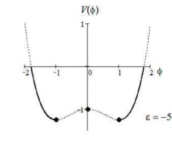
Figure 1: Mexican hat potential (dot line, $\varepsilon=-5$). In case A regular solutions terminate at the points of extremum (black points). In case B the solutions terminate on the slopes of the potential (black solid lines).

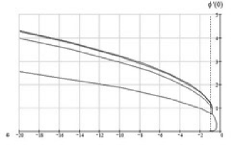
Figure 2: The area of regular configurations in the plane $\left(\varepsilon,\phi_{0}^{\prime}\right)$ for $d_{0}=4$ and $\Gamma=1.$ The upper curve is the boundary of existence of regular solutions. Other curves separate the regions with different signs of $\phi_{\infty}.$ They quickly condense to the upper curve. Below the lowest curve $\phi(l)$ does not change sign.

In case A the value of $\Gamma$ is not restricted from above. Fig 2. shows the area of regular configurations in the plane $\left(\varepsilon,\phi_{0}^{\prime}\right)$ for $d_{0}=4$ and $\Gamma=1.$ Depending on the values of $\varepsilon$ and $\phi_{0}^{\prime}$ the order parameter $\phi\left(l\right)$ tends to $+1,$ $0,$ or $-1$ as $l\rightarrow\infty.$ The sequence of curves $f_{n}\left(\varepsilon\right)$ in Fig. 2 are those where $\phi\left(l\right)\rightarrow 0$ as $l\rightarrow\infty.$ They separate the areas with different signs of $\phi_{\infty}.$ Below the first curve $f_{1}\left(\varepsilon\right)$ from the bottom, where $0<\phi_{0}^{\prime}<f_{1}\left(\varepsilon\right),$ the order parameter $\phi\left(l\right)$ doesn’t change sign. Between $f_{1}\left(\varepsilon\right)<\phi_{0}^{\prime}<f_{2}\left(\varepsilon\right)$ it changes the sign once. In the area $f_{2}\left(\varepsilon\right)<\phi_{0}^{\prime}<f_{3}\left(\varepsilon\right)$ it changes the sign twice, and so on. The curves $f_{n}\left(\varepsilon\right)$ quickly condense to the upper curve $f_{\infty}\left(\varepsilon\right)$ as $n\rightarrow\infty.$ $f_{\infty}\left(\varepsilon\right)$ is the upper boundary of existence of regular solutions (for the particular values $d_{0}=4$ and $\Gamma=1).$

The curves in Fig. 2 are those where

$$\phi_{\infty}\left(\phi_{0}^{\prime},\varepsilon,d_{0}=4,\Gamma=1\right)=0.$$ (70)

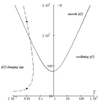
Figure 3: Case A. Map of regular solutions in the plane $(\Gamma,-\varepsilon)$ for $\phi_{0}^{\prime}=\pm\sqrt{-\frac{\varepsilon+1}{8}}$, $d_{0}=4.$ The solid curve (71) separates the regions of smooth (above) and oscillating (below) behavior of the order parameter at $l\rightarrow\infty.$ To the left of the dash curve the order parameter changes sign.

Similar curves can be shown for fixed $\phi_{0}^{\prime}$ in the plane $\left(\varepsilon,\Gamma\right).$ For instance, the dash line in Fig. 3 is the first one of the curves $\phi_{\infty}\left(\phi_{0}^{\prime}=\pm\sqrt{-\frac{\varepsilon+1}{8}},\varepsilon,d_{0}=4,\Gamma\right)=0,$ where the order parameter tends to zero at $l\rightarrow\infty$. The value $\phi_{0}^{\prime}=\pm\sqrt{-\frac{\varepsilon+1}{8}}$ $\left(\ref{Fi'0=}\right)$ corresponds to $\gamma_{0}^{\prime\prime}=0$ in $\left(\ref{relation for bound condA}\right).$ It is the case $C=0$ in (65), so that the symmetry breaking of the plain bulk is caused completely by the potential $V\left(\phi\right),$ and not by the cosmological constant. To the right of the dash line $\phi\left(l\right)$ does not change the sign.

For the potential $\left(\ref{Mexican hat}\right)$ the boundary line $\left(\ref{Boundary between mon and osc}\right)$ between oscillating and smooth $\phi\left(l\right)$ is

$$-\varepsilon_{b}=16\frac{\left(1+G\right)^{2}}{G},\quad G=\frac{d_{0}+1}{d_{0}\Gamma}.$$ (71)

It is presented in Fig. 3 (solid line). Below the solid line the order parameter $\phi\left(l\right)$ tends to its limiting value $\phi_{\infty}$ with damping oscillations (see Fig. 4), and above this curve – without oscillations, see Fig. 5.

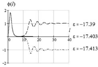
Figure 4: Oscillating solutions in the vicinity of the lower black point on the dash curve in Fig. 3.

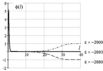
Figure 5: Smooth solutions in the vicinity of the upper black point on the dash curve in Fig. 3.

The curves in Fig. 4 correspond to the close vicinity of the lower black point on the dash curve in Fig. 3, the curves in Fig. 5– to the vicinity of the upper black point.

Case B
There are two major qualitative differences between cases A and B. In case B:

1. Parameter $\Gamma$ (69), characterizing the strength of gravitational field, is restricted from above, as it follows from (49). In the plane of parameters $(\Gamma,\varepsilon)$ the upper boundary of existence of regular solutions, found numerically, is presented in Figure 6.

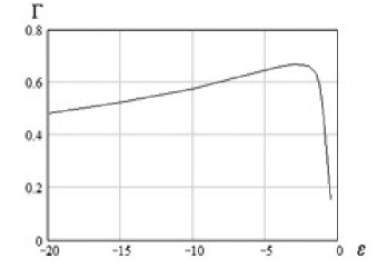
Figure 6: Case B. The upper boundary of regular solutions found numerically.

2. Regular solutions terminate with $\phi_{\infty}$ on a slope of the potential $V(\phi),$ and not at the points of extremum. See black solid parts on the dashed curve in Fig.1, where the conditions (53) and (54) are fulfilled.

The final value $\phi_{\infty}$ obeys the equation (55). In case of Mexican hat potential (67) we find

$$\phi_{\infty}^{2}=1+\frac{1}{3}\left(1+\frac{d_{0}}{\Gamma}\right)\left(\sqrt{1-\frac{3\varepsilon}{\left(1+d_{0}/\Gamma\right)^{2}}}-1\right).$$ (72)

If $\Gamma$ is small, (72) reduces to

$$\phi_{\infty}^{2}=1+\frac{\Gamma\left|\varepsilon\right|}{2d_{0}},\qquad\Gamma\ll 1,$$ (73)

and $\phi_{\infty}$ goes to a minimum of $V(\phi)$ in the limit $\Gamma\rightarrow 0$.

Typical map of regular solutions in the plane of parameters $(\phi^{\prime}_{0},\Gamma)$ is presented in Figure 7. Here $\varepsilon=-10,$ and $d_{0}=4.$

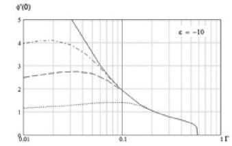
Figure 7: Map of regular solutions in the plane of parameters $(\phi^{\prime}_{0},\Gamma).$ Case B, $\varepsilon=-10,$ $d_{0}=4.$ The solid line is the upper boundary of existence of regular solutions. Dotted, dashed and dadot lines separate the regions where $\phi(l)$ changes its sign zero, once, twice, and three times. Separating lines between the regions where $\phi(l)$ changes sign more than three times are not shown.

The solid line in Figure 7 is the upper boundary of existence of regular solutions. The dotted line separates the solutions with the same sign of $\phi(l)$ (below) from the solutions with $\phi(l)$ changing sign ones (between dotted and dashed lines). Between dashed and dadot lines $\phi(l)$ changes its sign twice, and so on. There also are solutions with $\phi(l)$ changing sign more than three times, but other separating lines are not shown in the Figure 7.

The order parameter $\phi(l)$ is presented in Figure 8 for $\Gamma=0.05$, $\varepsilon=-5$, and $\phi^{\prime}(0)$ taken from the different regions in Figure 7. Solid, dotted, and dashed curves correspond to the order parameter of the same sign, changing sign once, and twice. The values of $\phi^{\prime}(0)$ are 1, 2, and 3, respectively.

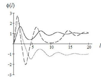
Figure 8: Case B. $\Gamma=0.05$ and $\varepsilon=-5$. Order parameter $\phi(l)$ of the same sign (solid curve), changing sign once (dotted curve), and twice (dashed curve) Corresponding values of $\phi^{\prime}(0)$ are 1, 2, and 3. In accordance with (72) $\phi_{\infty}=\pm 1.01530$.

IV.2 Neutral quantum particle in the space-time with metric (7)

A neutral spinless quantum particle is described by a scalar wave function $\chi$ with the Lagrangian

$$L_{\chi}=\frac{1}{2}g^{AB}\chi_{,B}^{\ast}\chi_{,A}-\frac{1}{2}m_{0}^{2}\chi^{\ast}\chi.$$ (74)

In the uniform bulk (while the symmetry is not broken) it is a free particle in the $D$-dimensional space-time with mass $m_{0}$ and spin zero. In the broken symmetry space-time with metric (7) it satisfies the Klein-Gordon equation

$$\frac{1}{\sqrt{-g}}\left(\sqrt{-g}g^{AB}\chi_{,A}\right)_{,B}+m_{0}^{2}\chi=0.$$ (75)

The metric (7) depends on the only one coordinate $x^{d_{0}}=l$. So the momenta, conjugate to all other coordinates, are quantum numbers. The wave function in a quantum state is

$$\chi\left(x^{A}\right)=X\left(l\right)\exp\left(-ip_{\mu}x^{\mu}+in\varphi\right),$$ (76)

where $p_{\mu}=\left(E,\mathbf{p}\right)$ is the $d_{0}$-momentum within the brane, and $n$ is the integer angular momentum conjugate to the circular extradimensional coordinate $\varphi.$ $X\left(l\right)$ satisfies the equation Bron 1

$$X^{\prime\prime}+S_{1}X^{\prime}+\left(p^{2}e^{-2\gamma}-n^{2}e^{-2\beta}-m_{0}^{2}\right)X=0.$$ (77)

The eigenvalues of $p^{2}=E^{2}-\mathbf{p}^{2}$ compose the spectrum of squared masses, as observed within the brane. Quantum number $n$ is the integer proper angular momentum of the particle. From the point of view of the observer in the brane it is the internal momentum, identical to the spin of the particle.

The equation $\left(\ref{X''}\right)$ takes the form of the Schrodinger equation

$$y_{xx}+\left[p^{2}-\textsf{V}_{g}\left(x\right)\right]y=0$$ (78)

after the substitution

$dl=e^{\gamma}dx,\qquad X\left(l\right)=y\left(x\right)/\sqrt{f\left(x\right)},$   $f\left(x\right)=\exp\left\{-\frac{1}{2}\left[\left(d_{0}-1\right)\gamma+\beta\right]\right\}.$

The gravitational potential

$$\textsf{V}_{g}\left(x\right)=e^{2\gamma}\left(e^{-2\beta}n^{2}+m_{0}^{2}\right)+\frac{1}{2}\frac{1}{\sqrt{f}}\frac{d}{dx}\left(\frac{1}{f^{1/2}}\frac{df}{dx}\right)$$ (79)

determines the trapping properties of particles to the brane. The trapping is insured by the exponentially growing warp factor $e^{2\gamma}$: in view of (52) and (56) in both cases A and B $\gamma_{\infty}^{\prime}$ are positive constants. In terms of $U$, $S_{1},$ and $\phi$ (42) the dependence of the gravitational potential (79) on the distance $l$ is

$$\textsf{V}\left(l\right)=e^{2\gamma}\left(e^{-2\beta}n^{2}+m_{0}^{2}\right)+\frac{e^{2\gamma}}{4}\frac{\left(d_{0}S_{1}-U\right)\left(U+\left(d_{0}+2\right)S_{1}\right)}{\left(d_{0}+1\right)^{2}}+\frac{e^{2\gamma}}{2}\left(\kappa^{2}\frac{\partial V}{\partial\phi}\phi+\frac{U\left(S_{1}-d_{0}U\right)}{d_{0}+1}\right).$$ (80)

IV.3 Oscillations

The oscillations of the order parameter $\phi(l)$ give rise to the oscillations of the gravitational potential (79), see Figures 9,10.

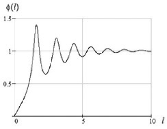
Figure 9: Case A. A solution with oscillating order parameter $\phi(l).$ Here $d_{0}=4,$ $\varepsilon=-2,$ $\Gamma=10,$ $\phi^{\prime}(0)=\sqrt{-\frac{\varepsilon+1}{8}}$.

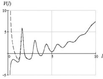
Figure 10: Case A. Gravitational potential $\textsf{V}_{g}\left(l\right)$ (80) for the same set of the parameters as in Fig.8, $d_{0}=4,\varepsilon=-2,\Gamma=10,\phi_{0}^{\prime}=\sqrt{-\frac{\varepsilon+1}{8}}$. The initial mass of a test particle is set $m_{0}=0$. The solid curve corresponds to the angular momentum $n=0$, and the dashed one – to $n=1$.

In terms of $\left(\ref{G=}\right)$ the eigenvalues $\left(\ref{eigenvaluesA}\right)$ are

$$\lambda_{\pm}=-\sqrt{-\frac{\varepsilon}{8\left(G+1\right)}}\left[1\pm\sqrt{1+\frac{16}{\varepsilon G}\left(G+1\right)^{2}}\right].$$ (81)

The less is $\left|\varepsilon\right|$ the more oscillations display themselves. In the limiting cases of small and large $\Gamma$ the frequencies of oscillations

$$\left|\textrm{Im}\lambda\right|=\left\{\begin{array}[]{c}\sqrt{2},\quad\Gamma\rightarrow 0,\\ \sqrt{2\left(1+\frac{1}{d_{0}}\right)\Gamma},\quad\Gamma\rightarrow\infty\end{array}\right.$$

do not depend on $\varepsilon$ as $l\rightarrow\infty.$ At $\left|\varepsilon\right|\sim 1$ and $\Gamma\gg 1$ the gravitational potential has many points of minimum, see Fig. 10.

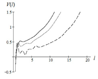
Figure 11: Case B. Gravitational potential $\textsf{V}_{g}\left(l\right)$ (80) for the same sets of the parameters as for the curves of order parameter in Fig.8. $d_{0}=4$, $\varepsilon=-5,$ $\Gamma=0.05,$ $\phi^{\prime}(0)=1$ (solid curve), $2$ (dotted curve), and $3$ (dashed curve). The initial mass of a test particle $m_{0}=0$ and the angular momentum $n=0$.

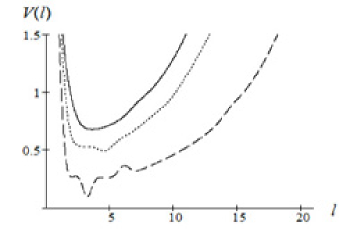
Figure 12: Case B. Gravitational potential $\textsf{V}_{g}\left(l\right)$ (80) for a particle with mass $m_{0}=0$ and angular momentum $n=1$. The sets of the parameters are the same as in Fig.11: $d_{0}=4$, $\varepsilon=-5,$ $\Gamma=0.05,$ $\phi^{\prime}(0)=1$ (solid curve), $2$ (dotted curve), and $3$ (dashed curve). The difference between angular momenta $n=0$ and $n=1$ is essential only near the center.

The length scale $a$ (68) remains an arbitrary parameter of the theory. The physical interpretation is different in the limiting cases of large and small $a.$ If $a$ is extremely large, each minimum of the potential $V(l)$ (80) forms its own brane. If the potential barrier is high, the branes are separated from one another.

In the opposite limit, when the scale length $a$ is extremely small, all points of minimum are located within one common brane, and in the spirit of Kalutza-Kline the points of minimum are beyond the resolution of modern devices.

Low energy particles can be trapped by the points of minimum of the potential (79). Identical in the bulk neutral spin-less particles, being trapped in the different minimum points, acquire different masses and angular momenta. If the scale length $a$ is extremely small, then they appear to the observer in brane as different particles with integer spins.

V Concluding remarks

As a result of rather wearing derivations of the energy-momentum tensors we get more simple equations than in the case of scalar multiplet models.

The main features of spontaneous symmetry braking with a hedge-hog type vector order parameter in comparison with the widely used previously scalar multiplet model are presented in table 1.

Table 1: Mutual comparison of main features of regular solutions employing the vector order parameter (cases A and B) with the scalar multiplet model. $n_{V}$ is the number of free parameters of the symmetry breaking potential $V(\phi)$.

$\begin{pmatrix}\textbf{Property}&\textbf{Case A}&\textbf{Case B}&\textbf{Scalar multiplet}\\ $Order of Einstein equations$&3&3&4\\ $Number of free parameters$&n_{V}+1&n_{V}+1&n_{V}\\ $Fine tuning$&${no need}$&${no need} $&\textit{in some cases}\\ r(\infty)&\infty&\infty&\infty,r_{m},0\\ $Matter trapping$&yes&yes&yes\\ $Presence of $dV/d\phi$ in equations $&yes&no&no\\ $Presence of $V$ in equations$&no&yes&yes\\ $Derivation of $T_{IK}&wearing&wearing&easy\\ $Equations are$&${most simple}$&\textit{more simple}&\textit{simple}\\ $Strength of gravitational field $\Gamma&${arbitrary}$&\textit{restricted from above}&\textit{arbitrary}\\ \end{pmatrix}$

The solutions have additional parametric freedom: in both cases A and B the inclination $\phi_{0}^{\prime}$ is arbitrary within a whole interval of values (see Figures 2 and 6), and not only at some fixed values as in the scalar multiplet case. It means that the possibility of existence of the brane world is not connected with any restrictions of fine-tuning type. The origin of the additional parametric freedom is the order of equations, which in case of vector order parameter is less than in scalar multiplet models.

All regular configurations display trapping properties. Oscillating behavior of the order parameter, especially in case A, gives rise to existence of several points of minimum of the attractive potential (80) at different energy levels. Particles, trapped at different points of minimum, acquire different masses. If we assume that the length scale $a$ (68) is extremely small, it can be a reason of the observed hierarchy of masses. Angular momentum of extra-dimensional motion $n$ is also a quantum number. It appears to the observer on brane as an internal momentum of the particle which can be scarcely separated from its spin.

Most elementary particles have half-integer spins. The simple case of spontaneous symmetry breaking, considered above, can not connect the origin of half-integer spins with extra-dimensional angular momenta. Half-integer spins in General Relativity is still a problem.

References

- (1) K.A.Bronnikov and B.E.Meierovich. Zh.Eksp. Teor. Fiz. Vol. 133, No. 2, pp. 293-312 (2008).
- (2) L.D.Landau and E.M.Lifshits. Field Theory. “Nauka”, Moscow, 1973.
- (3) J.M.Cline, J.Descheneau, M.Giovannini, and J.Vinet. E-print archives, hep-th/0304147v2.