Self-consistent theory of capillary-gravity-wave generation by small moving objects

Abstract

We investigate theoretically the onset of capillary-gravity waves created by a small object moving at the water-air interface. It is well established that, for straight uniform motion, no steady waves appear at velocities below the minimum phase velocity $c_{\text{min}}=23\,{\rm cm/s}$. At higher velocities the emission of capillary-gravity waves creates an additional drag force. The behavior of this force near the critical velocity is still poorly understood. A linear response theory where the object is replaced by an effective pressure source predicts a singular behavior for the wave drag. However, experimental data tends to indicate a more continuous transition. In this article, we show that a proper treatment of the flow equations around the obstacle can regularize wave emission, even in the linear wave approximation, thereby ensuring a continuous behavior of the drag force.

I Introduction

An object moving uniformly in an incompressible liquid experiences a drag force that can have several physical origins: viscous drag, hydrodynamic interaction with close-by boundaries, or the force due to the emission of waves. The waves, on which we focus in the present paper, appear when the object moves in the vicinity of a deformable surface such as an air–liquid interface (LanLif59, ). They carry away momentum from the object which is sensed as the wave drag of the moving object. The type of waves we expect on an air-liquid interface are capillary gravity waves (LanLif59, ; Acheson, ). Their dispersion relation in an unbounded inviscid liquid of infinite depth is well known to be $\omega^{2}=gk+\gamma k^{3}/\rho$. It relates the oscillation frequency $\omega$ to the wave number $k$ and depends on the gravity constant $g$, fluid density $\rho$ and on the surface tension $\gamma$. The wave velocity $c(k)=\omega/k$ is readily obtained as $c(k)=(g/k+\gamma k/\rho)^{1/2}$. The dispersive nature of capillary-gravity waves creates a complicated wave pattern around a moving object, yielding a finite wave drag. In naval design the wave drag is an important source of resistance, which stimulated the development of approximate theoretical methods (Lighthill, ; Lamb, 1993; Rayleigh, ; Kelvin, ; Milgram, ; Burghelea1, ). These methods are valid only for objects larger than the capillary length $\kappa^{-1}=\sqrt{\gamma/(\rho g)}$ (RapGen96, ). The case of objects of extension comparable to $\kappa^{-1}$ has been overlooked for a long time in the literature, but has attracted strong interest in the context of insect locomotion on water surfaces (Tucker, ; Denis, ; Bush, ; Nachtigall1965, ). In particular, some insect species (for example wiggling beetles) may take advantage of the generation of capillary-gravity waves for echo-location purposes Denis2 ; Bendele . In particular, recent observation of the behavior of Gyrinidae suggest that they select their swimming speed by minimizing the sum of wave and viscous drags (VoiCas09, ; Alexander, ; Buhler, ).

The first theoretical calculation in this regime predicted a discontinuity of the wave drag $R_{w}$ at a critical velocity given by the minimum of the wave velocity $c_{\text{min}}=(4g\gamma/\rho)^{1/4}$ for capillary gravity waves (RapGen96, ). For water this evaluates to $c_{\text{min}}\approx 23\,\textrm{cm/s}$. An object moving at constant velocity $V<c_{\text{min}}$ does not generate steady waves, and the wave resistance vanishes. Emission of steady waves becomes possible only when $V>c_{\text{min}}$, leading to the onset of a finite wave drag. This striking behavior is similar to the well-known Cherenkov radiation emitted by charged particles (Cherenkov, ), to the onset of wave drag for supersonic aircrafts (supersonic, ) or to the Zeldovich–Starobinsky effect in general relativity (Zeldovich, ). The minimum in the dispersion relation, responsible for this behavior, renders the problem challenging. Two experiments addressed the problem of the behavior of wave resistance at a liquid–air interface. While the disappearance of wave drag was confirmed for $V<c_{\text{min}}$, opposite conclusions were reached concerning the existence of a discontinuity at the critical velocity $V=c_{\text{min}}$. In a first experiment by Browaeys et al. (2001) the bending of a narrow fiber in contact with the liquid surface was used to probe the wave drag. The results evidenced the presence of a jump at $V=c_{\text{min}}$. However, during these measurements the contact line between the fluid and the fiber was free to move, thus creating an uncontrolled contribution to the measured force. A second experiment was made by Burghelea & Steinberg (2002) in which an ingenious feedback system fixed the immersion depth of the object. This experiment concluded on a continuous increase of wave drag around $V=c_{\text{min}}$.

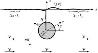
Figure 1: Geometry of the submerged cylinder and of the free surface above. The far-field velocity is indicated by the arrows $\mathbf{V}$.

While it was shown recently (CheCheRap08, ) that the threshold $V=c_{\text{min}}$ exists only for an object moving at constant velocity without acceleration, a theoretical understanding of the scaling of wave resistance is still missing. The theoretical descriptions which are available replace the moving object by an external pressure source applied at the air-liquid interface. The hydrodynamic problem is then reduced to a linear response theory in the pressure field which has singularities around $V=c_{\text{min}}$ if viscosity is neglected (RapGen96, ; Richard, ; CheRap03, ). A self-consistent determination of the pressure distribution was attempted in Ref. (CheRap03, ). While this theory succeeded in removing the singularity at $V=c_{\text{min}}$, it leads to the somewhat unrealistic prediction that the applied pressure field vanishes at $V=c_{\text{min}}$. An alternative approach by Sun & Keller (2001) is based on an asymptotic matching technique and works for velocities much larger than $c_{\text{min}}$. In order to develop a theory of wave drag valid for $V\simeq c_{\text{min}}$, we note that the linear response theory is successful at reproducing the wave pattern created in the experiments even for velocities very close to $c_{\text{min}}$. This suggests that it is possible to understand the behavior of $R_{w}$ in a theory where linear capillary-gravity waves are coupled to an accurate hydrodynamic description of the flow around the moving object. This theory is developed in the present paper.

In the situation we have in mind, the perturbation of the free surface does not come from an external pressure distribution as it was the case in Ref. (RapGen96, ). Also, we avoid the difficulties arising from an immersed perturbing needle of Ref. (CheRap03, ). Instead, we here use a completely submerged object, which is, for reasons of a dimensionality reduction, a cylinder. It has radius $R$ and is at depth $H$ below the free surface, as is depicted in Fig. 1. Notice that the dimension has implications on the nature of the transition near $c_{\text{min}}$ which we want to describe and might limit comparisons with experimental data.

The liquid flows only perpendicularly to the axis of the cylinder, and we require only $x$ and $z$ coordinates. This system has been analyzed by Lamb (1993) without taking into account the mutual interaction between the two perturbations, namely the one created by the moving object and the one by the emitted waves. He limited his discussion to particles larger than the capillary length $\kappa^{-1}$ by neglecting the capillary contribution in the dispersion. We here regard the other case of small objects, where it becomes necessary to treat the mutual interaction between the two perturbations correctly.

Generally speaking, the larger the ratio $H/R$, the better work the two theories presented below in Secs. II and V. The numerical example in Sec. IV for $H/R=5/3$, however, shows that the theories are valid already for cylinders quite close to the surface. This observation is the reason why we are convinced that the completely submerged cylinder presents a useful approach to understand the experimental setup in which a partially immersed object was used.

II Flow equations

We describe the velocity field in the reference frame of the cylinder. The far-field velocity is thus a non-zero uniform velocity $\mathbf{V}$. The velocity field is assumed to be irrotational, given by a velocity potential, where we immediately isolate the far-field velocity and use only the potential $\phi(x,z)$ of the perturbations due to the obstacle and to the waves,

$$\mathbf{v}(x,z)=\mathbf{V}+\boldsymbol{\nabla}\phi(x,z).$$ (1)

The incompressibility condition for the fluid reads

$$\Delta\phi=0.$$ (2)

This equation is complemented by boundary conditions at the air-liquid interface and at the surface of the cylinder. The kinematic boundary condition reads

$$\mathbf{n}\mathbin{\boldsymbol{\cdot}}(\mathbf{V}+\boldsymbol{\nabla}\phi)=0,$$ (3)

with the normal vector $\mathbf{n}$ oriented as in Fig. 1. For the deformable air–liquid interface the boundary condition is

$$\rho V^{2}\partial_{x}^{2}\phi+\rho g\partial_{z}\phi-\gamma\partial_{x}^{2}\partial_{z}\phi=0\;\;(\text{at}\quad z=0).$$ (4)

This boundary condition is obtained as follows. Using a height profile $\zeta(x)$, the kinematic boundary condition becomes for a nearly flat interface ($\partial_{x}\zeta\ll 1$),

$$\partial_{z}\phi-\partial_{x}\zeta(V+\partial_{x}\phi)=0.$$ (5)

Additionally, we have Laplace’s law and Bernoulli’s equation,

$$-p(x,\zeta(x))+p^{\text{air}}=\gamma\partial_{x}^{2}\zeta,$$ (6)

$$\frac{\rho}{2}\mathbf{v}^{2}(x,\zeta(x))+\rho g\zeta(x)+p(x,\zeta(x))=\textit{const},$$ (7)

with $\gamma$ the surface tension and with $p^{\text{air}}$ the pressure above the interface, which is assumed to be a constant. The curvature of the interface has been linearized. The boundary condition (4) is obtained by inserting Laplace’s law into the Bernoulli’s equation, linearized in $\phi$. A derivative with respect to $x$ and multiplying with $\partial_{x}\phi$ allows to eliminate the height profile $\zeta$, using Eq. (5). Terms which are either quadratic in $\phi$ or bilinear in $\phi$ and $\zeta$ are neglected as second-order perturbations.

Figure 2: Overview of the variable transformations of the full theory in Secs. II and III (upper panel), and of the dipolar model in Sec. V (lower panel).

The problem we will solve in the following consists of the Laplace equation (2) for the unknown $\phi(x,z)$, together with the two boundary conditions (3) and (4). The flow disturbance must further vanish at very large depths: $\partial_{z}\phi\rightarrow 0$ when $z\rightarrow-\infty$. These equations can not be solved directly by numerical means in real space, such as by a finite element method, since the waves emitted by the cylinder propagate to infinity whereas any discretization is done in a finite domain. Hence, additional analytic transformations are needed to cast the problem in a more accessible form. An overview of the following transformations is provided in Fig. 2. We split the potential into two components with different physical origins $\phi=\phi_{0}+\phi_{1}$. The term $\phi_{0}$ is dominated by the perturbation stemming from the sphere, and $\phi_{1}$ is mainly the perturbation from the free surface. Of course, both perturbations have to mutually respect the presence of the other boundary. In more precise terms, the potential $\phi_{0}$ obeys the Laplace equation with the boundary condition $\mathbf{n}\mathbin{\boldsymbol{\cdot}}\boldsymbol{\nabla}\phi_{0}=-V_{C}(\theta)$ at the surface of the cylinder and $\nabla\phi_{0}\rightarrow 0$ for $r\rightarrow\infty$.

The unknown function $V_{C}(\theta)=\mathbf{n}\mathbin{\boldsymbol{\cdot}}(\mathbf{V}+\nabla\phi_{1})$ describes the flow created by $\mathbf{V}$ and the wake at the cylinder surface (hence Eq. (3) is always verified). The flow $\boldsymbol{\nabla}\phi_{1}$ created by the surface-waves is oscillatory in the $x$ direction and decays exponentially with the depth $z$. These properties are naturally captured by the integral representation commonly used in theories of surface waves (Lighthill, ; RapGen96, ),

$$\phi_{1}(x,z)=\frac{1}{2\pi}\int dke^{ikx}e^{|k|z}A(k),$$ (8)

where $k$ denotes the wave number. The two unknown potentials $\phi_{0}(x,z)$ and $\phi_{1}(x,z)$ are now replaced by the two unknown functions $V_{C}(\theta)$ and $A(k)$. Those have to be determined self-consistently in order to satisfy the boundary conditions Eqs. (3) and (4). This procedure requires an expression of $\phi_{0}$ in terms of $V_{C}$, which is given by the integral representation

$$\phi_{0}(r,\theta)=-\frac{R}{\pi}\int\log|re^{i\theta}-Re^{i\theta^{\prime}}|V_{C}(\theta^{\prime})d\theta^{\prime}$$ (9)

which uses the polar coordinates depicted in Fig. 1. Notice that the origin of these polar coordinates coincides with the cylinder axis while the origin of the Cartesian coordinates $x,z$ is located at the free interface above the obstacle. Relation (9) is either obtained by expanding $V_{C}(\theta)$ as a Fourier series and by solving the Laplace equation for each term. An alternative way is to use the full Green function of the Neumann problem in the circle (Jackson75, ; Schindler06, ). The logarithmic integral kernel appears as a consequence the fundamental solution of the Laplace equation in two dimensions. Notice that the part of the Green function which enforces the Neumann boundary condition is also logarithmic.

The boundary condition (4) leads to a first relation between $V_{C}(\theta)$ and $A(k)$. Since it is invariant under translations in the $x$ direction, it takes a simple form in Fourier space,

$$A(k) =-\frac{1}{|k|}\>\frac{\omega^{2}(k)+V^{2}k^{2}}{\omega^{2}(k)-V^{2}k^{2}}V_{z}(k)\quad\text{with}$$ (10)

$$V_{z}(k) :=\int dxe^{-ikx}\partial_{z}\phi_{0}(x,0)$$ (11)

The expression of $V_{z}(k)$ as a function of $V_{C}(\theta)$ is readily obtained by inserting Eq. (9) into the above Eq. (11). The integral with respect to $x$ can be evaluated analytically, which yields

$$V_{z}(k)=-R\int e^{-|k|(H-R\sin(\theta^{\prime})}e^{-ikR\cos(\theta^{\prime})}V_{C}(\theta^{\prime})\>d\theta^{\prime}$$ (12)

The exponential factors arise from the Fourier transform of the derivatives of the logarithmic kernel in Eq. (9). We have now expressed the unknown function $A(k)$ in terms of the other, $V_{C}(\theta)$. The remaining kinematic boundary condition (3) at the cylinder surface now serves as a closed equation for determining $V_{C}(\theta)$,

$$V_{C}(\theta)=\mathbf{n}\mathbin{\boldsymbol{\cdot}}(\mathbf{V}+\boldsymbol{\nabla}\phi_{1})$$ (13)

$$=\mathbf{n}\mathbin{\boldsymbol{\cdot}}\Bigl{(}\mathbf{V}-\frac{\boldsymbol{\nabla}}{2\pi}\int dk\>\frac{e^{ikx}e^{|k|z}}{|k|}\>\frac{\omega^{2}(k){+}V^{2}k^{2}}{\omega^{2}(k){-}V^{2}k^{2}}V_{z}(k)\Bigr{)}$$ (14)

By injecting $V_{z}$ from Eq. (12) into the last integral and by changing the order of integration, $V_{C}(\theta)$ is found to satisfy an integral equation of Fredholm’s second kind

$$V_{C}(\theta)=V\cos\theta+\frac{1}{2\pi}\int K(\theta,\theta^{\prime})V_{C}(\theta^{\prime})d\theta^{\prime},$$ (15)

with the kernel function

$$K(\theta,\theta^{\prime})=R\int\bigl{[}i\;{\rm sgn}(k)\cos\theta+\sin\theta\bigr{]}\frac{\omega^{2}(k)+V^{2}k^{2}}{\omega^{2}(k)-V^{2}k^{2}}\\ {}\times e^{ikR(\cos\theta-\cos\theta^{\prime})}e^{-|k|(2H-R\sin\theta-R\sin\theta^{\prime})}\>dk$$ (16)

In this integral, singular pole contributions appear when the denominator vanishes, $\omega^{2}(k)-V^{2}k^{2}=0$. This happens only for $V>c_{\text{min}}$. The two positive solutions of this equation, which we call $k_{g}$ and $k_{c}$ ($k_{c}>k_{g}$) correspond to gravity waves and capillary waves, respectively. In the far-field regimes, they dominate the flow and thus correspond to the inverse wavelengths found before and behind the obstacle. Directly above the cylinder no unique wavelength can be identified. In order to ensure that waves only leave the object and are not coming back from infinity, we introduce an infinitesimal imaginary part into the dispersion relation. This term can be understood as an infinitesimal viscous term (RapGen96, ; CheRap03, ). With the correct choice of its sign, the denominator becomes $\omega^{2}(k)-V^{2}k^{2}-i\varepsilon k$. Notice that this choice also ensures that capillary waves are emitted to the front and that gravity waves rest at the rear of the obstacle.

III Wave drag

Provided that the self-consistent Eq. (15) has been solved to find the function $V_{C}$, one can reconstruct the flow everywhere in the domain around the obstacle. This procedure requires to calculate in turn $\phi_{0}$, $A(k)$, and $\phi_{1}$, using Eqs. (9), (10), and (8). Once the flow is known, two different strategies offer themselves for the calculation of the wave drag. Both are indicated in the upper part of Fig. 2. The first, which is conceptually simpler, passes over the pressure field $p(x,z)$, using Bernoulli’s equation

$$\frac{\rho\mathbf{v}^{2}(x,z)}{2}+\rho gz+p(x,z)=\frac{\rho V^{2}}{2}.$$ (17)

The pressure field can then be integrated around the surface of the cylinder to find the total drag force. In an inviscid fluid, d’Alembert’s theorem ensures that the drag caused by the emitted surface waves is the only contribution to the drag force (LanLif59, , § 11). The wave drag then reads:

$$R_{w}=-\frac{1}{V}\mathbf{V}\mathbin{\boldsymbol{\cdot}}\oint_{S_{R}}dA(x,z)\,p(x,z)\,\mathbf{n}.$$ (18)

The second approach to calculate the wave drag makes use of the power carried away by the waves. For the linear waves used here, the relation between this power and the amplitude of the velocity oscillations in the far-field regime are well known (RapGen96, ). The oscillations in the far-field regime are of the form $\zeta(x)=a\cos(kx+h)$. The amplitudes $a_{c},a_{g}$, the wave numbers $k_{c},k_{g}$ and the phases $h_{c},h_{g}$ are different for capillary and for gravity waves. Each energy density of the particular wave depends quadratically on the amplitude,

$$E(k)=\frac{1}{2}\rho c(k)^{2}\,ka^{2}.$$ (19)

This energy density may alternatively be expressed in terms of the amplitude of the velocities, denoted by $v_{z,\infty}$, which is related to the amplitude $a$ of the deformation by $v_{z,\infty}=Vka$. This relation is a consequence of the linearized kinematic boundary condition (5). It allows to determine the amplitude $a$ from the flow, once the function $V_{C}(\theta)$ is known. The two energy densities allow to calculate the power carried away by the waves, from which the drag results as (RapGen96, ),

$$R_{w}=\frac{V-\omega^{\prime}(k_{c})}{V}E(k_{c})-\frac{V-\omega^{\prime}(k_{g})}{V}E(k_{g}).$$ (20)

The energy of each wave is transported at the group velocity $\omega^{\prime}$.

The two expressions (18) and (20) for the wave drag are equivalent. Their comparison allows to verify the accuracy of the numerical solutions below.

IV Numerical results

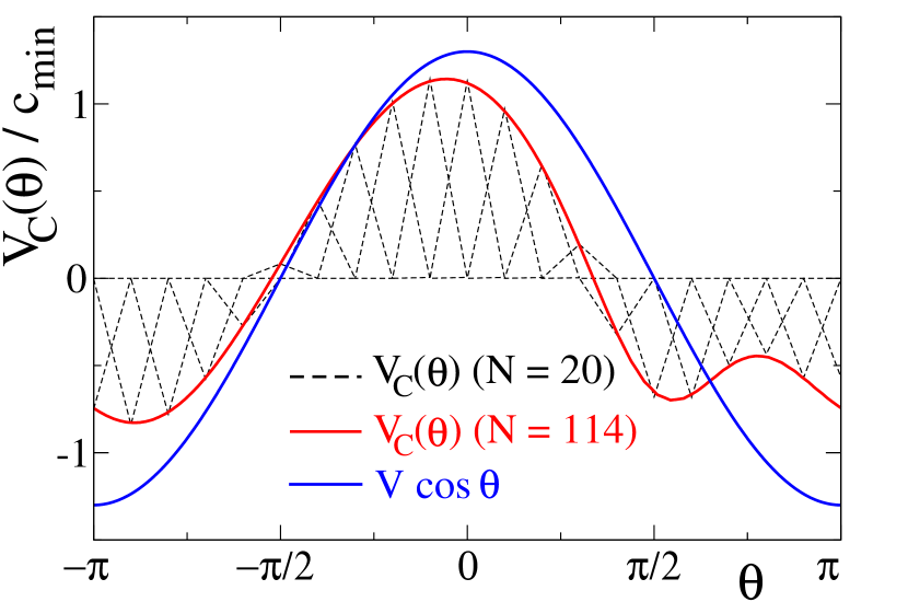
Figure 3: (Color online) Numerical solution of Eq. (15). The dashed lines represent the discretisation with linear finite elements. Parameters: $H\kappa=0.5$, $R\kappa=0.3$, and $V=1.3c_{\text{min}}$.

The self consistent equation Eq. (15) can be solved by numerical methods. Our first step is to create a numerical table of the values of the kernel $K(\theta,\theta^{\prime})$, the integral in the definition of the kernel is computed using standard numerical routines from the GSL library (gsl, ). It provides special discretizations for calculating principal values which appear in Eq. (16) due to the singular integrand. The equation Eq. (15) is then discretized using finite elements. The function $V_{C}(\theta)$ is approximated using a finite set of $N$ basis functions $\phi_{n}(\theta)$.

$$V_{C}(\theta)=\sum_{n=1}^{N}c_{n}\phi_{n}(\theta)$$ (21)

For simplicity we have chosen a basis of $N$ piecewise linear hat functions with periodic boundary conditions on the $(-\pi,\pi)$ interval. Fig. 3 shows an example of such an approximation for a small number of elements $N=20$. This expression for $V_{C}(\theta)$ is then inserted in Eq. (15) and Galerkin’s method is used to convert it into a matrix equation of size $N\times N$. Namely we multiply Eq. (15) by one of the function $\phi_{m}(\theta)$ and integrate over the angle $\theta$. This leads to a linear equation on the coefficients $c_{n}$:

$$\sum_{n}[(\phi_{m},\phi_{n})-\frac{1}{2\pi}(\phi_{m},K\phi_{n})]c_{n}=V(\phi_{m},\cos\theta)$$ (22)

where we have introduced the notation $K\phi_{n}(\theta)=\int K(\theta,\theta^{\prime})\phi_{n}(\theta^{\prime})d\theta^{\prime}$ and defined scalar product between two arbitrary functions $f(\theta)$ and $g(\theta)$ as

$$(f,g):=\int f(\theta)g(\theta)d\theta$$ (23)

In a last step the system Eq. (22) is solved using a LU decomposition (numres, ). The integrals involved in the calculation of the scalar products are determined numerically (gsl, ). It is possible to check the convergence of our numerical procedure by inserting the obtained approximation for $V_{C}(\theta)$ into Eq. (15). The degree of accuracy can then be estimated from the difference between the left and right hand side of Eq. (15). For the typical number of elements we use in our simulations $N\simeq 110$ the relative difference is of the order of $10^{-3}$.

Figure 3 presents the solution of Eq. (15) for the geometrical parameters $H\kappa=0.5$, $R\kappa=0.3$ and a flow velocity of $V=1.3c_{\text{min}}$. It is compared with the source term of the integral equation $V\cos\theta$ which results if the contribution from the surface waves is neglected. As can be seen, the function $V_{C}(\theta)$ is strongly modified by the self-consistent interaction between the cylinder and the emitted capillary-gravity waves.

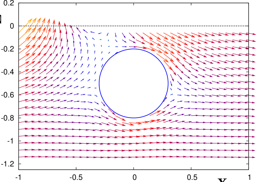
Figure 4: (Color online) Visualization of the flow velocity around the cylinder. The velocities are represented by arrows the size of which is proportional to the velocity magnitude. The color code is yellow/gray for large magnitudes and blue/black of small ones. Parameters as in Fig. 3.

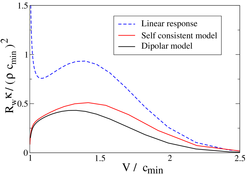
Figure 5: (Color online) Wave drag as a function of the far-field velocity $V$ for the parameters for $H\kappa=0.5$ and $R\kappa=0.3$. The results of three different models are presented: the dashed curve corresponds to a linear response calculation where $V_{C}=V\cos\theta$, the red (gray) curve corresponds to a self-consistent calculation using Eq. (15) and the black curve corresponds to the dipolar model explained in section IV.

Once the function $V_{C}(\theta)$ has been determined we can calculate the flow in all the space $z<0$ around the cylinder following the steps described in section II. The velocity field around the cylinder for the parameters of Fig. 3 is depicted in Fig. 4. Notice that the flow obeys the kinetic boundary condition on the sphere given by Eq. (3) which confirms our numerical procedure.

Using the results from Sec. III, we can now calculate the wave drag as a function of the externally applied flow velocity $V$. Figure 5 shows this function, as determined numerically from both, the direct integration of the pressure field around the sphere (18), and from the energy balance in Eq. (20). Their difference in Fig. 5 is smaller than the line width. At velocities $V$ close to the critical value $c_{\text{min}}$, the drag vanishes continuously. This behavior is qualitatively different from that found from linear response theory with an external pressure field as perturbation, as it predicts a divergence at $c_{\text{min}}$  (RapGen96, ). Our approach reduces to this linear response theory if, instead of solving the self consistent Eq. (15), $V_{C}(\theta)$ is set to the result $V\cos\theta$ for a cylinder moving in a quiescent inviscid liquid without surface. The wave drag obtained in this case diverges close to $V=c_{\text{min}}$ as shown by the dashed curve on Fig. 5. At large velocities, the wave drag determined from the self consistent model curve rejoins the curve from linear response.

The observation in Fig. 5, that the drag is a continuous function at the critical velocity, constitutes the central result of the present work. The regularization is achieved by the self-consistent treatment of the emitted waves, which takes into account the mutual interaction between the perturbations created by the cylinder and the waves, respectively. The physical origin of the regularization can be understood with a simpler model which does not require the full solution of the self-consistent equation. This model will be detailed in the following section, where we derive a square-root scaling for the wave drag close to $c_{\text{min}}$.

V Dipolar model

We now treat the interaction between the wake and the cylinder in an approximate manner. Instead of enforcing the exact kinematic boundary condition (3) at all points on the cylinder, we impose it only as an averaged constraint. This approach assumes that the flow $\mathbf{v}_{1}=\boldsymbol{\nabla}\phi_{1}$, created by the waves, is homogeneous around the cylinder. The response of the cylinder is now reduced to a simple dipolar potential which describes the response to a yet unknown uniform flow $(\mathbf{V}+\mathbf{v}_{1})$,

$$\phi_{0}=R^{2}(\mathbf{V}+\mathbf{v}_{1})\mathbin{\boldsymbol{\cdot}}\boldsymbol{\nabla}\log r.$$ (24)

The name “dipolar” arises from the analogy with the potential of a dipole in two-dimensional electrostatics. This approximation reduces the complexity of the equation (9). Figure 2 summarizes the necessary transformations in the same way as it was done for the sections above. Instead of determining a whole function $\phi_{0}$ we must now only find two parameters $v_{1,x}$ and $v_{1,z}$. With these parameters, the function $V_{C}(\theta)$ from Sec. II assumes the form $V_{C}(\theta)=(V+v_{1,x})\cos\theta+v_{1,z}\sin\theta$, which can be used immediately to calculate the unknown function $A(k)$. The self-consistent equation (15) for $V_{C}$ is thus replaced by a linear set of two equation for the parameters. The solution is

$$\left(\begin{array}[]{c}V+v_{1,x}\\ v_{1,z}\end{array}\right)=\frac{V}{(1-I_{1})^{2}+I_{2}^{2}}\left(\begin{array}[]{c}1-I_{1}\\ -I_{2}\end{array}\right),$$ (25)

with the shortcuts

$$I_{1} =\int\frac{dk}{2\pi}\pi R^{2}e^{-2H|k|}|k|\frac{\omega^{2}(k)+V^{2}k^{2}}{\omega^{2}(k)-V^{2}k^{2}},$$ (26)

$$I_{2} =\int\frac{dk}{2\pi}\pi R^{2}e^{-2H|k|}ik\frac{\omega^{2}(k)+V^{2}k^{2}}{\omega^{2}(k)-V^{2}k^{2}}.$$ (27)

In order to obtain the wave drag $R_{w}$ from this result, we follow the same steps as in Sec. III. This time, we can do them analytically, not only numerically, thanks to the simple form of the potential $\phi_{0}$. In this treatment, we prefer the energy balance argument instead of the pressure integral. In the far-field, $x\to\pm\infty$, we find the wave amplitude as follows,

$$a=2\pi R^{2}\frac{kVe^{-H|k|}}{|\omega^{\prime}(k)-V|}\frac{1}{\sqrt{(1-I_{1})^{2}+I_{2}^{2}}}\;,\;c(k)=V$$ (28)

In the course of this calculation, we pass from $\phi_{0}$ to $A(k)$, using Eqs. (10) and (11). In the far field regime the only contribution to the flow arises from the waves. The flow potential $\phi_{1}$ created by the waves is given by a Fourier-Laplace transform of $A(k)$ (see Eq. (8)). In the asymptotic regime $|x|\rightarrow\infty$ we can keep only the contributions from the emitted waves of fixed wave numbers $k=k_{c},k_{g}$. They appear from the delta function contribution of the integration around the poles of $A(k)$, using the identity (MatWal70, , p. 481):

$$\lim_{\varepsilon\to 0}\frac{1}{\omega^{2}(k)-V^{2}k^{2}-i\varepsilon k}$$

$$=\textrm{P.v.}\frac{1}{\omega^{2}(k)-V^{2}k^{2}}+i\pi\textrm{sgn}(k)\,\delta\bigl{(}\omega^{2}(k)-V^{2}k^{2}\bigr{)},$$ (29)

where P.v. denotes the Cauchy principal value and the delta function can be transformed as:

$$\delta\bigl{(}\omega^{2}(k)-V^{2}k^{2}\bigr{)}=\sum_{k_{i}:c(k_{i})=V}\frac{\delta(k{-}k_{i})}{2V|k_{i}|\>|\omega^{\prime}(k_{i})-V|}.$$ (30)

Now, that we have an expression for the deformation amplitude $a$, we can find the wave drag using Eqs. (19) and (20). The auxiliary integrals $I_{1}$ and $I_{2}$ are calculated numerically. The result are displayed in Fig. 5 and show that the dipolar model reproduces the behavior of the exact solution from Sec. II. The accuracy of the dipolar model can be understood because the radius of the cylinder is small compared to the capillary wave length $R=0.3\kappa^{-1}$. Hence the flow is reasonably uniform on this scale. A good agreement is found when $V\to c_{\text{min}}$ because the emitted wavelengths tend both to the same value $\kappa^{-1}$, which is larger than the object size. At higher velocities, where the emitted wavelengths differ, the agreement decreases because the shorter one may become smaller than the object size.

Our aim now is to find the square-root behavior of the drag force, $R_{w}\propto\sqrt{V-c_{\text{min}}}$ in the frame of the dipolar model. In order to do so, we analyze the scaling of the wave amplitude in Eq. (28) in the vicinity of $c_{\text{min}}$. We then use Eqs. (19) and (20) to establish the scaling for the wave drag. All scaling behavior near $c_{\text{min}}$ stems from the scaling of $|\omega^{\prime}(k)-V|$ where $k$ obeys $c(k)=V$. Near $k=\kappa$ the phase velocity shows a quadratic minimum and the selected wave numbers are:

$$k_{c},k_{g}\simeq\kappa\left(1\pm 2\sqrt{\frac{V-c_{\text{min}}}{c_{\text{min}}}}\right).$$ (31)

The difference $|\omega^{\prime}(k)-V|=|\omega^{\prime}(k)-c(k)|$ is thus determined by the linear contribution from the group velocity which is given by:

$$|\omega^{\prime}(k)-V|\simeq\sqrt{c_{\text{min}}(V-c_{\text{min}})}$$ (32)

Note that the result is the same for both capillary and gravity waves.

The scaling of $|\omega^{\prime}(k)-V|$ is taken over to the amplitude $a$, to $I_{2}$ and to the wave drag $R_{w}$. The term $I_{1}$ becomes constant in the limit $V\to c_{\text{min}}$, while the term $I_{2}$ diverges. Indeed $I_{1}$ involves only the principal value term from Eq. (29) while $I_{2}$ depends on the delta function part that scales as $1/|\omega^{\prime}(k)-V|$. After all these preparations, we are now ready to provide the scaling of the wave drag:

$$R_{w}\simeq\rho c_{\text{min}}^{2}\kappa^{-1}\sqrt{\frac{V-c_{\text{min}}}{c_{\text{min}}}}$$ (33)

This expression is derived assuming $R\ll H\ll\kappa^{-1}$, and it holds for velocities very close to $c_{\text{min}}$, where $I_{2}\gg 1$ (this occurs as soon as $V-c_{\text{min}}\ll(\kappa^{2}R^{2})^{2}$).

While our approach is exact for a linear capillary-gravity waves non linear corrections become relevant when the flat interface condition $\partial_{x}\zeta\ll 1$ is not verified anymore (Dias, ). We have checked numerically the validity of this assumption for the parameters of Fig. 5. It is clearly verified at large velocities but as $V$ approaches $c_{\text{min}}$ the typical $\partial_{x}\zeta$ increases and reaches a regime where $\partial_{x}\zeta\simeq 1$ for $V\simeq c_{\text{min}}$. In this range, where we find moderate nonlinearities of the order one, we expect that they will change only the quantitative predictions of the self-consistent theory, without introducing qualitatively new features. This is consistent with the observation that nonlinear waves (for e.g. solitons) are not seen in the experiments close to $c_{\text{min}}$ and that form of the generated wave pattern is well described in linearized theory Burghelea & Steinberg (2002). Hence although nonlinearities should be taken into account for a complete hydrodynamic theory, the regularization of the wave drag near $V\simeq c_{\text{min}}$ is already present in the linear self-consistent theory. Notice that approaches that include only nonlinear effects without a self-consistent treatment fail to produce stable solutions near $V=c_{\text{min}}$ (ParVanCoo05, ).

Recently, Moisy, Rabaud, and Salsac (2009) developed an experimental technique that allows to recover the height profile created by a moving disturbance. This technique is a promising candidate for the verification of our theoretical predictions on the onset of the wave drag and the implied wave pattern close to $c_{\text{min}}$.

VI Conclusion

We have addressed the behavior of the wave drag for objects of extension smaller and close to the capillary length moving at a speed close to the critical velocity $c_{\text{min}}$, which is given by the minimum of the wave velocity for capillary gravity waves. It is known that theories where the object is modeled by an external pressure source lead to singular wave drag behavior at $V=c_{\text{min}}$. In this article, we show that even for linear capillary-gravity waves, this singularity can be removed, even in the approximation of an inviscid fluid, by treating the boundary conditions at the object interface in an exact way. For this purpose, we treat the wave emission problem by a cylinder submerged near the liquid-air interface under an external flow. We derive a self-consistent integral equation describing the flow velocity at the cylinder interface. This equation is solved numerically with a finite elements method, which allows us to reconstruct the flow in the entire space around the cylinder and to determine the wave drag on the cylinder. In addition to the numerical solution, we propose a simple approximation valid for cylinder diameters smaller than the wavelength, where the interaction between the waves and the cylinder is treated in a dipolar approximation. In this case it is possible to make analytic estimates showing that $R_{w}\propto\sqrt{V-c_{\text{min}}}$.

Our findings explain why a smooth onset of the wave drag is observed even if the shape of the wave pattern is well described by linear response. The validity of our theory is limited by the validity of the flat interface approximation. In our simulations, this conditions is not well verified for velocities around $c_{\text{min}}$. In principle, nonlinear corrections should therefore become relevant. However, we think that the qualitative behavior is already captured by our self-consistent theory, even if the inclusion of nonlinear effects would be required for quantitative predictions.

One might be tempted to compare the scaling $R_{w}\propto\sqrt{V-c_{\text{min}}}$, which we found in the dipolar model, with the square-root fit done by Burghelea & Steinberg (2002) in their Fig. 18. This apparent agreement between theory and experiment must be taken with care. Our results are valid for a long cylindrical obstacle, while the experiment was done with a spherical object. Moreover, the experimental data does not allow to determine unambiguously a square-root scaling at the onset of the wave drag. Hence, more experiments and a three-dimensional theory will be required to establish the exact scaling at the transition. The main point however, namely the fact that our theory is able to recover the continuous onset of the wave drag at $c_{\text{min}}$, coincides with the mentioned experiment. Our finding of a continuous drag force might serve as an element of understanding the motion of small insects on or near water surfaces, since such animals have to find a delicate balance between viscous and wave drag.

- (1) L. D. Landau and E. M. Lifshitz, Fluid Mechanics, Pergamon Press, Oxford, UK (1959).
- (2) D. J. Acheson, Elementary Fluid Dynamics (Clarendon Press, Oxford,1990).
- (3) J. Lighthill, Waves in Fluids, 6th ed. (Cambridge University Press, Cambridge, 1979).
- Lamb (1993) H. Lamb, Hydrodynamics, 6th ed. (Cambridge University Press, Cambridge, 1993).
- (5) Lord Rayleigh, Proc. London Math. Soc., 15, 69 (1883).
- (6) W. Thomson, Proc. Roy. Soc. London, 42, 80 (1887).
- (7) J. H. Milgram, Annu. Rev. Fluid Mech., 30, 613 (1998).
- (8) T. Burghelea and V. Steinberg, Phys. Rev. Lett. 86, 2557 (2001).
- (9) E. Raphaël and P.-G. de Gennes, Phys. Rev. E 53, 3448 (1996).
- (10) V. A. Tucker, Science 166, 897 (1969).
- (11) M. W. Denny, Air and Water, (Princeton University Press, Princeton 1993).
- (12) J. W. Bush and D. L. Hu, Annu. Rev. Fluid Mech., 38, 339 (2006).
- (13) W. Nachtigall, in The Physiology of Insecta (Academic Press, New York, 1965)
- (14) M. W. Denny, J. Exp. Biol., 207 1601 (2004).
- (15) H. Bendele, J. Comp. Physiol. A, 158, 405 (1986).
- (16) J. Voise and J. Casas, J. R. Soc. Interface 7, 343 (2010).
- (17) R. McNeill Alexander, Principle of Animal Locomotion, (Princeton University Press, Princeton 2002).
- (18) O. Bühler, J. Fluid Mech., 573, 211 (2007).
- (19) P. A. Cherenkov, C. R. Acad. Sci. URSS 2, 451 (1934).
- (20) J. D. Anderson, Hypersonic and high temperature gas dynamics, McGraw-Hill Book Company (1989).
- (21) Ya. B. Zel’dovich and A. A. Starobinski, Sov. Phys. JETP 34, 1159 (1972).
- Browaeys et al. (2001) J. Browaeys, J.-C. Bacri, R. Perzynski and M. Shliomis, Europhys. Lett. 53, 209 (2001).
- Burghelea & Steinberg (2002) T. Burghelea and V. Steinberg, Phys. Rev. E 66, 051204 (2002).
- (24) A. D. Chepelianskii, F. Chevy, and E. Raphaël, Phys. Rev. Lett. 100, 074504 (2008).
- (25) D. Richard and E. Raphaël, Europhys. Lett. 48, 53 (1999).
- (26) F. Chevy and E. Raphaël, Europhys. Lett. 61, 796 (2003).
- Sun & Keller (2001) S.-M. Sun and J. Keller, Phys. Fluids, 13, 2146 (2001).
- (28) J. D. Jackson, Classical Electrodynamics, 2nd ed., John Wiley & Sons, New York, USA (1975).
- (29) M. Schindler, Free-Surface Microflows and Particle Transport, PhD thesis, University of Augsburg, Germany (2006).
- (30) M. Galassi, J. Theiler, B. Gough and J. Davies, GNU Scientific Library (Network Theory Ltd, United Kingdom, 2003), ISBN: 0954161734.
- (31) W. H. Press, S. A. Teukolsky, W. T. Vetterling, and B. P. Flannery, Numerical Recipes in C, 2nd ed., Cambridge University Press (1992).
- (32) J. Mathews and R. L. Walker, Mathematical Methods of Physics, 2nd ed., Addison-Wesley (1970).
- (33) F. Dias and C. Kharif, Annu. Rev. Fluid Mech., 31, 301 (1999).
- (34) E. I. Pru, J.-M. Vanden-Broeck, and M. J. Cooker, Phys. Fluids 17, 122101 (2005).
- Moisy, Rabaud, and Salsac (2009) F. Moisy, M. Rabaud, and K. Salsac, Exp. Fluids 46, 1021 (2009).