Heterogeneous path ensembles for conformational transitions in semi–atomistic models of adenylate kinase

Divesh Bhatt, Daniel M. Zuckerman

Department of Computational Biology, University of Pittsburgh

Abstract

We performed “weighted ensemble” path–sampling simulations of adenylate kinase, using several semi–atomistic protein models. Our study investigated both the biophysics of conformational transitions as well as the possibility of increasing model accuracy without sacrificing good sampling. Biophysically, the path ensembles show significant heterogeneity and the explicit possibility of two principle pathways in the Open$\leftrightarrow$Closed transition. We recently showed, under certain conditions, a “symmetry of hereteogeneity” is expected between the forward and the reverse transitions: the fraction of transitions taking a specific pathway/channel will be the same in both the directions. Our path ensembles are analyzed in the light of the symmetry relation and its conditions. In the realm of modeling, we employed an all–atom backbone with various levels of residue interactions. Because reasonable path sampling required only a few weeks of single–processor computing time with these models, the addition of further chemical detail should be feasible.

1 Introduction

Fluctuations and conformational changes are of extreme importance in biomolecules.¹ For example, most enzymes show distinctly different conformations in the apo and the holo forms.² Conformational transitions are also typical in non–enzymatic binding proteins,¹ and of course are intrinsic to motor proteins.

The fundamental biophysics of conformational transitions in biomolecules is contained in the ensemble of paths – i.e., trajectories in configurational space – defining the transition. Such path ensembles contain the information about the relevant “mechanisms” for transitions, including possible intermediates. In addition, the transition rates can only be calculated accurately from a path ensemble, which implicitly accounts for all barriers and recrossings.³ From a computational point of view, such path ensembles are difficult to obtain due to rugged energy landscapes and the timescales involved.^{3, 4, 5, 6, 7, 8, 9, 10, 11, 12} Multiple local minima and/or channels dramatically increase the computational effort required. To put the difficulty of path sampling in perspective, note that equilibrium sampling of fully atomistic models of large biomolecules is not typically feasible.¹³ Thus, path sampling using detailed atomistic models for all, but the smallest systems, is impractical – even with potentially efficient methods developed specifically for path sampling. A number of groups have reported atomistic path sampling studies for small systems.^{14, 15, 16, 17}

Less computationally expensive approaches to determining atomistic paths are available, including targeted and steered molecular dynamics,^{18, 19, 20} “nudged elastic band”,^{21, 22, 23, 24} and related approaches.^{25, 26, 27, 28} However, all these methods yield only a single path or a handful, and not the ensemble required for a correct thermal/statistical description. Specifically, fluctuations in pathways, the possibility of multiple pathways (path heterogeneity), and possible recrossings typically are not accounted for in these approaches.

Coarse–grained (CG) models, on the other hand, permit an alternative strategy for statistical path sampling.^{29, 30, 31} Although CG models omit chemical detail, they can be sampled significantly faster than fully atomistic models, and, thus, such models are quite attractive for path sampling studies. For example, Zhang et al.³² showed that a simple alpha–carbon model of calmodulin can be fully path sampled using the weighted ensemble path sampling method.³³ Because full path sampling in this model required only a few weeks of single–processor computing, it is evident that better models and/or larger systems could be studied. Network models have also been used to study conformational transitions.^{34, 35}

In this manuscript, we report path sampling studies of adenylate kinase which represent improvements over previous work³² in several ways. (i) At 214 residues, adenylate kinase is triple the triple the size of the calmodulin domain previously path sampled. (ii) Our models now include significant atomic details, as explained below. (iii) We examine a series of models to test the sensitivity of the path ensemble to the chosen interactions and parameters. (iv) We investigate symmetry, based on our recent formal derivation,³⁶ between forward and reverse transitions.

Adenylate kinase (Adk) is an enzyme that catalyzes phosphate transfer between AMP and ATP via

$$\mathrm{AMP}+\mathrm{ATP}\xrightleftharpoons{\mathrm{Mg}^{2+}}2\mathrm{ADP},$$ (1)

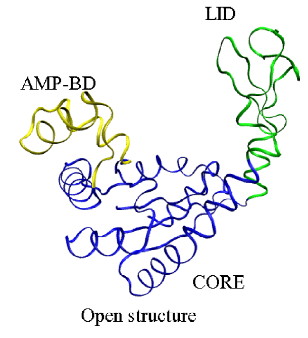
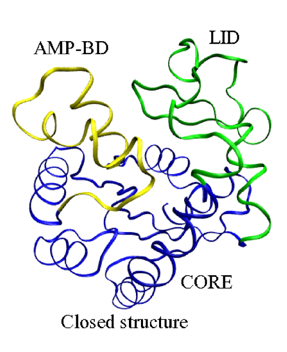
Figure 1: Crystal structures of adenylate kinase. The blue segment represents the core of the protein (CORE), the yellow segment is the AMP binding domain (BD), and the green segments is the flexible lid (LID). The top figure is the Apo (or Open) form, and the bottom figure is holo (Closed) form.

and thus helps to regulate the relative amounts of cellular energetic units.^{37, 38, 39} The crystal structure of Adk for E. coli is available in several conformations. Its native apo form (Protein Databank code 4AKE⁴⁰) is shown in Figure 1 (a). In the figure, the blue segments represent the core (CORE), the yellow segment represents the AMP binding domain (BD), and the green segment represents the flexible lid (LID). Upon ligand binding, the enzyme closes over the ligands. The crystal structure (1AKE)⁴¹ of the holo form of the enzyme obtained in complex with a ligand that mimics both AMP and ATP is shown in Figure 1 (b). Clearly, in the apo form, the enzyme shows an Open structure (that we denote as O in this manuscript), and in the holo form, it is Closed (denoted by C throughout).

Adk has been studied previously via computational methods using both coarse–grained models and fully atomistic simulations. Coarse–grained models used to study transition pathways for Adk have, primarily, utilized network models.^{34, 42, 35, 43} In these methods, the fluctuations in proteins are represented by harmonic potentials, and the deformations due to these fluctuations are used to estimate the free energy in the basins (end states and/or multiple basins). Subsequently, a minimum energy path is calculated to characterize the transition.

A few groups have also studied conformational fluctuations in Adk using atomistic models. In an interesting amalgamation of coarse and atomistic models, Arora and Brooks⁴⁴ performed atomistic (with implicit solvent) umbrella sampling molecular dynamics (MD) simulations along an initial minimum energy path suggested by a network model. Kubitzki and de Groot⁴⁵ performed replica exchange MD for atomistic Adk to increase conformational sampling of adenylate kinase – and observed both O and C conformers; however, a true path ensemble is not obtained from replica exchange. In other work, fully atomistic MD on the two end structures has been performed to observe fluctuations in the two ensembles^{37, 46} but direct conformational transitions were not observed.

In the present study, we use semi–atomistic models to improve chemical accuracy compared to typical coarse–grained models while still performing high quality path sampling. In our models, the backbone is fully atomistic to provide chemically realistic geometry. Inter–residue interactions are modeled at a coarse–grained level via the commonly used double–G$\bar{\mathrm{o}}$ potentials^{31, 47, 43, 48} that (meta)stabilize two crystal structures. Additionally, one of the models uses residue–specific interactions to probe the effect of such interactions. We use a library–based Monte Carlo (LBMC) scheme to perform sampling.⁴⁹. LBMC was previously developed in our group and shown to facilitate the use of semi–atomistic models of the type used here.⁴⁹

Transitions between the Open and the Closed states (both directions) are studied with the weighted–ensemble (WE) path–sampling method³³ that has been previously been studied to study folding of proteins,⁵⁰ protein dimerization,⁵¹ and conformational transitions in an alpha–carbon model of calmodulin.³² WE was shown to promote efficient path sampling of conformational transitions in purely alpha–carbon model of calmodulin.³² Additionally, WE is statistically exact: it preserves natural system dynamics, resulting in an unbiased path ensemble.⁵²

Biophysically, we focus on heterogeneity of the path ensemble (multiple pathways) and the forward–reverse “symmetry” of the ensemble. It is possible that evolution has favored the fine–tuned precision of a single pathway in some systems, but the “robustness” of alternative pathways in other cases. Although our semi–atomistic models preclude biochemically precise conclusions, our path sampling means that we can provide a complete description in a model system. Further, good path sampling enables us to investigate, perhaps for the first time, the issue of symmetry between forward and reverse transitions – which has implications for studies of protein unfolding.^{53, 54, 55}

The goal of this work, in summary, is to probe the biophysics of transitions with the most detailed models that allow for generating an ensemble of pathways. The manuscript is organized as follows. First, In Section 2 we discuss the models we use to depict the protein. Section 3 then describes the method to generate the ensemble of pathways. In Section 4, we present results for transitions in both the directions for all the three models we used. We discuss the results, efficiency, and future models in Section 5, with conclusions given in Section 6.

2 Semi–atomistic models

We use three semi–atomistic models, expanding on our previous work.⁴⁹ In all the models, the backbone is represented in full atomistic detail, using the three residues alanine, glycine, and proline.⁴⁹ All intraresidue interactions are included explicitly, using the OPLSAA all–atom force field. Both the intra–residue interaction energies and the configurations are stored in libraries as described previously.⁴⁹ In brief, we note that libraries of the three types of residues are pre–generated according to the Boltzmann distribution at 300 K, and alanine is used to represent the backbone of all residues besides glycine and proline (a simplification motivated by the similarity of Ramachandran maps for the residues).⁵⁶ Ligands are not modeled explicitly in this path sampling study.

The differences in the three models lie in the treatment of inter–residue interactions: two of the models use only double–G$\bar{\mathrm{o}}$ interactions at backbone alpha carbons, whereas one model uses both double–G$\bar{\mathrm{o}}$ and residue–specific interactions. Complete information is given below.

All three semi–atomistic models employ double–G$\bar{\mathrm{o}}$ interactions. Following Ref ³¹, for each of the two crystal structures, residues pairs with alpha carbons less than 8 $\mathrm{\AA}$ apart are considered native contacts. In the G$\bar{\mathrm{o}}$ energy of an arbitrary configuration, every native contact from the Open form is assigned an energy of $-\epsilon$, whereas those exclusively found in the Closed form are scaled to be $-e_{\mathrm{scale}}\epsilon$. G$\bar{\mathrm{o}}$ interactions do not distinguish between different types of residues except in terms of size. This double–G$\bar{\mathrm{o}}$ potential between two residues $i$ and $j$ with alpha carbon distance $r_{ij}$ is given by

$$u^{\mathrm{G\bar{o}}}(r_{ij})=\begin{cases}\infty,&r_{ij}<r_{ij}^{\mathrm{X}}(1-\delta)\\ -\epsilon_{\mathrm{X}},&r_{ij}^{\mathrm{X}}(1-\delta)\leq r_{ij}<r_{ij}^{\mathrm{X}}(1+\delta)\\ 0.3\epsilon,&r_{ij}^{\mathrm{X}}(1+\delta)\leq r_{ij}<r_{ij}^{\mathrm{Y}}(1+\delta)\\ -\epsilon_{\mathrm{Y}},&(\ast)r_{ij}^{\mathrm{Y}}(1-\delta)\leq r_{ij}<r_{ij}^{\mathrm{Y}}(1+\delta)\\ 0,&r_{ij}\geq r_{ij}^{\mathrm{Y}}(1+\delta)\end{cases}$$ (2)

where $r_{ij}^{\mathrm{X}}$ and $r_{ij}^{\mathrm{Y}}$ are the native distances in the two crystal structure ordered such that $r_{ij}^{\mathrm{X}}<r_{ij}^{\mathrm{Y}}$ (X and Y equate to Open or Closed), and $\delta$ is a well–width parameter chosen to be 0.05. If X equals Open and Y equals Closed, $\epsilon_{\mathrm{X}}=\epsilon$ and $\epsilon_{\mathrm{Y}}=e_{\mathrm{scale}}\epsilon$, and vice–versa. In the case of overlapping square wells, $r_{ij}^{\mathrm{X}}(1+\delta)>r_{ij}^{\mathrm{Y}}(1-\delta)$, the $0.3\epsilon$ barrier in the middle does not exist and the lower limit of the inequality marked with $(\ast)$ is replaced by $r_{ij}^{\mathrm{X}}(1+\delta)$.

The total G$\bar{\mathrm{o}}$ interactions are therefore

$$U_{{\mathrm{G}}\bar{\mathrm{o}}}(e_{\mathrm{scale}})=\sum_{i<j}u^{{\mathrm{G}}\bar{\mathrm{o}}}(r_{ij}).$$ (3)

For Model 1, we have

$$U_{1}=U_{\mathrm{G\bar{o}}}(e_{\mathrm{scale}}=1).$$ (4)

The motivation behind using such a double G$\bar{\mathrm{o}}$ potential is that the two “end” crystal structures are presumed stable – and the double–G$\bar{\mathrm{o}}$ protocol guarantees that bistability. Such double G$\bar{\mathrm{o}}$ interactions have been used to probe the biophysics of several systems.^{31, 47, 43, 48}

2.1 Model 1: Pure double G$\bar{\mathrm{o}}$ with energy symmetry

Previous path sampling studies of proteins were limited to smaller systems and/or simpler models. We, therefore, first study whether the simplest model within the semi–atomistic framework can be fully path sampled. Our Model 1 omits most chemical details and uses only symmetric double–G$\bar{\mathrm{o}}$ interactions as given in eq 3. That is, native contacts in the Open and the Closed structure are treated identically ($e_{\mathrm{scale}}=1$).

Because Model 1 is a pure G$\bar{\mathrm{o}}$ model, the temperature is specified in units of the well depth of G$\bar{\mathrm{o}}$ interactions, $\epsilon$. We choose the temperature as the highest at which the two experimental crystal structures are stable. We therefore performed a series of Monte Carlo simulations, as described below, at various temperatures. At $T=0.75\epsilon/k_{\mathrm{B}}$, both structures melted, but both remained (meta)stable at $T=0.7\epsilon/k_{\mathrm{B}}$. Thus, for Model 1, all subsequent equilibrium and path sampling simulations were performed at $T=0.7\epsilon/k_{\mathrm{B}}$.

2.2 Model 2: Double G$\bar{\mathrm{o}}$ with residue–specific interactions

Our second model adds chemical detail, both to improve upon the simplicity of Model 1, and to provide a way to check the sensitivity of our results to modeling choices. Model 2 includes atomistic backbone hydrogen bonding, Ramachandran propensities, and residue–specific contact interactions, as detailed below. Because these interactions are implemented as short ranged, Model 2 is only about 30$\%$ slower than Model 1, based on wall–clock time per MC step. G$\bar{\mathrm{o}}$ interactions are again symmetric, with $e_{\mathrm{scale}}=1$.

Our semi–atomistic LBMC platform makes the inclusion of additional interactions straightforward. Since the backbone is modeled atomistically, backbone–backbone hydrogen bonding is easily incorporated, as described below. However, due to the absence of explicit side chains in the present implementation, residue–specific chemical interactions can only be incorporated at a coarse–grained level. We use residue–specific contact interactions based on the work of Miyazawa and Jernigan (MJ),^{57, 58} as discussed below. Specifically, we use the potential energy

$$U_{2}=U_{\mathrm{G\bar{o}}}(e_{\mathrm{scale}}=1)+U_{\mathrm{HB}}+U_{\mathrm{Rama}}+U_{\mathrm{MJ}}$$ (5)

where $U_{\mathrm{HB}}$ is the hydrogen–bonding potential, $U_{\mathrm{Rama}}$ is the potential due to Ramachandran propensities, and $U_{\mathrm{MJ}}$ is the residue–specific potential based on MJ interactions. These terms are described below.

Hydrogen bonding for the backbone–backbone interactions is modeled atomistically, but with simplifications appropriate to the otherwise coarse–grained nature of our models. Specifically, we use ordinary Coulomb interactions with OPLSAA charges between the backbone CO and NH groups if the O–H distance less than 2.5 $\mathrm{\AA}$. The cutoff was chosen as the distance after which dipole interactions are significantly attenuated. Following previous studies that suggest a dielectric constant of 2–5 inside a protein, we use a value of 3. The use of physical charge and distance units in the hydrogen–bonding interactions allows physical temperature units in the simulation (instead of merely being in relation to the G$\bar{\mathrm{o}}$ well depth).

Ramachandran propensities were included via the term $U_{\mathrm{Rama}}$, which is based on a potential of mean force obtained by calculating the distribution of $\Phi$–$\Psi$ dihedral angles in acetaldehyde–alanine–n–methylamide using OPLSAA force field. This distribution was tabulated from a Langevin dynamics simulation at 300 K using the GBSA implicit solvent model in Tinker software package.

The construction of MJ–type interactions required some care. Several variants of the original MJ interaction values have been utilized in the literature (such as scaling the MJ interactions energies, as well as shifting)^{59, 60} – due to the fact that MJ values are based on folded protein data and are not directly applicable for unfolded states. We follow the suggestion of Jernigan and Bahar⁵⁹ to mix MJ values of Table V and Table VI (numbering as in the original MJ paper,⁵⁷ with updated values as in Ref ⁵⁸) so that the residue specific interactions are modeled as $x\times$(Table V)$+(1-x)\times$(Table VI). We chose $x=0.05$ to ensure that the residue–specific interactions are a significant perturbation of the double G$\bar{\mathrm{o}}$ interactions.

To make the crystal structures (meta)stable, we “titrated in” double G$\bar{\mathrm{o}}$ interactions ($\epsilon$), until bistability was observed at 300 K. Because, as described, hydrogen bonding introduces physical units into Model 2, the units of G$\bar{\mathrm{o}}$ well depth, $\epsilon$, are also physical. We found that at $\epsilon/k=400$ K, both the structures remained (meta)stable.

2.3 Model 3: Pure double G$\bar{\mathrm{o}}$ without energy symmetry

Finally, to facilitate the generation of large path ensembles in both the Open–to–Closed and Closed–to–Open directions, we also constructed a third model. The new model is designed to overcome the somewhat artifactual over–stabilization of the Closed states in Models 1 and 2 (see results below in Section 4). In brief, our 8 $\mathrm{\AA}$ cutoff permits significantly more contacts in the Closed state, implicitly but artificially mimicking the presence of ligands in Models 1 and 2. This implicit presence of ligands interferes somewhat with our goal of modeling the ligand–free opening and closing of the enzyme.

In Model 3, therefore, we attempt to make the Open and Closed forms of adenylate kinase more comparable in stability. We decrease the strength of G$\bar{\mathrm{o}}$ interactions specific to the Closed form to half of G$\bar{\mathrm{o}}$ interactions (i.e., we set $e_{\mathrm{scale}}=0.5$). Additionally, to focus on the effect of the reduced stability of the Closed form with respect to the Open form, we use only asymmetric double G$\bar{\mathrm{o}}$ interactions (and no H-bonding, Ramachandran, or MJ interactions). That is, we set

$$U_{3}=U_{\mathrm{G\bar{o}}}(e_{\mathrm{scale}}=0.5).$$ (6)

3 Methods

3.1 Dynamical Monte Carlo

We follow many precedents^{61, 62, bin1} and use “dynamical” MC for the dynamics of our models. Such an approximation to physical dynamics is consistent with our use of simplified models. Specifically, we use the library–based Monte Carlo (LBMC) algorithm,⁴⁹ to propagate the system in both brute–force simulations for generating equilibrium ensembles and path sampling simulations (discussed below in more detail). For both equilibrium and path sampling, the systems always evolve via “natural” LBMC dynamics, and no artificial forces are used to direct conformational transitions, as explained below.

Our LBMC simulations use the same trial moves described in our earlier work.⁴⁹. Namely, one flexible peptide plane in the current configuration is swapped with one stored in the library, and a $\Psi$ angle is also displaced by a small amount.

3.2 Path sampling

In systems with rugged energy landscapes, such as proteins, regular brute–force simulations are not efficient for studying transitions. For this reason, we use the statistically rigorous weighted–ensemble (WE) path sampling method to generate path ensembles of conformational transitions of adenylate kinase between the Open and the Closed states. This method preserves the natural system dynamics⁵² and was used previously to study protein folding,⁵⁰, protein dimerization,⁵¹, and conformational transitions of calmodulin using an alpha–carbon model.³² Weighted ensemble studies the probability evolution of trajectories in the configuration space using any underlying system dynamics.⁵² In this work, we use the WE method to study transitions in more detailed models to evaluate the effect of increasing chemical detail on the transitions, and to study questions of symmetry in forward and reverse directions.

The procedure to use weighted–ensemble path sampling to study conformational transitions is described in detail elsewhere,^{33, 32, 52} and here we describe our simple implementation briefly. Prior to beginning the simulations, we divide a one dimensional projection of the configurational space (i.e., the DRMS from the target structure in the present study) into a number of bins. The DRMS is a “progress coordinate” or “order parameter” – and is not necessarily the reaction coordinate. The progress coordinate roughly keeps track of the progress to the target state: the DRMS of structures close to the target state is necessarily small. It is also possible to use multidimensional or adaptively changing progress coordinates,^{32, 52} but was not found necessary here.

In the weighted–ensemble method, an evolving set of trajectories and their probabilities are tracked. Procedurally, several independent trajectories are started in an initial configuration and run for a short time interval $\tau$ (consisting of multiple simulation steps) with natural dynamics. At the end of each $\tau$ interval, the progress of the trajectories along the progress coordinate is noted (i.e., into which bin along the progress coordinate each trajectory ends). Once bins are tabulated after each $\tau$, trajectories are “split” (replicated with divided probability) and combined. This keeps the same number of trajectories in each occupied bin, prunes low–weight trajectories and splits trajectories with high probability. This splitting and combining of simulations is performed statistically as discussed elsewhere.^{33, 32, 52} The probability remains normalized and all probability flows can be measured.

The full details of our WE simulations are as follows. We employ LBMC to describe the natural system dynamics. We utilize 25 bins between the two states, with 20 simulations (trajectories) in each occupied bin. The end state is defined as being at a DRMS of 1.5 $\mathrm{\AA}$ from the target crystal structure, a definition used in both directions. Using this definition of the end state, we calculate the probability flux of trajectories entering the target state at the end of each $\tau$.

It should be noted that value of the probability flux into either state – and hence the rate – depends upon the precise definitions of the two states. Although probability flows are good indicators of sampling quality, precise numerical values of the rates are not of great interest in our study of simple models with Monte Carlo dynamics. In this work, we are interested in the path ensembles and not the rates.

4 Results

4.1 Static analysis of conformational differences

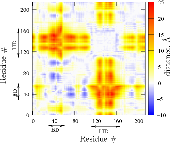
Figure 2: Map of the difference in the inter–residue distances of the Open from the Closed crystal structure. The map is, by definition, symmetric about the diagonal. The white space on the diagonal just implies that we do not calculate distances between residue pairs less than 2 residues apart along the chain. The residues corresponding to the LID and BD are labeled and the unlabeled residues form the CORE.

For reference, we first analyze the conformational differences between the two end–state static crystal structures to quantify the observed differences in the Open and Closed configurations of Figures 1. Figure 2 shows the $\alpha$–carbon distance difference map of pairs of residues in the Open and the Closed crystal structures. A large positive value implies that a pair is farther apart in the Open structure than in the Closed structure, whereas a negative value is the opposite. By construction, the figure is symmetric about the diagonal. A few features of the two structures easily emerge from Figure 2. The inter–residue distances for most of the residue pairs are very similar in the two crystal structures. The major differences are that the distances in the Closed structure between residues labeled LID (114–164) are closer to BD (31–60) and several residues of CORE are smaller than the corresponding distances in the Open structure. Thus, Figure 2 quantifies Figure 1.

From Figures 1 and 2 it is clear that the structural change that characterizes the transition between the Open and the Closed structure is fairly straightforward: the LID and the BD close, and the rest of the protein remains fairly unchanged. Following Figures 1 and 2, for the path sampling studies presented shortly, we monitor inter–residue distances between two pairs of residues: residues 56 (GLY) and 163 (THR), which report on the BD–LID proximity, as well as residues 15 (THR) and 132 (VAL), which report on the CORE–LID proximity. In the Closed structure, $d_{56,163}^{\mathrm{c}}=4.9\mathrm{\AA}$ and $d_{15,132}^{\mathrm{c}}=6.3\mathrm{\AA}$. On the other hand, in the Open structure, $d_{56,163}^{\mathrm{o}}=23.6\mathrm{\AA}$ and $d_{15,132}^{\mathrm{o}}=17.8\mathrm{\AA}$. Thus, the relation between the CORE and LID is monitored, along with that of the LID and BD.

4.2 Brute force equilibrium sampling

In order to demarcate the native basins in our analysis of transitions, we first study equilibrium ensembles for the Open and the Closed states of adenylate kinase. Put another way, we want to quantify the size of native–basin fluctuations in our models. Further, we determine whether transition paths can be obtained without the aid of path sampling.

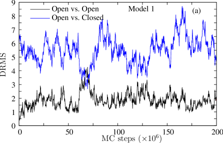
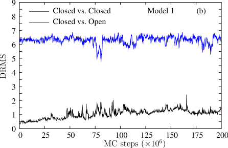
Figure 3: Stability of the native basins in Model 1. The DRMS in Model 1 (pure G$\bar{\mathrm{o}}$) is shown for two simulations (a) starting from the Open structure and (b) starting from the Closed structure. For each simulation, we show the DRMS from the starting structure (black line) and the opposing structure (blue line). Neither simulation show a transition to the opposing structure, but the scales of fluctuations are very different.

We quantify fluctuations in the equilibrium ensembles in the two basins by using DRMS from the respective crystal structures. Figure 3 (a) shows two sets of DRMS traces for Model 1 for a simulation started from the Open structure: DRMS–from–Open (black line) and DRMS–from–Closed (blue line). Similarly, Figure 3 (b) shows two sets of DRMS traces for Model 1 for a simulation started from the Closed structure: DRMS–from–Closed (black line) and DRMS–from–Open (blue line). Thus, in each panel, the black line represents DRMS from the starting structure, whereas the blue line represents DRMS from the opposing structure.

A comparison of the two panels of Figure 3 shows that the simulation started from the Open structure shows significantly more fluctuations than the simulation started from the Closed structure. Furthermore, the fluctuations drive the simulation started from the Open structure closer to the Closed structure than vice versa. For example, Figure 3 (a) shows that the simulation started from the Open structure gets to within 3 $\mathrm{\AA}$ of the Closed structure at approximately 70 million MC steps. On the other hand, the simulation started from the Closed structure (Figure 3 (b)) remains farther from the Open structure.

Most importantly, neither simulation show a transition to the opposing structure. The DRMS from the opposing structure for a particular simulation is always significantly larger than DRMS values from the starting structure for the other simulation. To elaborate, let us consider the DRMS–vs–Closed structure for the simulation started from the Closed structure (black line in Figure 3 (b)). The fluctuations in DRMS remain less than 1.5 $\mathrm{\AA}$ in the native basin for the Closed structure. Comparatively, the largest fluctuations in the simulations started from the Open structure bring it only within at most 3 $\mathrm{\AA}$ of the Closed structure (blue line in Figure 3 (a)). That is, the opposing native basin is never reached.

We mention that all the DRMS values plotted in Figures 3 (a) and (b) are based on the first 200 residues. This is because the 14 tail residues, which form a helical segment, are very flexible and the helix unravels in either structure at a much lower temperature than the stable part of the protein. Thus, Figure 3 focuses on the rest of the protein. Additionally, although we show results for $T=0.7$ here, simulations at lower temperatures also give qualitatively similar results.

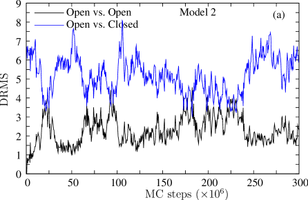
Figure 4: Stability of the native basins in Model 2. The DRMS in Model 2 (G$\bar{\mathrm{o}}$, H-bonding, Ramachandran propensities, and MJ–type residue specific interactions) is shown for two simulations (a) starting from the Open structure and (b) starting from the Closed structure. For each simulation, we show the DRMS from the starting structure (black line) and the opposing structure (blue line). Neither simulation show a transition to the opposing structure, but the scales of fluctuations are very different.

We perform an analogous fluctuation analysis for Model 2 which incorporates backbone hydrogen bonding interactions, Ramachandran propensities, and some residue specificity via MJ–type interactions. Figure 4 (a) shows the DRMS (of the first 200 residues) from the Open (black line) and Closed (blue line) structures for a simulation started from the Open structure. Similarly, Figure 4 (b) shows the DRMS traces for a simulation started from the Closed structure. Again, we observe very similar results as for Model 1: the fluctuations in the Open ensemble are larger than in the Closed ensemble, and no transition to the opposing structure is obtained in either simulation.

4.3 Path sampling: Models 1 and 2

Due to the inability of brute–force simulations to show transitions, we use weighted–ensemble path sampling to generate an ensemble of transition pathways with the aim of assessing path heterogeneity. In particular, we examine transitions in both directions for all the three models.

4.3.1 Transition from Open to Closed State

We first check whether our path sampling is sufficient by monitoring the flux into the target state. Figure 5 plots the WE results for probability fluxes obtained into the Closed state for both Models 1 and 2. The “time” axis is merely the number of $\tau$ intervals (where one interval contains 2000 LBMC steps). In both models, the fluxes reach linear regimes indicating that the observed transitions are not merely due to initial fast trajectories and the path ensemble is appropriately sampled.

The sensitivity to the models is also apparent in the fluxes shown in Figure 5: Model 2 (which includes hydrogen–bonding, Ramachandran propensities, and MJ–type residue specific interactions) has a smaller flux into the Closed state than Model 1. Residue–specific interactions are expected to roughen the energy landscape, consistent with the observed slowing of transition dynamics. However, the possible change in the Open state basin stability due to addition of these interactions is convoluted with the roughening of the landscape.

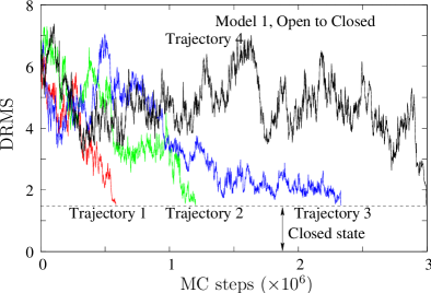
Figure 6: Open–to–Closed transitions observed for Model 1. Four typical DRMS traces are shown, measured from the Closed crystal structure. The Closed basin is delimited by a DRMS of 1.5 $\mathrm{\AA}$ from the Closed crystal structure.

We further study the path ensemble by examining individual trajectories. Figure 6 shows, for Model 1, the DRMS from the Closed structure for four typical transitions started in the Open state as a function of time (total number of LBMC steps) obtained via WE path sampling. In contrast with the brute–force simulation in Figure 3 (a), each trajectory in Figure 6 gets to the Closed state (defined to be within a DRMS of 1.5 $\mathrm{\AA}$ from the Closed structure). Although the trajectories arrive at the target state with different weights, the ones shown in the figures above are obtained after a simple resampling procedure,⁶³ and, thus, represent trajectories that arrive with relatively large probabilities. Resampling is a statistically rigorous procedure to prune an ensemble.⁶³ In our resampling scheme, a trajectory arriving at the target with weight $w$ is kept with a probability $w/w_{\mathrm{max}}$.

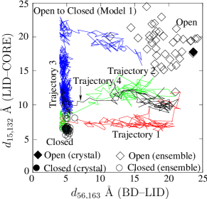
Figure 7: Path heterogeneity in Model 1 transitions. Four typical trajectories for the Open–to–Closed transition (Figure 6 are shown via distances between the CORE and LID (ordinate) and between the BD and the LID (abscissa). The “dwell” times for the trajectories in the Open state excluded for clarity.

For trajectories that begin transitions at larger times (such as Trajectory 4 in Figure 6), a significant amount of time is spent in regions with large DRMS values from the Closed structure. Thus, in Figure 7 and beyond, we do not show the “dwell time” in the Open state.

To analyze the order of domain closing, and, in particular, to study possible heterogeneity in the path ensemble, we study the four trajectories of Figure 6 in more detail. Figure 7 plots the projection of the above four trajectories onto the $d_{15,132}$ and $d_{56,163}$ plane (see Section 4.1) obtained via WE for Open–to–Closed transition. The filled circle shows the Closed x–ray structure, whereas the filled diamond is for the Open x–ray structure. The corresponding open circles and diamonds are representative of fluctuations in the ensembles of Closed and Open structures, respectively. The relatively larger spread of structures in the Open ensemble compared to Closed reflects the larger Open–state fluctuations depicted previously in Figure 3. The four different colored lines show the four trajectories of Figure 6, without the “dwell time” in the Open ensemble.

In all the trajectories, the transition through the region with values of $d_{56,163}$ (BD–LID distance) intermediate between the two ensembles is fairly rapid. The flexible LID undergoes large fluctuations in the Open state, and the transition to the Closed state is typically accomplished via the BD snapping closed on a much smaller timescale.

Despite the relatively fast closing of the BD for the trajectories in Figure 7, the exact transition paths traced by the four trajectories are significantly different. For Trajectory 1, the BD shuts after the flexible LID gets close to the CORE. For the following discussion, we call this pathway as Open–LID–BD–Closed (first the LID relaxes, and then the BD shuts close). On the other hand, Trajectory 3 shows a dramatically different behavior: the BD snaps shut before the flexible LID gets closer to the CORE (this pathway is labeled as Open–BD–LID–Closed). The other two trajectories are somewhere in between the two extremes.

To quantify heterogeneity in the path ensembles, we compare the ratio of trajectories in the two transition pathways. Specifically, we define a trajectory to follow the Open–LID–BD–Closed (lower right) pathway if it first visits the region $d_{56,163}<10.0$ $\mathrm{\AA}$ after last leaving the rectangular Open–state region defined by $d_{56,163}>10.0$ $\mathrm{\AA}$ and $d_{15,132}>10.0$ $\mathrm{\AA}$. On the other hand, a trajectory follows the Open–BD–LID–Closed (upper left) pathway if it first visits the region $d_{56,163}>10.0$ $\mathrm{\AA}$ after last leaving the above Open–state rectangular region. We find that for Open–to–Closed transition using Model 1, approximately 60$\%$ of the resampled trajectories follow Open–BD–LID–Closed pathway (akin to Trajectory 3 in Figure 7). The remaining 40$\%$ follow the Open–LID–BD–Closed pathway.

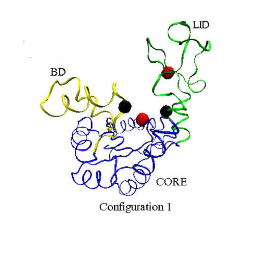
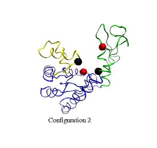
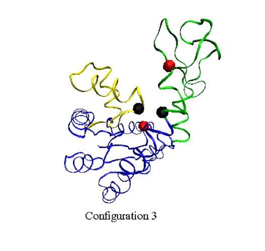
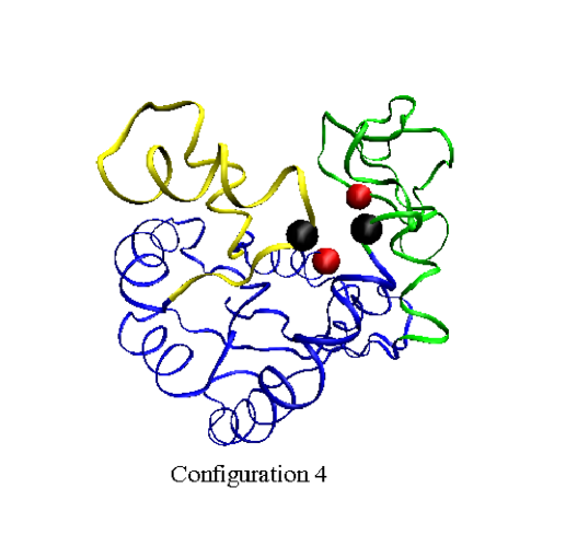
Figure 8: Four time–ordered, representative structures along the Open–BD–LID–Closed path obtained for Trajectory 3 in Figure 7 (Model 1). The CORE domain is blue, the BD is yellow, and the LID is green. The configurations correspond to (296000, 802000, 822000, 1496000) MC steps, respectively, in Trajectory 3 of Figure 6.

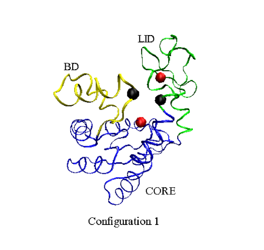
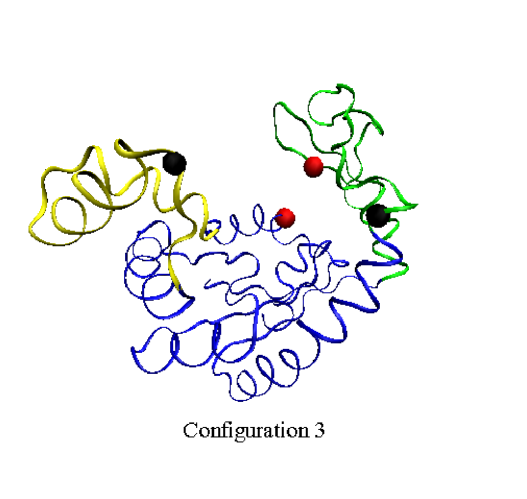
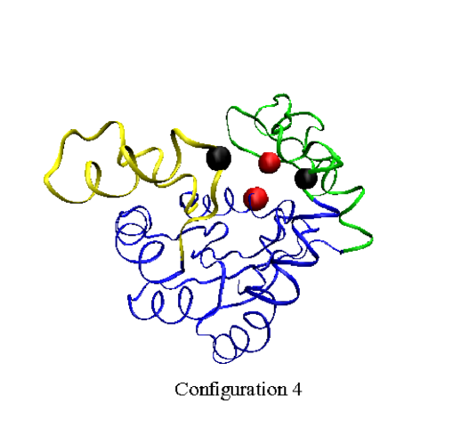
Figure 9: Four time–ordered, representative structures along the Open–LID–BD–Closed path obtained for Trajectory 1 in Figure 7 (Model 1). The CORE domain is blue, the BD is yellow, and the LID is green. The configurations correspond to (128000, 206000, 306000, 480000) MC steps, respectively, in Trajectory 1 of Figure 6.

Further, we look at a few intermediate structures for these two pathways. Figure 8 shows four intermediates along Trajectory 3 of Figure 7. The BD and LID domains near one another before the LID closes. On the other hand, Figure 9 shows four intermediates along Trajectory 1 in Figure 7. The closing of the LID, followed by snapping shut of the BD is clearly visible in the figure. As both Figures 8 and 9 show, the rest of the protein (i.e., the CORE region) maintains a stable shape during the transformation.

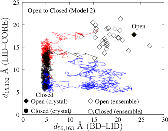
Figure 10: Path heterogeneity depicted via four typical trajectories for the Open–to–Closed transition obtained using Model 2 shown via distance between the CORE and LID (ordinate) versus the distance between the BD and the LID (abscissa). The “dwell” times for the trajectories in the Open state excluded for clarity.

To determine the sensitivity of the path ensemble to the model, we similarly analyzed results from Model 2 (which includes hydrogen bonding, Ramachandran propensities, and a level of residue specificity). A similar qualitative picture is obtained for Model 2. Figure 10 plots three of the resampled trajectories from the Open to the Closed structure using Model 2. The “dwell times” in the Open state have been omitted for clarity. Again, the symbols have the same meaning as in Figure 7 (except that open symbols represent the fluctuations obtained using Model 2). The transition from the Open–to–Closed structure primarily takes place by the BD snapping closed to the LID on a much shorter time scale. Depending upon the relative positions of the LID and CORE, the completion of the transition requires further adjustment of the LID relative to the CORE. The ratio of paths in the two pathways is the same as that for Model 1.

4.3.2 Transition from Closed to Open State

We also studied “reverse” transitions – from the Closed to the Open state. Figure 11 shows the flux into C as a function of “time” for both Models 1 and 2. Compared to Figure 5 for the transition from the Open to the Closed state, the flux into state B is several orders of magnitude lower. This observation mirrors the previously described larger fluctuations in the Open state ensemble. Flux into the Open state for Model 2 with residue specific chemistry is higher than for Model 1, despite the expected roughening of the energy landscape. This necessarily reflects a free energy shift, suggesting MJ interactions de–stabilize the Closed state compared to a pure double–G$\bar{\mathrm{o}}$ model. Such a shift seems appropriate given that we do not model ligands which implicitly lead to more contacts in the Closed state and consequent over–stabilization in the G$\bar{\mathrm{o}}$ model.

For Closed–to–Open transition using either model, we obtain pathways which mirror the Open–to–Closed transition: the LID fluctuates in the Closed state, and this is followed by the BD snapping open on a relatively fast time scale. For both Models 1 and 2, successful trajectories appear to follow only the Closed–LID–BD–Open pathway for Closed–to–Open transition (reverse order of the Open–BD–LID–Closed pathway in the Open–to–Closed transition direction). The absence of symmetry is surprising given our recent formal demonstration,³⁶ and there seem to be two possible reasons. First, the transients for Closed–BD–LID–Open pathway are long–lived. Lengthy transients are consistent with the low reverse reaction rates, shown in Figure 11, for both Models 1 and 2. Second, our state definitions may be flawed as discussed in Section 5.2.

To clarify the issue of the symmetry of path ensembles between forward and reverse directions, we constructed and path sampled Model 3.

4.4 Path ensemble symmetry analysis in Model 3

The slow Closed–to–Open transitions indicates that, for Models 1 and 2, the free energy of the Closed structure is significantly lower than that of the Open structure. As discussed in Section 2.3, this suggested the use of Model 3, which decreases in magnitude the favorable energy for contacts present only in the Closed state. That is, Model 3 reduces the free energy asymmetry between the Open/Closed states.

Model 3 thereby facilitates study of the symmetry between forward and reverse transitions. As shown in Figure 12, although the flux in the Open–to–Closed direction in Model 3 is higher than in the Closed–to–Open direction, the difference between the fluxes in the two directions is much less than that for Models 1 and 2. The increased Closed–to–Open rate implies that the relative stability of the Closed state is reduced compared to Models 1 and 2. Importantly, the relatively linear behavior of fluxes in both the directions implies our path sampling is sufficient – well beyond transients.

For Model 3, we examine the same classification of pathways as above. Both paths are frequently observed in both directions. In Figure 13, we show the ratio of probabilities of the two paths as a functions of simulation time in the two directions. Values in each window are averaged over 500 $\tau$ increments. The results for the Open–to–Closed direction (diamonds) are shown for a single simulation, whereas the Closed–to–Open transitions (circles) are shown for 6 independent simulations. Despite large fluctuations, the ratios of paths in the two directions are similar. We discuss the issue of path symmetry further, below.

5 Discussion

5.1 Models

An important issue in any coarse–grained study is the sensitivity of the results to the particular model(s) used. To address this point, we used three different semi–atomistic models of adenylate kinase. For the models used, we find that the transition pathways are not significantly affected by the models we used. In particular, we find two dominant pathways (Open–LID–BD–Closed and Open–BD–LID–Closed) that occur in all the models. Although the rates vary considerably among models, we do not expect realistic kinetics in simplified models.

Our choice of models was governed by the basic requirement of obtaining full path sampling of conformational transitions – in order to study path ensembles, heterogeneity, and symmetry. Two of the models are based purely on structure (G$\bar{\mathrm{o}}$ model) and the other (Model 2) includes some level of residue specificity via Miyajawa–Jernigan interactions, as well as hydrogen bonding energies and Ramachandran propensities. In Model 2, the chemical energy terms are significant perturbations to the G$\bar{\mathrm{o}}$ interactions. (as quantified by MJ interactions between residues). This model is designed to be able to capture a minimum level of biochemistry. However, Model 2 still requires significant G$\bar{\mathrm{o}}$–type interactions to stabilize the two physical states. In the future, we plan to utilize more detailed and explicit side chain–side chain and side chain–backbone interactions to reduce the dependence on G$\bar{\mathrm{o}}$–type interactions.

Another limitation is that we did not consider the ligand in our path sampling simulations. The inclusion of ligand could influence the observed pathways significantly. We have plans for modeling ligand via “mixed models” that include all–atom ligands and binding sites, with a coarse–grained picture for the rest of the protein. Such an explicit inclusion of ligands, with the corresponding degrees of freedom of the unbound ligands in the Open form should reduce the dependence on arbitrary G$\bar{\mathrm{o}}$ interactions. A study with explicit ligands could require a higher dimensional progress coordinates to use in weighted ensemble simulations: one coordinate for protein structure (as is done in this work), and a second (or further) coordinates for the distance between ligands and the protein. Note that weighted ensemble can mix real– and configurational–space coordinates: it was originally designed for binding studies.³³

5.2 Path symmetry

Recently, we investigate the conditions when there should be symmetry – i.e., when pathways in the forward and the reverse directions occur with the same ratio.³⁶ We show that exact symmetry will hold when a specific (equilibrium–based) steady state is enforced. Approximate symmetry is expected if the initial and final states are well–defined physical basins lacking slow internal timescales, so that trajectories emerging from a state “forget” the path by which they entered. Figure 13 suggests that the ratio of the two different pathways in the two directions is very similar for Model 3, which was fully path sampled in both directions.

Such a symmetry is clearly absent from our results (even after accounting for statistical fluctuations) in Models 1 and 2. Although we observed transitions in both the directions for all the models, Closed–to–Open transitions in all the models (especially in Models 1 and 2) are harder to obtain. In particular, the Closed–BD–LID–Open pathway is not observed in our simulations for Models 1 and 2. This indicates a lack of the correct steady state for these models in the Closed–to–Open direction and/or insufficiently well–defined states. It is unlikely that the highly flexible Open state is a good physical basin. We are currently working on developing WE path sampling methods that allow steady states to be sampled directly and efficiently.⁶⁴ Related steady–state methods are already available.^{65, 66, 67}

5.3 CPU time and efficiency

One of the basic goals of this work was to determine the level of detail we can include in a model, while still allowing for full sampling of the path ensemble. Thus, we now discuss the computational effort that was required. All simulations were performed on single 3 GHz Intel processors. The results shown for Model 1 in the Open–to–Closed direction took approximately one week of single CPU time. More simulation was performed in the Closed–to–Open direction, requiring 3-4 weeks of single CPU time. The results for Model 2 were obtained using approximately the same time as Model 1. For Model 3, the Closed–to–Open transition was not much harder to obtain than the Open–to–Closed transition, and a simulation in each direction required approximately two weeks of single CPU time. Due to the low CPU usage for obtaining path ensembles for the models used here, obtaining path ensembles of better models using WE is possible. See Section 5.1.

It is not hard to estimate the efficiency of WE simulation compared to brute–force. The transition rates determined from WE simulations indicate the time required for brute–force simulations to achieve transitions and hence permit estimates of efficiency. For example, the rate obtained for Closed–to–Open transition for Model 3 is 2.5$\times 10^{-6}/\tau$. Thus, one brute–force transition can be estimated to require the reciprocal amount of time. Since 2000$\tau$ require approximately one week of computing, BF is estimated to take approximately 4 years for a single transition. In contrast WE yielded 50 transitions after resemapling (i.e., 50 transitions with equal weights), in about two weeks of single–processor computing. (Before resampling, there were about 3000 WE transitions for each simulation). WE is thus significantly more efficient than BF. For transitions in the other direction and/or other models, a qualitatively similar picture for efficiency emerges.

6 Conclusions

We applied weighted ensemble (WE) path sampling to generate ensembles for conformational transition between Open (apo) and Closed (holo) forms of adenylate kinase using semi–atomistic models of the protein. No additional driving force was used to enable the transitions. We showed that conformational transitions in both directions are possible for such models via WE. In contrast, brute–force simulations are vastly inefficient. Given the relatively small computational effort required for observing transitions using WE, more detailed models can be used for full path sampling. In the future, models with further reduced dependence on G$\bar{\mathrm{o}}$–type interactions are needed, along with ligand modeling, to study the specific enzyme biochemistry – and path sampling of such models appears possible.

All the models show significant hereteogeneity in the transition pathways. In particular, two dominant pathways observed are characterized by the order in which the flexible lid and the AMP binding domains close. Although the rates obtained (in terms of Monte Carlo steps) varied significantly depending upon the model used, similar dominant pathways are obtained across the models. We further showed in the Appendix the formally exact result that the transition paths must be symmetric in the two directions in the (equilibrium–based) steady states. The model that allows significant transitions in both the directions shows an approximate symmetry which appears to be consistent with conditions on the symmetry rule.

Acknowledgments: We thank Dr. Bin Zhang and Prof. David Jasnow for helpful discussions. This work was supported by the NIH (Grant GM070987) and the NSF (Grant MCB–0643456).

Figure 5: Comparison of the probability fluxes into the Closed state for two models. The fluxes from a pure double–G$\bar{\mathrm{o}}$ system (Model 1, solid line) and a system with considerable chemical specificity (Model 2, dashed line) are plotted as functions of WE time intervals (each $\tau$ interval is 2000 LBMC steps). In both cases, the fluxes reach approximately linear regimes, suggesting transient effects have attenuated.

Figure 11: A comparison of probability fluxes into the Open state for two models as a function of WE time increment (each $\tau$ is 2000 LBMC steps). The solid line is for Model 1, whereas the dashed line is for Model 2. The log scale emphasizes the small amount of flux in Closed–to–Open direction for both the models, as compared to fluxes in the reverse direction.

Figure 12: Probability flux in either direction for Model 3 as a function of WE time increment (each $\tau$ is 2000 LBMC steps). For this model, the Closed–to–Open flux is of the same order of magnitude as in the reverse direction.

Figure 13: Ratio of probabilities of the two paths, 1 and 2, in the Open–to–Closed (diamonds) and Closed–to–Open directions (circles). Results from six independent WE simulations are shown in the Closed–to–Open direction to highlight the fluctuations. All data points are window averaged for 500 $\tau$.

References

- 1 Berg, J. M., L. Stryer, and J. L. Tymoczko. 2002. Biochemistry. Freeman, New York.
- 2 Hammes, G. G. 2002. Multiple conformational changes in enzyme catalysis. Biochem. 41:8221–8228.
- 3 Dellago, C., P. G. Bolhuis, F. S. Csajka, and D. Chandler. 1998. Efficient transition path sampling: Application to lennard–jones cluster rearrangements. J. Chem. Phys. 108:1964–1977.
- 4 Bolhuis, P. G., D. Chandler, C. Dellago, and P. L. Geissler. 2002. Transition path sampling: Throwing ropes over rough mountain passes, in the dark. Annu. Rev. Phys. Chem. 53:291–318.
- 5 van Erp, T. S., D. Moroni, and P. G. Bolhuis. 2003. A novel path sampling method for the calculation of rate constants. J. Chem. Phys. 118:7762.
- 6 van Erp, T. S., and P. G. Bolhuis. 2005. Elaborating transition interface sampling methods. J. Comp. Phys. 205:157–181.
- 7 Faradjian, A. K., and R. Elber. 2004. Computing time scales from reaction coordinates by milestoning. J. Chem. Phys. 120:10880–10889.
- 8 West, A. M. A., R. Elber, and D. Shalloway. 2007. Extending molecular dynamics time scales with milestoning: Example of complex kinetics in a solvated peptide. J. Chem. Phys. 126:145104.
- 9 vanden Eijnden, W., M. Venturoli, G. Ciccotti, and R. Elber. 2008. On the assumptions underlying milestoning. J. Chem. Phys. 129:174102.
- 10 Allen, R. J., P. B. Warren, and P. R. ten Wolde. 2005. Sampling rare switching events in biochemical networks. Phys. Rev. Lett. 94:018104.
- 11 Allen, R. J., D. Frenkel, and P. R. ten Wolde. 2006. Simulating rare events in equilibrium or nonequilibrium stochastic systems. J. Chem. Phys. 124:024102.
- 12 Borrero, E. E., and F. A. Escobedo. 2007. Reaction coordinates and transition pathways of rare events via forward flux sampling. J. Chem. Phys. 127:164101.
- 13 Lyman, E., and D. M. Zuckerman. 2007. On the structural convergence of biomolecular simulations by determination of the effective sample size. J. Phys. Chem. B. 111:12876–12882.
- 14 Juraszek, J., and P. G. Bolhuis. 2008. Rate constant and reaction coordinate of trp–cage folding in explicit water. Biophys. J. 95:4246–4257.
- 15 Elber, R. 2007. A milestoning study of the kinetics of an allosteric transition: Atomically detailed simulations of deoxy scapharca hemoglobin. Biophys. J. 92:L85–L87.
- 16 Schlick, T., and O. Perisic. 2009. Mesoscale simulations of two nucleosome–repeat length oligonucleosomes. Phys. Chem. Chem. Phys. 11:10729–10737.
- 17 Hu, J., A. Ma, and A. R. Dinner. 2006. Bias annealing: A method for obtaining transition paths de novo. J. Chem. Phys. 125:114101.
- 18 Schlitter, J., M. Engels, P. Kruger, E. Jacoby, and A. Wollmer. 1993. Targeted molecular–dynamics simulation of conformational change – application to the t–r transition in insulin. Mol. Simul. 10:291–309.
- 19 Ma, J., and M. Karplus. 1997. Molecular switch in signal transduction: Reaction paths of the conformational changes in ras p21. Proc. Natl. Acad. Sci. 94:11905–11910.
- 20 Apostolakis, J., P. Ferrara, and A. Caflisch. 1999. Calculation of conformational transitions and barriers in solvated systems: Application to alanine dipeptide in water. J. Chem. Phys. 110:2099–2108.
- 21 Elber, R. 1987. A method for determining reaction paths in large molecules – application to myoglobin. Chem. Phys. Lett. 139:375.
- 22 Ulitsky, A. 1990. A new technique to calculate steepest descent paths in flexible polyatomic systems. J. Chem. Phys. 92:1519.
- 23 Fischer, S., and M. Karplus. 1992. Conjugate peak refinement – an algorithm for finding reaction paths and accurate transition states in systems with many degrees of freedom. Chem. Phys. Lett. 194:252.
- 24 Sevick, E. M., A. T. Bell, and D. N. Theodorou. 1993. J. Chem. Phys. 98:3196.
- 25 Gillilan, R. E., and K. R. Wilson. 1992. Shadowing, rare events, and rubber bands – a variational verlet algorithm for molecular dynamics. J. Chem. Phys. 97:1757.
- 26 Elber, R., A. Ghosh, A. Cardenas, and H. Stern. 2004. Bridging the gap between long time trajectories and reaction pathways. Adv. Chem. Phys. 126:123.
- 27 Passerone, D., M. Ceccarelli, and M. Parrinello. 2003. A concerted variational strategy for investigating rare events. J. Chem. Phys. 118:2025.
- 28 Olender, R., and R. Elber. 1996. Calculation of classical trajectories witha very large time step: Formalism and numerical examples. J. Chem. Phys. 105:9299.
- 29 Dill, K. A., S. Bromberg, K. Yue, K. M. Fichig, D. P. Yee, P. D. Thomas, and H. S. Chan. 1995. Principles of protein folding – a perspective from simple exact models. Protein Sci. 4:561–602.
- 30 Onuchic, J. N., and P. G. Wolynes. 2004. Theory of protein folding. Curr. Opin. Struct. Biol. 14:70–75.
- 31 Zuckerman, D. M. 2004. Simulation of an ensemble of conformational transitions in a united–residue model of calmodulin. J. Phys. Chem. B. 108:5127–5137.
- 32 Zhang, B. W., D. Jasnow, and D. M. Zuckerman. 2007. Efficient and verified simulation of a path ensemble for conformational change in a united-residue model of calmodulin. Proc. Natl. Acad. Sci. 104:18043–18048.
- 33 Huber, G. A., and S. Kim. 1996. Weighted–ensemble brownian dynamics simulations for protein association reactions. Biophys. J. 70:97–110.
- 34 Maragakis, P., and M. Karplus. 2005. Large amplitude conformational change in proteins explored with a plastic network model: Adenylate kinase. J. Mol. Biol. 352:807–822.
- 35 Chennubhotla, C., and I. Bahar. 2007. Signal propagation in proteins and relation to equilibrium fluctuations. PLoS Comput. Biol. 3:1716–1726.
- 36 Bhatt, D., and D. Zuckerman. 2010. Symmetry of forward and reverse path populations. http://arxiv.org/abs/1002.2402. .
- 37 Pontiggia, F., A. Zen, and C. Micheletti. 2008. Small- and large-scale conformational changes of adenylate kinase: A molecular dynamics study of the subdomain motion and mechanics. Biophys. J. 95:5901–5912.
- 38 Shapiro, Y. E., M. A. Sinev, E. V. Sineva, V. Tugarinov, and E. Meirovitch. 2000. Backbone dynamics of escherichia coli adenylate kinase at the extreme stages of the catalytic cycle studied by n-15 nmr relaxation. Biochem. 39:6634–6644.
- 39 Hanson, J. A., K. Duderstadt, L. P. Watkins, S. Bhattacharyya, J. Brokaw, and J.-W. Chu. 104. Illuminating the mechanistic roles of enzyme conformational dynamics. Proc. Natl. Acad. Sci. 46:18055–18060.
- 40 Muller, C. W., G. Schlauderer, J. Reinstein, and G. E. Schultz. 1996. Adenylate kinase motions during catalysis: An energetic counterweight balancing substrate binding. Structure. 4:147–156.
- 41 Muller, C. W., and G. E. Schultz. 1992. Structure of the complex between adenylate kinase from escherichia–coli and the inhibitor ap5a refined at 1.9 a resolution – a model for a catalytic transition state. J. Mol. Biol. 224:159–177.
- 42 Whitford, P. C., O. Miyashita, Y. Levy, and J. N. Onuchic. 2007. Conformational transitions of adenylate kinase: Switching by cracking. J. Mol. Biol. 366:1661–1671.
- 43 Chu, J. W., and G. A. Voth. 2007. Coarse-grained free energy functions for studying protein conformational changes: A double-well network model. Biophys. J. 93:3860–3871.
- 44 Arora, K., and C. L. Brooks. 2007. Large–scale allosteric conformational transitions of adenylate kinase appear to involve a population-shift mechanism. Proc. Natl. Acad. Sci. 104:18496–18501.
- 45 Kubitzki, M. B., and B. L. de Groot. 2008. The atomistic mechanism of conformational transition in adenylate kinase: A tee-rex molecular dynamics study. Structure. 16:1175–1182.
- 46 Henzler-Wildman, K. A., V. Thai, M. Lei, M. Ott, M. Wolf-Watz, T. Fenn, E. Pozharski, M. A. Wilson, M. Karplus, C. G. Hubner, and D. Kern. 2007. Intrinsic motions along an enzymatic reaction trajectory. Nat. 450:838–844.
- 47 Best, R. B., Y.-G. Chen, and G. Hummer. 2005. Slow protein conformational dynamics from multiple experimental structures: The helix/sheet transition of arc repressor. Struct. 13:1755–1763.
- 48 Levy, Y., S. S. Cho, T. Shen, J. N. Onuchic, and P. G. Wolynes. 2005. Symmetry and frustration in protein energy landscapes: A near degeneracy resolves the rop dimer-folding mystery. Proc. Natl. Acad. Sci. 102:2373–2378.
- 49 Mamonov, A. B., D. Bhatt, D. J. Cashman, Y. Ding, and D. M. Zuckerman. 2009. General library-based monte carlo technique enables equilibrium sampling of semi-atomistic protein models. J. Phys. Chem. B. 113:10891–10904.
- 50 Rojnuckarin, A., S. Kim, and S. Subramanian. 1998. Brownian dynamics simulations of protein folding: Access to milliseconds time scale and beyond. Proc. Natl. Acad. Sci. 95:4288–4292.
- 51 Fisher, E. W., A. Rojnuckarin, and S. Kim. 2000. Evaluation of the kinetics of electrostatically steered protein dimerization using weighted-ensemble brownian dynamics. J. Molec. Struct.–Themochem. 529:183–191.
- 52 Zhang, B. W., D. Jasnow, and D. M. Zuckerman. 2010. The “weighted ensemble” path sampling method is statistically exact for a broad class of stochastic processes and binning procedures. J. Chem. Phys. 132:054107.
- 53 Fersht, A. R., and V. Daggett. 2002. Protein folding and unfolding at atomic resolution. Cell. 108:573–582.
- 54 Day, R., and V. Daggett. 2005a. Sensitivity of the folding/unfolding transition state ensemble of chymotrypsin inhibitor 2 to changes in temperature and solvent. Protein Sci. 14:1242–1252.
- 55 Day, R., and V. Daggett. 2005b. Ensemble versus single-molecule protein unfolding. Proc. Natl. Acad. Sci. 102:13445–13450.
- 56 Lovell, S. C., J. M. Word, J. S. Richardson, and D. C. Richardson. 2000. The penultimate rotamer library. Proteins: Structure Function and Genetics. 40:389–408.
- 57 Miyazawa, S., and R. L. Jernigan. 1985. Estimation of effective interresidue contact energies from protein crystal–structures – quasi–chemical approximation. Macromolecules. 18:534–552.
- 58 Miyazawa, S., and R. L. Jernigan. 1996. Residue-residue potentials with a favorable contact pair term and an unfavorable high packing density term, for simulation and threading. J. Mol. Biol. 256:623–644.
- 59 Jernigan, R. L., and I. Bahar. 1996. Curr. Op. Struct. Biol. 6:195–209.
- 60 Gan, H. H., A. Tropsha, and T. Schlick. 2000. J. Chem. Phys. 113.
- 61 Shimada, J., E. L. Kussell, and E. I. Shakhnovich. 2001. The folding thermodynamics and kinetics of crambin using an all-atom monte carlo simulation. J. Mol. Biol. 308:79–95.
- 62 Shimada, J., and E. I. Shakhnovich. 2002. The ensemble folding kinetics of protein g from an all-atom monte carlo simulation. Proc. Natl. Acad. Sci. 99:11175–11180.
- 63 Liu, J. S. 2004. Monte Carlo Strategies in Scientific Computing. Springer, New York.
- 64 Bhatt, D., B. W. Zhang, and D. Zuckerman. 2010. Steady–state simulations using weighted ensemble path sampling. http://arxiv.org/abs/0910.5255. .
- 65 Warmflash, A., P. Bhimalapuram, and A. R. Dinner. 2007. Umbrella sampling for nonequilibrium processes. J. Chem. Phys. 127:154112.
- 66 Dickson, A., A. Warmflash, and A. R. Dinner. 2009. Separating forward and backward pathways in nonequilibrium umbrella sampling. J. Chem. Phys. 130:074104.
- 67 vanden Eijnden, W., and M. Venturoli. 2009. Exact rate calculations by trajectory parallelization and tilting. J. Chem. Phys. 131:044120.