We study the anisotropic boundary conditions for the dilute $O(n)$ loop model with the methods of 2D quantum gravity. We solve the problem exactly on a dynamical lattice using the correspondence with a large $N$ matrix model. We formulate the disk two-point functions with ordinary and anisotropic boundary conditions as loop correlators in the matrix model. We derive the loop equations for these correlators and find their explicit solution in the scaling limit. Our solution reproduces the boundary phase diagram and the boundary critical exponents obtained recently by Dubail, Jacobsen and Saleur, except for the cusp at the isotropic special transition point. Moreover, our solution describes the bulk and the boundary deformations away from the anisotropic special transitions. In particular it shows how the anisotropic special boundary conditions are deformed by the bulk thermal flow towards the dense phase.

1 Introduction

The boundary critical phenomena appear in a large spectrum of disciplines of the contemporary theoretical physics, from solid state physics to string theory. The most interesting situation is when the boundary degrees of freedom enjoy a smaller symmetry than those in the bulk. In this case one speaks of surface anisotropy. The D-branes in string theory are perhaps the most studied example of such anisotropic surface behavior. Another example is provided by the ferromagnets with surface exchange anisotropy, which can lead to a critical and multi-critical anisotropic surface transitions. An interesting but difficult task is to study the interplay of surface and the bulk transitions and the related multi-scaling regimes.

For uniaxial ferromagnets as the Ising model, there are four different classes of surface transitions: the ordinary, extraordinary, surface, and special transitions [1]. This classification makes sense also for spin systems with continuous $O(n)$ symmetry. It was predicted by Diehl and Eisenriegler [2], using the $\varepsilon$-expansion and renormalization group methods, that the effects of surface anisotropy can be relevant near the special transitions of the $d$-dimensional $O(n)$ model. These effects lead to ‘anisotropic special transitions’ with different critical exponents.

Recently, an exact solution of the problem for the $2$-dimensional $O(n)$ model was presented by Dubail, Jacobsen and Saleur [3] using its formulation as a loop model [4, 5]. Using an elaborate mixture of Coulomb gas, algebraic and Thermodynamic Bethe Ansatz techniques, the authors of [3] confirmed for the dilute $O(n)$ model the phase diagram suggested in [2] and determined the exact scaling exponents of the boundary operators. A review of the results obtained in [3], which is accessible for wider audience, can be found in [6]. Their works extended the techniques developped by Jacobsen and Saleur [7, 8] for the dense phase of the $O(n)$ loop model.

In this paper we examine the bulk and the boundary deformations away from the anisotropic special transitions in the two-dimensional $O(n)$ model. In particular, we address the question how the anisotropic boundary transitions are influenced by the bulk deformation which relates the dilute and the dense phases of the $O(n)$ model. To make the problem solvable, we put the model on a dynamical lattice. This procedure is sometimes called ‘coupling to 2D gravity’ [9, 10]. The sum over lattices erases the dependence of the correlation functions on the coordinates, so they become ‘correlation numbers’. Yet the statistical model coupled to gravity contains all the essential information about the critical behavior of the original model such as the qualitative phase diagram and the conformal weights of the scaling operators. When the model is coupled to gravity, the bulk and boundary flows, originally driven by relevant operators, becomes marginal, the Liouville dressing completing the conformal weights to one. This necessitates a different interpretation of the flows. The UV and the IR limits are explored by taking respectively large and small values of the bulk and boundary cosmological constants. Our method of solution is based on the mapping to the $O(n)$ matrix model [11, 12] and on the techniques developed in [13, 14]. Using the Ward identities of the matrix model, we were able to evaluate the two-point functions of the boundary changing operators for finite bulk and boundary deformations away from the anisotropic special transitions.

The paper is structured as follows. In Sect. 2 we summarize the known results about the boundary transitions in the $O(n)$ loop model. In Sect. 3 we write down the partition function of the boundary $O(n)$ model on a dynamical lattice. In particular, we give a microscopic definition of the anisotropic boundary conditions on an arbitrary planar graph. In Sect. 4 we reformulate the problem in terms of the $O(n)$ matrix model. We construct the matrix model loop observables that correspond to the disk two-point functions with ordinary and anisotropic special boundary conditions. In Sect. 5 we write a set of Ward identities (loop equations) for these loop observables, leaving the derivation to Appendix A. We are eventually interested in the scaling limit, where the volumes of the bulk and the boundary of the planar graph diverge. This limit corresponds to tuning the bulk and the boundary cosmological constants to their critical values. In Sect. 6 we write the loop equations in the scaling limit in the form of functional equations. From these functional equations we extract all the information about the bulk and the boundary flows. In particular, we obtain the phase diagram for the boundary transitions, which is qualitatively the same as the one suggested in [3, 6], apart of the fact that we do not observe a cusp near the special point. In Sect. 7 we derive the conformal weights of the boundary changing operators. All our results concerning the critical exponents coincide with those of [3, 6]. In Sect. 8 we find the explicit solution of the loop equations in the limit of infinitely large planar graph. The solution represents a scaling function of the coupling for the bulk and boundary perturbations. The endpoints of the bulk and the boundary flows can be found by taking different limits of this general solution. The boundary flows relate the anisotropic special transition with the ordinary or with the extraordinary transition, depending on the sign of the perturbation. The bulk flow relates an anisotropic boundary condition in the dilute phase with another anisotropic boundary condition in the dense phase. For the rational values of the central charge, the boundary conditions associated with the endpoints of the bulk flow match with those predicted in the recent paper [15] using perturbative RG techniques.

2 The boundary $O(n)$ model on a regular lattice: a summary

The $O(n)$ model [4] is one of the most studied statistical models. For the definition of the partition function see Sect. 3. The model has an equivalent description in terms of a gas of self- and mutually avoiding loops with fugacity $n$. The partition function of the loop gas depends on the temperature coupling $T$ which controls the length of the loops:

$$Z_{O(n)}=\sum_{\text{loops}}n^{\#[\text{loops}]}\left({1/T}\right)^{\#[\text{links occupied by loops}]}.$$ (2.1)

In the loop gas formulation of the $O(n)$ model, the number of flavors $n$ can be given any real value. The model has a continuum transition if the number of flavors is in the interval $[-2,2]$. Depending on the temperature coupling $T$ the model has two critical phases, the dense and the dilute phases. At large $T$ the loops are small and the model has no long range correlations. The dilute phase is achieved at the critical temperature [16, 17]

$$T_{c}=\sqrt{2+\sqrt{2-n}}$$ (2.2)

for which the length of the loops diverges. If we adopt for the number of flavors the standard parametrization

$$n=2\cos(\pi\theta),\qquad 0<\theta<1,$$ (2.3)

then at the critical bulk temperature the $O(n)$ model is described by (in general) a non-rational CFT with central charge

$$c_{{}_{\text{dilute}}}=1-6\,{\theta^{2}\over 1+\theta}.$$ (2.4)

The primary operators $\Phi_{r,s}$ in such a non-rational CFT can be classified according to the generalized Kac table for the conformal weights,

$$h_{rs}={(rg-s)^{2}-(g-1)^{2}\over 4g},\qquad g=1+\theta.$$ (2.5)

Unlike the rational CFTs, here the numbers $r$ and $s$ can take non-integer values.

When $T<T_{c}$, the loops condense and fill almost all space. This critical phase is known as the dense phase of the loop gas. The dense phase of the $O(n)$ is described by a CFT with lower value of the central charge,

$$c_{{}_{\text{dense}}}=1-6\,{\theta^{2}\over 1-\theta}.$$ (2.6)

The generalized Kac table for the dense phase is

$$h_{rs}={(r\tilde{g}-s)^{2}-(\tilde{g}-1)^{2}\over 4\tilde{g}},\qquad\tilde{g}={1\over 1-\theta}.$$ (2.7)

Most of the exact results for the dense and the dilute phases of the $O(n)$ model were obtained by mapping to Coulomb gas [5, 16].

The boundary $O(n)$ model was originally studied for the so called ordinary boundary condition, where the loops avoid the boundary as they avoid themselves. The ordinary boundary condition is also referred as Neumann boundary condition because the measure for the boundary spins is free. The boundary scaling dimensions of the $L$-leg operators $S_{L}$, realized as sources of $L$ open lines, were conjectured for the ordinary boundary condition in [18] and then derived in [19]:

$$(Ord|S_{L}|Ord)\ \to\Phi_{1+L,1}^{B}\qquad(\text{dilute phase})$$

$$(Ord|S_{L}|Ord)\ \to\Phi_{1,1+L}^{B}\qquad(\text{dense phase}).$$ (2.8)

Another obvious boundary condition is the fixed, or Dirichlet, boundary condition, which allows, besides the closed loops, open lines that end at the boundary [20]. The dimensions of the $L$-leg boundary operators with Dirichlet and Neumann boundary conditions were computed in [21, 22] by coupling the model to 2D gravity and then using the KPZ scaling relation [23, 24]:

$$(Ord|S_{L}|Dir)\ \to\Phi_{1/2+L,0}^{B}\qquad(\text{dilute phase})$$

$$(Ord|S_{L}|Dir)\ \to\Phi_{0,1/2+L}^{B}\qquad(\text{dense phase}).$$ (2.9)

From the perspective of the boundary CFT, these operators are obtained as the result of the fusion of the $L$-leg operator and a boundary-condition-changing (BCC) operator, introduced in [25], which transforms the ordinary into Dirichlet boundary condition.

Recently it was discovered that the $O(n)$ loop model can exhibit unexpectedly rich boundary critical behavior. Jacobsen and Saleur [7, 8] constructed a continuum of conformal boundary conditions for the dense phase of the $O(n)$ loop model. The Jacobsen-Saleur boundary condition, which we denote shortly by JS, prescribes that the loops that touch the boundary at least once are taken with fugacity $y\neq n$, while the loops that do not touch the boundary are counted with fugacity $n$. The boundary parameter $y$ can take any real value. The JS boundary conditions contain as particular cases the ordinary ($y=n$) and fixed ($y=1$) boundary conditions for the $O(n)$ spins. Jacobsen and Saleur conjectured the spectrum and the conformal dimensions of the $L$-leg boundary operators separating the ordinary and the JS boundary conditions. These conformal dimensions were subsequently verified on the model coupled to 2D gravity in [13, 14]. If $y$ is parametrized in the ‘physical’ interval $0\leq y\leq n$ as

$$y={\sin\pi(r+1)\theta\over\sin\pi r\theta}\qquad(1\leq r\leq 1/\theta-1),$$ (2.10)

then the BCC operator transforming the ordinary into JS boundary condition is identified as the diagonal operator $\Phi_{r,r}$. Note that $r$ here is not necessarily integer or even rational. The $L$-leg operators with $L\geq 1$ fall into two types. The operator $S^{-}_{L}$ creates open lines which avoid the JS boundary. The operator $S^{+}_{L}$ creates open lines that can touch the JS boundary without restriction. The two types of $L$-leg boundary operators are identified as

$$(Ord|S_{L}^{\pm}|JS)\ \to\Phi^{B}_{r,r\pm L}\qquad(\text{dense phase}).$$ (2.11)

The general case of two different JS boundary conditions with boundary parameters $y_{1}$ and $y_{2}$ was considered for regular and dynamical lattices respectively in [26] and [27].

The JS boundary condition was subsequently adapted to the dilute phase by Dubail, Jacobsen and Saleur [3]. The authors of [3] considered the loop gas analog of the anisotropic boundary interaction studied previously by Diehl and Eisenriegler [2], which breaks the symmetry as

$$O(n)\to O({n^{{}_{{(1)}}}})\times O({n^{{}_{(2)}}}),\quad{n^{{}_{{(1)}}}}+{n^{{}_{(2)}}}=n.$$ (2.12)

The boundary interaction depends on two coupling constants, $\lambda_{{}^{{(1)}}}$ and $\lambda_{{}^{(2)}}$, associated with the two unbroken subgroups. In terms of the loop gas, the anisotropic boundary interaction is defined by introducing loops of two colors, ${(1)}$ and ${(2)}$, having fugacities respectively ${n^{{}_{{(1)}}}}$ and ${n^{{}_{(2)}}}$. Each time when a loop of color $(\alpha)$ touches the JS boundary, it acquires an extra factor $\lambda_{{}^{(\alpha)}}$. We will call this boundary condition dilute Jacobsen-Saleur boundary condition, or shortly DJS , after the authors of [3].

Let us summarize the qualitative picture of the surface critical behavior proposed in [3]. Consider first the isotropic direction $\lambda_{{}^{{(1)}}}=\lambda_{{}^{(2)}}=\lambda$. In the dilute phase one distinguishes three different kinds of critical surface behavior: ordinary, extraordinary and special. When $\lambda=0$, the loops in the bulk almost never touch the boundary. This is the ordinary boundary condition. When $w\to\infty$, the most probable loop configurations are those with one loop adsorbed along the boundary, which prevents the other loops in the bulk to touch the boundary. The adsorbed loop plays the role of a boundary with ordinary boundary condition. This is the extraordinary transition. In terms of the $O(n)$ spins, ordinary and the extraordinary boundary conditions describe respectively disordered and ordered boundary spins. The ordinary and the extraordinary boundary conditions describe the same continuous theory except for a reshuffling of the boundary operators. The $L$-leg operator with ordinary/extraordinary boundary conditions will look, when $L\geq 1$, as the $(L-1)$-leg operator with ordinary/ordinary boundary conditions, because its rightmost leg will be adsorbed by the boundary. The $0$-leg operator with ordinary/extraordinary boundary condition will look like the $1$-leg operator with ordinary/ordinary boundary condition because one of the vacuum loops will be partially adsorbed by the extraordinary boundary and the part which is not adsorbed will look as an open line connecting the endpoints of the extraordinary boundary.

The ordinary and the extraordinary boundary conditions are separated by a special transition, which happens at some $\lambda=\lambda_{c}$ and describes a conformal boundary condition. For the honeycomb lattice the special point is known [28] to be at

$$\lambda_{c}=(2-n)^{-1/2}\ T_{c}^{2}\qquad(\text{honeycomb lattice}).$$ (2.13)

At the special point the loops touch the boundary without being completely adsorbed by it. The special transition exists only in the dilute phase, because in the dense phase the loops already almost surely touch the boundary. The only effect of having small or large $\lambda$ is the reshuffling of the spectrum of $L$-leg operators, which happens in the same way as in the dilute phase.

In the anisotropic case, $\lambda_{{}^{{(1)}}}\neq\lambda_{{}^{(2)}}$, there are again three possible transitions: ordinary, extraordinary and special. When $\lambda_{{}^{{(1)}}}$ and $\lambda_{{}^{(2)}}$ are small, we have the same ordinary boundary condition as in the isotropic case. In the opposite limit, where $\lambda_{{}^{{(1)}}}$ and $\lambda_{{}^{(2)}}$ are both large, the boundary spins become ordered in two different ways, depending on which of the two couplings prevails. If $\lambda_{{}^{{(1)}}}>\lambda_{{}^{(2)}}$, the ${(1)}$-type components order, while the ${(2)}$-type components remain desordered, and vice versa. The $(\lambda_{{}^{{(1)}}},\lambda_{{}^{(2)}})$ plane is thus divided into three domains, characterized by disordered, ${(1)}$-ordered and ${(2)}$-disordered, and ${(2)}$-ordered and ${(1)}$-disordered, which we denote respectively by ${Ord}$, $Ext_{(1)}$ and $Ext_{(2)}$. The domains $Ext_{(1)}$ and $Ext_{(2)}$ are separated by the isotropic line starting at the special point and going to infinity. This is a line of first order transitions because crossing it switches from one ground state to the other. The remaining two critical lines, $Ord/Ext_{(1)}$ and $Ord/Ext_{(2)}$, are the lines of the two anisotropic special transitions, $AS_{(1)}$ and $AS_{(2)}$. It was argued in [2, 3, 6], using scaling arguments, that the lines $AS_{(1)}$ and $AS_{(2)}$ join at the point $Sp=\left(\lambda_{c},\lambda_{c}\right)$ in a cusp-like shape. The model was solved in [3] for a particular point on $AS_{(1)}$:

$$\lambda_{{}^{{(1)}}} = 1+{1-{n^{{}_{(2)}}}+\sqrt{1-{n^{{}_{{(1)}}}}{n^{{}_{(2)}}}}\over\sqrt{2-n}},$$

$$\lambda_{{}^{(2)}} = 1+{1-{n^{{}_{{(1)}}}}-\sqrt{1-{n^{{}_{{(1)}}}}{n^{{}_{(2)}}}}\over\sqrt{2-n}}\,.$$ (2.14)

In terms of the loop gas expansion, the anisotropic special transitions are obtained by critically enhancing the interaction with the boundary of the loops of color ${(1)}$ or ${(2)}$. The boundary CFT’s describing the transitions $AS_{(1)}$ and $AS_{(2)}$ were identified in [3]. A convenient parametrization of ${n^{{}_{{(1)}}}}$ and ${n^{{}_{(2)}}}$ on the real axis is

$${n^{{}_{{(1)}}}}={\sin[\pi(r-1)\theta]\over\sin[\pi r\theta]},\quad{n^{{}_{(2)}}}={\sin[\pi(r+1)\theta]\over\sin[\pi r\theta]}\qquad\left(0<r<{1/\theta}\right)\,.$$ (2.15)

The loop model has a statistical meaning only if both fugacities are positive, which is the case when $1<r<1/\theta-1$. With the above parametrization, the BCC operators $(AS_{(1)}|Ord)$ and $(AS_{(2)}|Ord)$ are argued to be respectively $\Phi^{B}_{r,r}$ and $\Phi^{B}_{r,r+1}$. More generally, one can consider the $L$-leg boundary operators, $S_{L}^{(1)}$ and $S_{L}^{(2)}$, which create $L$ open lines of color respectively ${(1)}$ and ${(2)}$. The Kac labels of these operators were determined in [3] as follows,

$$(Ord|S_{L}^{{}_{{(1)}}}|AS_{(1)}) \to\ \Phi_{r+L,r}^{B},\quad(Ord|S_{L}^{{}_{{(2)}}}|AS_{(1)}) \to\Phi_{r-L,r}^{B},$$

$$(Ord|S_{L}^{{}_{{(1)}}}|AS_{(2)}) \ \to\Phi_{r+L,r+1}^{B},\quad(Ord|S_{L}^{{}_{{(2)}}}|AS_{(2)}) \to\Phi_{r-L,r+1}^{B}\,.$$ (2.16)

In the vicinity of the special transitions the theory is argued to be described by a perturbation of the boundary CFT by the boundary operator $\Phi_{1,3}^{B}$ in the isotropic direction and by $\Phi_{3,3}^{B}$ in the anisotropic direction.

3 The boundary $O(n)$ model on a dynamical lattice

3.1 Anisotropic boundary conditions for the $O(n)$ model on a planar graph

The two-dimensional $O(n)$ loop model, originally defined on the honeycomb lattice [4], can be also considered on a honeycomb lattice with defects, such as the one shown in Fig. 1a. The lattice represents a trivalent planar graph $\Gamma$. We define the boundary $\partial\Gamma$ of the graph by adding a set of extra lines (the single lines in the figure) which turn the original planar graph into a two-dimensional cellular complex. The local fluctuating variable is an $O(n)$ classical spin, that is an $n$-component vector $\vec{S}(r)$ with unit norm, associated with each vertex $r\in\Gamma$, including the vertices on the boundary $\partial\Gamma$. The partition function of the $O(n)$ model on the graph $\Gamma$ depends on the coupling $T$, called temperature, and is defined as an integral over all classical spins,

$$Z_{{}_{O(n)}}(T;\Gamma)=\int\prod_{r\in\Gamma}[d\vec{S}(r)]\prod_{\langle rr^{\prime}\rangle}\Big{(}1+\frac{1}{T}\,\vec{S}(r)\cdot\vec{S}(r^{\prime})\Big{)}\,,$$ (3.1)

where the product runs over the lines $\langle rr^{\prime}\rangle$ of the graph, excluding the lines along the boundary. The $O(n)$-invariant measure $[d\vec{S}]$ is normalized so that

$$\int[d\vec{S}]\ S_{a}S_{b}=\delta_{a,b}.$$ (3.2)

The partition function (3.1) corresponds to the ordinary boundary condition, in which there is no interaction along the boundary.

Expanding the integrand as a sum of monomials, the partition function can be written as a sum over all configurations of self-avoiding, mutually-avoiding loops as the one shown in Fig. 1b, each counted with a factor of $n$:

$$Z_{{}_{O(n)}}(T;\Gamma)=\sum_{\text{loops on }\Gamma}\;T^{-\text{length }}\,n^{\#\text{loops}}.$$ (3.3)

The temperature coupling $T$ controls the length of the loops. The advantage of the loop gas representation (3.3) is that it makes sense also for non-integer $n$. In terms of loop gas, the ordinary boundary condition, which we will denote by $Ord$, means that the loops in the bulk avoid the boundary as they avoid the other loops and themselves.

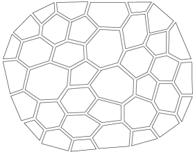
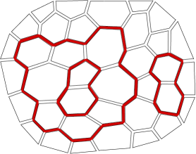
a                                                             b

Figure 1: a)  A trivalent planar graph $\Gamma$ with a boundary    b)  A loop configuration on $\Gamma$ for the ordinary boundary condition. The loops avoid the boundary as they avoid themselves

The Dirichlet boundary condition, was originally defined for the dense phase of the loop gas [20, 21, 22] and requires that an open line starts at each point on the boundary. The dilute version of this boundary condition depends on an adjustable parameter, which controls the number of the open lines. In terms of the $O(n)$ spins the Dirichlet boundary condition is obtained by switching on a constant magnetic field $\vec{B}$ acting on the boundary spins. This modifies the integration measure in (3.1) by a factor

$$\prod_{r\in\partial\Gamma}\Big{(}1+\,\vec{B}\cdot\vec{S}(r)\Big{)}\,,$$ (3.4)

where the product goes over all boundary sites $r$. The loop expansion with this boundary measure contains open lines having both ends at the boundary, each weighted with a factor $\vec{B}^{2}$.

The dilute anisotropic (DJS) boundary condition is defined as follows. The $n$ components of the $O(n)$ spin are split into two sets, ${(1)}$ and ${(2)}$, containing respectively ${n^{{}_{{(1)}}}}$ and ${n^{{}_{(2)}}}$ components, with ${n^{{}_{{(1)}}}}+{n^{{}_{(2)}}}=n$. This leads to a decomposition of the $O(n)$ spin as

$$\vec{S}=\vec{S}_{{}^{(1)}}+\vec{S}_{{}^{(2)}},\quad\vec{S}_{{}^{(1)}}\cdot\vec{S}_{{}^{(2)}}=0.$$ (3.5)

The DJS boundary condition is introduced by an extra factor associated with the boundary links,

$$\prod_{\left\langle\,rr^{\prime}\!\,\right\rangle\in\partial\Gamma}\Big{(}1+\sum_{\alpha=1,2}\lambda_{{}^{(\alpha)}}\,\vec{S}_{{}^{(\alpha)}}(r)\cdot\vec{S}_{{}^{{(\alpha)}}}(r^{\prime})\Big{)}\,.$$ (3.6)

This boundary interaction is invariant under the subgroup of independent rotations of $\vec{S}_{(1)}$ and $\vec{S}_{(2)}$. The boundary term changes the loop expansion. The loops are now allowed to pass along the boundary links as shown in Fig. 2. We have to introduce loops of two colors, ${(1)}$ and ${(2)}$, having fugacities respectively ${n^{{}_{{(1)}}}}$ and ${n^{{}_{(2)}}}$. A loop of color $(\alpha)$ that visits ${\cal N}$ boundary links acquires an additional weight factor $\lambda_{{}^{(\alpha)}}^{\cal N}$. For the loops that do not touch the boundary, the contributions of the two colors sum up to ${n^{{}_{{(1)}}}}+{n^{{}_{(2)}}}=n$ and we obtain the same weight as with the ordinary boundary condition.

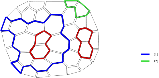
Figure 2: A loop configuration for the JS boundary condition. The loops in the bulk (in red) have fugacity $n$, while the loops that touch the boundary (in blue and green) have fugacities ${n^{{}_{{(1)}}}}$ or ${n^{{}_{(2)}}}$ depending on their color.

3.2 Coupling to 2D discrete gravity

The disk partition function of the $O(n)$ model on a dynamical lattice is defined as the expectation value of (3.1) in the ensemble of all trivalent planar graphs $\Gamma$ with the topology of the disk. The measure depends on two more couplings, $\bar{\mu}$ and $\bar{\mu}_{B}$, called respectively bulk and boundary cosmological constants, associated with the volume $|\Gamma|=\#(\text{cells})$ and the boundary length $|\partial\Gamma|=\#(\text{external lines})$. The partition function of the disk is a function of $\bar{\mu}$ and $\bar{\mu}_{B}$ and is defined by

$$U(T,\bar{\mu},\bar{\mu}_{B})=\sum_{\Gamma\in\{\text{Disk}\}}\frac{1}{|\partial\Gamma|}\ \left({1\over\bar{\mu}}\right)^{{|\Gamma|}}\left({1\over\bar{\mu}_{B}}\right)^{{|\partial\Gamma|}}Z_{{}_{O(n)}}(T;\Gamma).$$ (3.7)

3.3 Two-point functions of the $L$-leg boundary operators

Our aim is to evaluate the boundary two-point function of two $L$-leg operators separating ordinary and anisotropic boundary conditions. The $L$-leg operator $S_{L}$ is obtained by fusing $L$ spins with flavor indices $a_{1},\dots,a_{n}\in\{1,\dots,n\}$. In terms of the loop gas, the operator $S_{L}$ creates $L$ self and mutually avoiding open lines. We would like to exclude configurations where some of the lines contract among themselves. This can be achieved by taking the antisymmetrized product

$$S_{L}\sim\det_{L\times L}S_{a_{i}}(r_{j}),$$ (3.8)

where $r_{1},\dots,r_{L}$ are $L$ consecutive boundary vertices of the planar graph $\Gamma$, and we put the label $L$ instead of writing its dependence on $a_{1},\dots,a_{L}$ explicitly. The two-point function of the operator $S_{L}$ is evaluated as the partition function of the loop gas in presence of $L$ open lines connecting the points $\{r_{i}\}$ and $\{r^{\prime}_{i}\}$. The open lines are self- and mutually avoiding, and are not allowed to intersect the vacuum loops.

Since the DJS boundary condition breaks the $O(n)$ symmetry into $O({n^{{}_{{(1)}}}})\times O({n^{{}_{(2)}}})$, there are two inequivalent correlation functions of the $L$-leg operators with $Ord/DJS\$ boundary conditions. Indeed, the insertion of $S_{a}$ has different effects depending on whether $a$ belongs to the $O({n^{{}_{{(1)}}}})$ or the $O({n^{{}_{(2)}}})$ sectors. In the first case the open line created by $S_{a}$ acquires a factor $\lambda_{{}^{{(1)}}}$ each time it visites a boundary link. In the second case, the factor is $\lambda_{{}^{(2)}}$. Therefore the boundary spin operators (3.8) with $Ord/DJS\$ boundary conditions split into two classes,

$$S_{L}^{(1)} \sim \det[S_{a_{i}}(r_{j})]\,,\quad a_{1},\dots,a_{L}\in{(1)},$$

$$S_{L}^{(2)} \sim \det[S_{a_{i}}(r_{j})]\,,\quad a_{1},\dots,a_{L}\in{(2)}.$$ (3.9)

We denote the corresponding boundary two-point functions respectively by $D_{L}^{(1)}$ and $D_{L}^{(2)}$.

4 Mapping to the $O(n)$ matrix model

The $O(n)$ matrix model [11, 12] generates planar graphs covered by loops in the same way as the one-matrix models considered in the classical paper [29] generate empty planar graphs. The model involves the hermitian $N\times N$ matrices ${\bf M}$ and ${\bf Y}_{a}$, where the flavor index $a$ takes $n$ values. The partition function is given by an $O(n)$-invariant matrix integral

$${\cal Z}_{N}(T)\sim\int d{\bf M}\,d^{n}{\bf Y}\,e^{-\beta\,\text{tr}\left(\frac{1}{2}{\bf M}^{2}+\frac{T}{2}\vec{\bf Y}^{2}-\frac{1}{3}{\bf M}^{3}-{\bf M}\vec{\bf Y}^{2}\right)}.$$ (4.1)

This integral can be considered as the partition function of a zero-dimensional QFT with Feynman rules given in Fig. 3, where we used the ’t Hooft double-line notations. The graphs made of such double-lined propagators are known as fat graphs. The ‘vacuum energy’ of the matrix model represents a sum over connected fat graphs, which can be also considered as discretized two-dimensional surfaces of all possible genera. As the action is quadratic in the matrices ${\bf Y}_{a}$, their propagators arrange in closed loops carrying a flavor $a$. The sum of all Feynman graphs with given connectivity can be viewed as the sum over all configurations of self and mutually avoiding loops on a given discretized surface. The weight of each loop is given by the product of factors $1/T$, one for each link, and the number of flavors $n$. We are interested in the large $N$ limit

$$N\to\infty,\qquad\beta/N=\bar{\mu}^{2}~{}~{}(\text{fixed})\,,$$ (4.2)

in which only fat graphs of genus zero survive [30].

The basic observable in the matrix model is the resolvent

$$W(\bar{\mu}_{B})=\frac{1}{\beta}\left\langle\,\text{tr}{1\over\bar{\mu}_{B}-{\bf M}}\,\right\rangle\,,$$ (4.3)

evaluated in the ensemble (4.1). The resolvent is the one-point function with ordinary boundary conditions and is related to the disk partition function by $W=-\partial_{\bar{\mu}_{B}}U$.

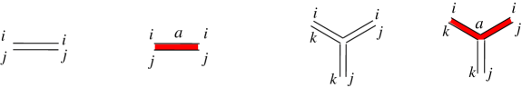
$1/\beta$                      $1/\beta T$                     $\beta$                       $\beta$

Figure 3: Feynman rules for the $O(n)$ matrix model

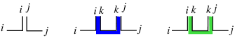
                 $1/\bar{\mu}_{B}$          $\lambda_{{}^{{(1)}}}/\bar{\mu}_{B}^{2}$          $\lambda_{{}^{(2)}}/\bar{\mu}_{B}^{2}$

Figure 4: The constituents of the DJS boundary generated by ${\bf M}$, $\vec{\bf Y}_{(1)}^{2}$ and $\vec{\bf Y}_{(2)}^{2}$: a non-occupied site, a sequence of two sites visited by a loop of color ${(1)}$, and a sequence of two sites visited by a loop of color ${(1)}$

The one-point function with Dirichlet boundary condition is obtained by adding a term $\vec{B}\cdot\vec{\bf Y}$ which expresses the coupling with the magnetic field on the boundary. This leads to a more-complicated resolvent

$$R(\bar{\mu}_{B},\vec{B}^{2})={1\over\beta}\left\langle\,{\rm tr}{1\over\bar{\mu}_{B}-{\bf M}-\vec{B}\cdot\vec{\bf Y}}\,\right\rangle.$$ (4.4)

In order to include the anisotropic boundary conditions in this scheme, we decompose the vector $\vec{\bf Y}$ into a sum of an ${n^{{}_{{(1)}}}}$-component vector $\vec{\bf Y}_{{}^{(1)}}$ and an ${n^{{}_{(2)}}}$-component vector $\vec{\bf Y}_{{}^{(2)}}$ as in (3.5):

$$\vec{\bf Y}=\vec{\bf Y}_{{}^{(1)}}+\vec{\bf Y}_{{}^{(2)}},\quad\vec{\bf Y}_{{}^{(1)}}\cdot\vec{\bf Y}_{{}^{(2)}}=0.$$ (4.5)

The one-point function with ordinary and DJS boundary conditions is given by the resolvent

$$H(\bar{\mu}_{B},\lambda_{{}^{{(1)}}},\lambda_{{}^{(2)}})=\frac{1}{\beta}\left\langle\,\text{tr}{1\over\bar{\mu}_{B}-{\bf M}-{1\over\bar{\mu}_{B}}\sum_{\alpha=1,2}\lambda_{{}^{(\alpha)}}\vec{\bf Y}_{(\alpha)}^{2}}\,\,\right\rangle\,.$$ (4.6)

The two extra terms are the operators creating boundary links containing segments of lines of type ${(1)}$ and ${(2)}$, as shown in Fig.4. Each such operator created two boundary sites, hence the factor $1/\bar{\mu}_{B}$.

The matrix integral measure becomes singular at ${\bf M}=T/2$. We perform a linear change of the variables

$${\bf M}=T\big{(}\tfrac{1}{2}+{\bf X}\big{)}\,,$$ (4.7)

which sends this singular point to ${\bf X}=0$. After a suitable rescaling of $\vec{\bf Y}$ and $\beta$, the matrix model partition function takes the canonical form

$${\cal Z}_{N}\sim\int d{\bf X}\,d^{n}{\bf Y}e^{\beta{\rm tr}[-V({\bf X})+{\bf X}\vec{\bf Y}^{2}]}\,,$$ (4.8)

where $V(x)$ is a cubic potential

$$V(x)=\sum_{j=0}^{3}\frac{g_{j}}{j}x^{j}=-\frac{T}{3}\Big{(}x+\tfrac{1}{2}\Big{)}^{3}+\frac{1}{2}\Big{(}x+\tfrac{1}{2}\Big{)}^{2}.$$ (4.9)

We introduce the spectral parameter $x$ which is related to the lattice boundary cosmological constant $\bar{\mu}_{B}$ by

$$\bar{\mu}_{B}=T\big{(}x+\tfrac{1}{2}\big{)}\,.$$ (4.10)

Now the one-point function with ordinary boundary condition is

$$W(x)=\frac{1}{\beta}\left\langle\text{tr}{\bf W}(x)\right\rangle,$$ (4.11)

where the matrix

$${\bf W}(x)~{}\stackrel{{\scriptstyle\text{def}}}{{=}}~{}\frac{1}{x-{\bf X}}\,.$$ (4.12)

creates a boundary segment with open ends. In the following we will call $x$ boundary cosmological constant. We also redefine the boundary couplings $\lambda_{{}^{(\alpha)}}$ in (4.6) as

$$\lambda_{{}^{(\alpha)}}\to{\lambda_{{}^{(\alpha)}}\,\bar{\mu}_{B}},\quad\alpha=1,2\,.$$ (4.13)

Then the operator that creates a boundary segment with DJS boundary condition is

$${\bf H}(y)~{}\stackrel{{\scriptstyle\text{def}}}{{=}}~{}\frac{1}{y-{\bf X}-\lambda_{{}^{{(1)}}}\vec{\bf Y}_{{}^{(1)}}^{2}-\lambda_{{}^{(2)}}\vec{\bf Y}_{{}^{(2)}}^{2}}\,.$$ (4.14)

The boundary $L$-leg operators are represented by the antisymmetrized products

$${\bf S}_{L}\stackrel{{\scriptstyle\text{def}}}{{=}}{\bf Y}_{a_{1}}{\bf Y}_{a_{2}}\cdots{\bf Y}_{a_{L}}\pm\text{permutations}\,.$$ (4.15)

The boundary two-point function of the $L$-leg operator with $Ord/Ord$ boundary conditions is given by the expectation value

$$D_{L}(x_{1},x_{2})~{}\stackrel{{\scriptstyle\text{def}}}{{=}}~{}\frac{1}{\beta}\left\langle\text{tr}\big{[}{\bf W}(x_{1}){\bf S}_{L}{\bf W}(x_{2}){\bf S}_{L}\big{]}\right\rangle.$$ (4.16)

The role of the operators ${\bf W}(x_{1})$ and ${\bf W}(x_{2})$ is to create the two boundary segments with boundary cosmological constants respectively $x_{1}$ and $x_{2}$. The two insertions ${\bf S}_{L}$ generate $L$ open lines at the points separating the two segments. It is useful to extend this definition to the case $L=0$, assuming that $S_{0}$ is the boundary identity operator. In this simplest case the expectation value (4.16) is evaluated instantly as

$$D_{0}(x_{1},x_{2})~{}=~{}\frac{1}{\beta}\left\langle\text{tr}\big{[}{\bf W}(x_{1}){\bf W}(x_{2})\big{]}\right\rangle~{}=~{}\frac{W(x_{2})-W(x_{1})}{x_{1}-x_{2}}.$$ (4.17)

The two-point functions (4.16) for $L\geq 1$ were computed in [21, 22].

In the case of a DJS boundary condition, the matrix model realization of the two types of boundary $L$-leg operators is given by the antisymmetrized products (4.15), with the restrictions on the components as in (3.3). The boundary two-point functions with $Ord/DJS\$ boundary conditions are evaluated by the expectation values

$$D_{0}(x,y) = \frac{1}{\beta}\Big{\langle}\text{tr}\big{[}{\bf W}(x){\bf H}(y)\big{]}\Big{\rangle}$$ (4.18)

and for $L\geq 1$,

$$D_{L}^{(1)}(x,y) = \frac{1}{\beta}\Big{\langle}\text{tr}\big{[}{\bf W}(x){\bf S}_{L}^{(1)}{\bf H}(y){\bf S}_{L}^{(1)}\big{]}\Big{\rangle},$$ (4.19)

$$D_{L}^{(2)}(x,y) = \frac{1}{\beta}\Big{\langle}\text{tr}\big{[}{\bf W}(x){\bf S}_{L}^{(2)}{\bf H}(y){\bf S}_{L}^{(2)}\big{]}\Big{\rangle}.$$ (4.20)

Apart of the DJS boundary parameter ${n^{{}_{{(1)}}}}$ and the boundary couplings $\lambda_{{}^{{(1)}}},\lambda_{{}^{(2)}}$ for the second segment, they depend on the boundary cosmological constants $x$ and $y$ associated with the two segments of the boundary.

5 Loop equations

Our goal is to evaluate the two-point functions (4.19) in the continuum limit, when the area and the boundary length of the disk are very large. They will be obtained as solution of a set of Ward identities, called loop equations, which follow from the translational invariance of the integration measure in (4.1), and in which the ${n^{{}_{{(1)}}}}$ enters as a parameter. The solutions of the loop equations are analytic functions of ${n^{{}_{{(1)}}}}$ which can take any real value. We will restrict our analysis to the ‘physical’ case $0\leq{n^{{}_{{(1)}}}}\leq n$, when the correlation functions have good statistical limit. Here we summarize the loop equations which will be extensively studied in following sections. The proofs are given in Appendix A.

5.1 Loop equation for the resolvent

The loop equation for the resolvent is known [31], but we nevertheless recall it here in order to set up a self-contained description of the method. The resolvent $W(x)$ splits into a singular part $w(x)$ and a polynomial $W_{\rm reg}(x)$:

$$W(x)\stackrel{{\scriptstyle\text{def}}}{{=}}W_{\rm reg}(x)+w(x)\,.$$ (5.1)

The regular part is given by

$$W_{\rm reg}(x) = \frac{2V^{\prime}(x)-nV^{\prime}(-x)}{4-n^{2}}=-a_{0}-a_{1}x-a_{2}x^{2}\,,$$

$$a_{0} = -{g_{1}\over 2+n}=\frac{T-2}{4(2+n)},$$

$$\quad a_{1} = -{g_{2}\over 2-n}=\frac{T-1}{2-n},$$

$$\quad a_{2} = -{g_{3}\over 2+n}=\frac{T}{2+n}.$$ (5.2)

The function $w(x)$ satisfies a quadratic identity

$$w^{2}(x)+w^{2}(-x)+nw(x)w(-x)=A+Bx^{2}+Cx^{4}\,.$$ (5.3)

The coefficients $A,B,C$ as functions of $T$, $\bar{\mu}$ and $W_{1}=\langle\text{tr}X\rangle$ can be evaluated by substituting the large-$x$ asymptotics

$$w(x)=-W_{\rm reg}(x)+\frac{\bar{\mu}^{-2}}{x}+\frac{\langle\text{tr}X\rangle}{\beta x^{2}}+O(x^{-3})$$ (5.4)

in (5.3). The solution of the loop equation (5.3) with the asymptotics (5.4) is given by a meromorphic function with a single cut $[a,b]$ on the first sheet, with $a<b<0$. This equation can be solved by an elliptic parametrization and the solution is expressed in terms of Jacobi theta functions [32].

5.2 Loop equations for the boundary two-point functions with Ord/DJS boundary conditions

The two-point correlators (4.16) with ordinary boundary conditions are known to satisfy the integral recurrence equations [21, 22]

$$D_{L+1}=W\star D_{L}\,.$$ (5.5)

The “$\star$-product” is defined for any pair of meromorphic functions, analytic in the right half plane $\text{Re}(x)\geq 0$ and vanishing at infinity,

$$[f\star g](x)~{}\stackrel{{\scriptstyle\text{def}}}{{=}}~{}-\oint\limits_{{\cal C}_{-}}\frac{dx^{\prime}}{2\pi i}\frac{f(x)-f(x^{\prime})}{x-x^{\prime}}g(-x^{\prime}),$$ (5.6)

with the contour ${\cal C}_{-}$ encircling the left half plane $\text{Re}x<0$. These equations actually hold for a more general set of two-point correlators, which have ordinary boundary condition on one segment and an arbitrary boundary condition on the other segment [13]. Thus the boundary two-point functions (4.19) and (4.20) for $L\geq 1$ satisfy the same recurrence equations

$$D_{L+1}^{(1)} = W\star D_{L}^{(1)}\,,$$

$$D_{L+1}^{(2)} = W\star D_{L}^{(2)}\,.$$ (5.7)

Using the recurrence relation, the correlation functions of the $L$-leg operators can be obtained recursively from those of the one-leg operators $D_{1}^{(1)}$ and $D_{1}^{(2)}$.

The correlator $D_{0}$, defined by (4.18), and the correlators $D_{1}^{(1)}$ and $D_{1}^{(2)}$, which we normalize as

$$D_{1}^{(\alpha)}(x,y) = \frac{1}{\beta n^{{}_{(\alpha)}}}\sum_{a}\left\langle\text{tr}\big{[}{\bf W}(x){\bf Y}^{(\alpha)}_{a}{\bf H}(y){\bf Y}^{(\alpha)}_{a}\big{]}\right\rangle\qquad(\alpha=1,2),$$ (5.8)

can be determined by the following pair of bilinear functional equations, derived in Appendix A. In order to shorten the expressions, here and below we use the shorthand notation

$$\overline{F(x)}\stackrel{{\scriptstyle\text{def}}}{{=}}F(-x)\,.$$ (5.9)

The two equations then read

$$W-H+D_{0}(x-y)+\sum_{\alpha=1,2}n^{{}_{(\alpha)}}\lambda_{{}^{(\alpha)}}\left((\lambda_{{}^{(\alpha)}}D_{0}-1)\overline{D_{1}^{(\alpha)}}+\overline{W}\,D_{0}\right) = 0\,,$$ (5.10)

$$P+D_{0}\left(H-V^{\prime}+W+n\overline{W}\right)+\sum_{\alpha=1,2}n^{{}_{(\alpha)}}\left(\lambda_{{}^{(\alpha)}}D_{0}-1\right)\overline{D_{1}^{(\alpha)}} = 0\,.$$ (5.11)

The second equation involves an unknown linear function of $x$:

$$P(x,y) \stackrel{{\scriptstyle\text{def}}}{{=}} \frac{1}{\beta}\left\langle\text{tr}\frac{V^{\prime}(x)-V^{\prime}({\bf X})}{x-{\bf X}}{\bf H}(y)\right\rangle=g_{2}H(y)+g_{3}H_{1}(y)+xg_{3}H(y).$$ (5.12)

Equations (5.10) and (5.11) can be solved in favor of $D_{1}^{(1)}$ or $D_{1}^{(2)}$. If we define

$${\cal A}^{(1)} \stackrel{{\scriptstyle\text{def}}}{{=}} \lambda_{{}^{{(1)}}}D_{0}-1,$$

$${\cal B}^{(1)} \stackrel{{\scriptstyle\text{def}}}{{=}} (\lambda_{{}^{{(1)}}}-\lambda_{{}^{(2)}}){n^{{}_{{(1)}}}}\{\lambda_{{}^{{(1)}}}D_{1}^{(1)}+W\}-\lambda_{{}^{(2)}}\left(\overline{W}-\overline{V^{\prime}}+H\right)-x-y,$$ (5.13)

$${\cal C}^{(1)} \stackrel{{\scriptstyle\text{def}}}{{=}} \lambda_{{}^{{(1)}}}\lambda_{{}^{(2)}}P+(\lambda_{{}^{{(1)}}}+\lambda_{{}^{(2)}})H-x+y-(\lambda_{{}^{{(1)}}}-\lambda_{{}^{(2)}})\left(W+{n^{{}_{{(1)}}}}\overline{W}\right)-\lambda_{{}^{(2)}}V^{\prime}\,,$$

and similarly for ${\cal A}^{(2)},{\cal B}^{(2)},{\cal C}^{(2)}$, with an obvious exchange ${(1)}\leftrightarrow{(2)}$, then (5.10) and (5.11) take the following factorized form:

$${\cal A}^{(\alpha)}\overline{{\cal B}^{(\alpha)}}~{}=~{}{\cal C}^{(\alpha)}\qquad(\alpha=1,2)\,.$$ (5.14)

Equations (5.14) are the main instrument of our analysis of the DJS boundary conditions.

It is convenient to define the functions $D_{0}^{(\alpha)}$ by

$$D_{0}^{(\alpha)}\stackrel{{\scriptstyle\text{def}}}{{=}}\frac{D_{0}}{1-\lambda_{{}^{(\alpha)}}D_{0}}\qquad(\alpha=1,2)\,.$$ (5.15)

In Appendix A we show that with this definition the recurrence equations (5.7) hold also for $L=0$. The equation for $L=0$ is a consequence of (5.14).

5.3 Loop equation for the two-point function with Ord/Dir boundary conditions

On the flat lattice, the DJS boundary condition with ${n^{{}_{{(1)}}}}=1$ is equivalent, for a special choice of the boundary parameters, to the Dirichlet boundary condition defined by the boundary factor (3.4). In order to make the comparison on the dynamical lattice, we will formulate and solve the loop equation for the two-point function of the BCC operator with ordinary/Dirichlet boundary conditions.

Assume that the magnetic field points at the direction $a=1$. Then the correlator in question is given in the matrix model by the expectation value

$$\Omega(x,y)={1\over\beta}\left\langle\,{\rm tr}{\bf W}(x){\bf R}(y)\,\right\rangle,\qquad{\bf R}(y)={1\over y-{\bf X}-B{\bf Y}_{1}}\,.$$ (5.16)

To obtain the loop equation we start with the identity

$$W(x)-R(y)=(y-x)\Omega(x,y)-B\Omega_{1}(x,y),$$ (5.17)

where we denoted by $R(y)$ the one-point function with Dirichlet boundary condition,

$$R(x)={1\over\beta}\left\langle\,{\rm tr}{\bf R}(y)\,\right\rangle,$$ (5.18)

and introduced the auxiliary function

$$\Omega_{1}(x,y)={1\over\beta}\left\langle\,{\rm tr}{{\bf Y_{1}}\bf W}(x){\bf R}(y)\,\right\rangle.$$ (5.19)

The function $\Omega_{1}$ satisfies the identity

$$\Omega_{1}(x,y)=B\,\oint_{{\cal C}_{-}}{dx_{1}\over 2\pi i}\ {\Omega(x_{1},y)\Omega(-x_{1},y)\over x-x_{1}}\,,$$ (5.20)

which follows from (A.3). After symmetryzing with respect to $x$ we get

$$\Omega_{1}(x,y)+\Omega_{1}(-x,y)=B\,\Omega(x,y)\Omega(-x,y).$$ (5.21)

From here we obtain a quadratic functional equation for the correlator $\Omega$:

$$(x-y)\Omega(x,y)-(x+y)\Omega(-x,y)+W(x)+W(-x)+B^{2}\,\Omega(x,y)\Omega(-x,y)=2R(y).$$ (5.22)

The linear term can be eliminated by a shift

$$G(x,y)=B\,\Omega(x,y)-{x+y\over B}\,.$$ (5.23)

The function $G$ satisfies

$$G(x,y)G(-x,y)=-W(x)-W(-x)+2R(y)-{x^{2}-y^{2}\over B^{2}}\,.$$ (5.24)

This equation is to be compared with the loop equation (5.14) for Ord/DJS boundary conditions, with ${n^{{}_{{(1)}}}}=1$ and $\lambda_{{}^{(2)}}=0$:

$${1\over\lambda_{{}^{{(1)}}}}{\cal A}^{(1)}(x,y){\cal B}^{(1)}(-x,y)~{}=~{}-W(x)-W(-x)+H(y)-{x-y\over\lambda_{{}^{{(1)}}}}\,.$$ (5.25)

These two equations coincide in the limit $B,\lambda_{{}^{{(1)}}}\to\infty$. To see this it is sufficient to notice that in the limit $\lambda_{{}^{{(1)}}}\to\infty$ we have the relation ${\cal B}^{(1)}=y{\cal A}^{(1)}$. The exact relation between ${\cal A}^{(1)}$ (with ${n^{{}_{{(1)}}}}=1,\lambda_{{}^{(2)}}=0$) and $G$ in this limit follows from the definitions of $D_{0}$ and $\Omega$:

$${\cal A}^{(1)}(x,y^{\prime})=B{G(x,y)-G(x,-y)\over 2y},\quad\lambda_{{}^{{(1)}}}=B^{2},\quad y^{\prime}=y^{2}\qquad(B\to\infty).$$ (5.26)

6 Scaling limit

In this section we will study the continuum limit of the solution, in which the sum over lattices is dominated by those with diverging area and boundary length. The continuum limit is achieved when the couplings $x$, $y$ and $\bar{\mu}$ are tuned close to their critical values.

Once the bulk coupling constants are set to their critical values, we will look for the critical line in the space of the boundary couplings $y,\lambda_{{}^{{(1)}}}$ and $\lambda_{{}^{(2)}}$. After the shift (4.7) the bondary cosmological constant $x$ has its critical value at $x=0$, while the critical value of $y$ in general depends on the values of $\lambda_{{}^{{(1)}}}$ and $\lambda_{{}^{(2)}}$.

6.1 Scaling limit of the disk one-point function

Here we recall the derivation of the continuum limit of the one-point function $W(x)$ from the functional equation (5.3). Even if the result is well known, we find useful to explain how it is obtained in order to set up the logic of our approach to the solution of the functional equations (5.14).

In the limit $x\to 0$, the boundary length $|\partial\Gamma|$ of the planar graphs in (3.7) becomes critical. The quadratic functional equation (5.3) becomes singular at $x\to 0$ when the coefficient $A$ on the r.h.s. vanishes. This determines the critical value of the cosmological constant $\bar{\mu}$, for which the volume $|\Gamma|$ of a typical planar graph diverges. The condition that the coefficient $B$ of the linear term vanishes determines the critical value of the temperature coupling $T=T_{c}$ for which the length of the loops diverges:

$$T_{c}=1+\sqrt{\tfrac{2-n}{6+n}}\in[1,2]\,.$$ (6.1)

Near the critical temperature the coefficient $B$ is proportional to $T-T_{c}$.

We rescale $x\to\epsilon x$, where $\epsilon$ is a small cutoff parameter with dimension of length, and define the renormalized coupling constants as

$$\bar{\mu}-\bar{\mu}_{c}\sim\epsilon^{2}\mu\,,\quad T-T_{c}\sim\epsilon^{2\theta}t\,$$ (6.2)

and write (5.1) as

$$W(x)\stackrel{{\scriptstyle\text{def}}}{{=}}W_{\rm reg}+\epsilon^{1+\theta}w(x)\,.$$ (6.3)

The renormalized bulk and boundary cosmological constants are coupled respectively to the renormalized area $A$ and boundary length $\ell$ of the graph $\Gamma$ defined as

$$A=\epsilon^{2}\,|\Gamma|,\qquad\ell=\epsilon\,|\partial\Gamma|\,.$$ (6.4)

In the following we define the dimensions of the scaling observables by the way they scale with $x$. We will say that the quantity $f$ has dimension $d$ if the ratio $f/x^{d}$ is invariant with respect to rescalings. In this case we write $[f]=d$. The continuous quantities introduced until now have scaling dimensions

$$[x]=1,\ [\mu]=2,\ [t]=2\theta,\ [w]=1+\theta\,.$$ (6.5)

The scaling resolvent $w(x)$ is a function with a cut on the negative axis in the $x$-plane. It can be obtained from the general solution found in [32] by taking the limit in which the cut extends to the semi-infinite interval $[-\infty,-M]$. To determine $M$ as a function of $\mu$ and $t$ one has to solve a system of difficult transcendental equations. A simpler indirect method was given in [33]. We begin by noticing that the term $Cx^{4}$ in (5.3) drops out because it vanishes faster than the other terms when $x\to 0$, and $B=B_{1}\,t$, where $B_{1}$ depends only on $n$. Introducing a hyperbolic map which resolves the branch point at $x=-M$,

$$x=M\cosh\tau\,,$$ (6.6)

we obtain a quadratic functional equation for the entire function $w(\tau)\equiv w[x(\tau)]$:

$$w^{2}(\tau+i\pi)+w^{2}(\tau)+n\,w(\tau+i\pi)w(\tau)=A+B_{1}tM^{2}\cosh^{2}\tau\,.$$ (6.7)

This equation does not depend on the cutoff $\epsilon$, which justifies the definition of the renormalized thermal coupling in (6.2). Then the unique solution of this equation is, up a factor which depends on the normalization of $t$,

$$w(\tau)=M^{1+\theta}\cosh(1+\theta)\tau+tM^{1-\theta}\cosh(1-\theta)\tau\,.$$ (6.8)

One finds $B_{1}=4\sin^{2}(\pi\theta)$ and $A=\sin^{2}(\pi\theta)(M^{1+\theta}-tM^{1-\theta})^{2}$ for this solution.

The function $M=M(\mu,t)$ can be evaluated using the fact that the derivative $\partial_{\mu}W(x)$ depends on $\mu$ and $t$ only through $M$. As a consequence, in the derivative of the solution in $\mu$ at fixed $x$,

$$\partial_{\mu}w=-M\partial_{\mu}M\left((1+\theta)M^{\theta}-(1-\theta)tM^{-\theta}\right)\frac{\sinh\theta\tau}{\sinh\tau},$$ (6.9)

the factor in front of the hyperbolic function must be proportional to $M^{\theta-1}$:

$$\partial_{\mu}M\Big{(}(1+\theta)M^{\theta}-(1-\theta)tM^{-\theta}\Big{)}\sim M^{\theta-1}.$$

Integrating with respect to $\mu$ one finds, for certain normalization of $\mu$,

$$\mu=(1+\theta)M^{2}-tM^{2-2\theta}.$$ (6.10)

To summarize, the disk bulk and the boundary one-point functions with ordinary boundary condition, $-\partial_{\mu}U$ and $-\partial_{x}U$, are given in the continuum limit in the following parametric form:

$$-\partial_{x}U|_{\mu} = {M^{1+\theta}}{\cosh((1+\theta)\tau)}\ +t\,{M^{1-\theta}}{\cosh(1-\theta)\tau},$$ (6.11)

$$-\partial_{\mu}U|_{x} \sim \ \,\,\,M^{\theta}\,\cosh\,\theta\tau,$$

$$x\ \ \ = \ \ \ M\,\cosh\tau,$$

with the function $M(\mu,t)$ determined from the transcendental equation (6.10). The expression for $\partial_{\mu}U$ was obtained by integrating (6.9).

The function $M(t,\mu)$ plays an important role in the solution. Its physical meaning can be revealed by taking the limit $x\to\infty$ of the bulk one-point function $-\partial_{\mu}U(x)$. Since $x$ is coupled to the length of the boundary, in the limit of large $x$ the boundary shrinks and the result is the partition function of the $O(n)$ field on a sphere with two punctures, the susceptibility $u(\mu,t)$. Expanding at $x\to\infty$ we find

$$-\partial_{\mu}U\sim x^{\theta}-M^{2\theta}\,x^{-\theta}+\text{ lower powers of }x$$ (6.12)

(the numerical coefficients are omitted). We conclude that the string susceptibility is given, up to a normalization, by

$$u=M^{2\theta}.$$ (6.13)

The normalization of $u$ can be absorbed in the definition of the string coupling constant $g_{s}\sim 1/\beta$. Thus the transcendental equation (6.10) for $M$ gives the equation of state of the loop gas on the sphere,

$$(1+\theta)\,u^{1\over\theta}-\,t\,u^{1-\theta\over\theta}=\mu\,\,.$$ (6.14)

The equation of state (6.14) has three singular points at which the three-point function of the identity operator $\partial_{\mu}u$ diverges. The three points correspond to the critical phases of the loop gas on the sphere. At the critical point $t=0$ the susceptibility scales as $u\sim\mu^{\theta}$. This is the dilute phase of the loop gas, in which the loops are critical, but occupy an insignificant part of the lattice volume. The dense phase is reached when $t/x^{\theta}\to-\infty$. In the dense phase the loops remain critical but occupy almost all the lattice and the susceptibility has different scaling, $u\sim\mu^{1-\theta\over\theta}$. The scaling of the susceptibility in the dilute and in the dense phases match with the values (2.4) and (2.6) of the central charge of the corresponding matter CFTs. Considered on the interval $-\infty<t<0$, the equation of state (6.14) describes the massless thermal flow [34] relating the dilute and the dense phases.

At the third critical point $\partial_{\mu}M$ becomes singular but $M$ itself remains finite. It is given by

$$t_{c}=\frac{1+\theta}{1-\theta}\,M_{c}^{2\theta}\ >0,\qquad\mu_{c}=-\theta\frac{1+\theta}{1-\theta}\,M_{c}^{2}\ <0.$$ (6.15)

Around this critical point $\mu-\mu_{c}\sim(M-M_{c})^{2}+\cdots$, hence the scaling of the susceptibility is that of pure gravity, $u\sim(\mu-\mu_{c})^{1/2}$.

6.2 The phase diagram for the DJS boundary condition

We found the scaling limit of the one-point function (4.11) as a function of the renormalized bulk couplings, $\mu$ and $t$, and the coupling $x$ characterizing the ordinary boundary. Now, analyzing the loop equation (5.14) for the two-point functions, we will look for the possible scaling limits for the couplings $y$, $\lambda_{{}^{{(1)}}}$ and $\lambda_{{}^{(2)}}$, characterizing the DJS boundary.

As in the previous subsection, we will write down the conditions that the regular parts of the source terms ${\cal C}^{(\alpha)}$ vanish. Let us introduce the isotropic coupling $\lambda$ and the anisotropic coupling $\Delta$ as

$$\lambda_{{}^{{(1)}}}=\lambda+{\textstyle{1\over 2}}\Delta,\ \lambda_{{}^{(2)}}=\lambda-{\textstyle{1\over 2}}\Delta\,$$ (6.16)

and substitute (5.1) in the r.h.s. of (5.14). We obtain

$${\cal C}^{(1)} = c_{0}+c_{1}x+c_{2}x^{2}-\,\Delta(w+{n^{{}_{{(1)}}}}\overline{w})\,,$$

$${\cal C}^{(2)} = c_{0}+c_{1}x+c_{2}x^{2}+\,\Delta(w+{n^{{}_{(2)}}}\overline{w})\,,$$ (6.17)

where the coefficients $c_{0}$ and $c_{1}$ are functions of $\lambda$ and $\Delta$:

$$c_{0} = (\lambda^{2}-{{\textstyle{1\over 4}}}\Delta^{2})(g_{2}H+g_{3}H_{1})+2\lambda H+y-\lambda g_{1}-\Delta\,{g_{1}({n^{{}_{{(1)}}}}-{n^{{}_{(2)}}})\over 2(2+n)}$$ (6.18)

$$c_{1} = (\lambda^{2}-{{\textstyle{1\over 4}}}\Delta^{2})g_{3}H-1-\lambda g_{2}+\Delta\,{g_{2}({n^{{}_{{(1)}}}}-{n^{{}_{(2)}}})\over 2(2-n)}.$$ (6.19)

$$c_{2} = -g_{3}\left(\lambda+{{n^{{}_{{(1)}}}}-{n^{{}_{(2)}}}\over 2(2+n)}\Delta\right).$$ (6.20)

For generic values of the couplings $y,\lambda$ and $\Delta$, the coefficient $c_{0}$ is non-vanishing. The condition $c_{0}=0$ determines the critical value $y_{c}$ where the length of the DJS boundary diverges. Once the boundary cosmological constant is tuned to its critical value, the condition $c_{1}=0$ determines the critical lines in the space of the couplings $\lambda_{{}^{{(1)}}}$ and $\lambda_{{}^{(2)}}$, where the DJS boundary condition becomes conformal. The two equations

$$c_{0}(y,\lambda,\Delta)=0,\qquad c_{1}(y,\lambda,\Delta)=0\qquad(\mu=t=0)$$ (6.21)

define a one-dimensional critical submanifold in the space of the boundary couplings $\{y,m,\Delta\}$:

$$\lambda=\lambda^{*}(\Delta)\,.$$ (6.22)

Obviously ${\cal A}^{(1)}$ and ${\cal A}^{(2)}$ cannot be simultaneously zero. Therefore the curve (6.22) consists of two branches, which correspond to different conformal DJS boundary conditions, the lines of anisotropic special transitions $AS_{(1)}$ and $AS_{(2)}$:

$$AS_{(1)}: \quad{\cal A}^{(1)}=0,\ {\cal A}^{(2)}\neq 0;$$

$$AS_{(2)}: \quad{\cal A}^{(2)}=0,\ {\cal A}^{(1)}\neq 0.$$ (6.23)

The branch $AS_{(1)}$ corresponds to $\Delta>0$, while the branch $AS_{(2)}$ corresponds to $\Delta<0$. Consider the behavior of correlators $D_{0}^{(\alpha)}$ on the two branches of the critical line. By the definition (5.15), the two correlators $D_{0}^{(1)}$ and $D^{(2)}_{0}$ are related by

$$D_{0}^{(1)}=\dfrac{D_{0}^{(2)}}{1-\Delta D_{0}^{(2)}},\quad D_{0}^{(2)}=\dfrac{D_{0}^{(1)}}{1+\Delta D_{0}^{(1)}}.$$ (6.24)

On the branch $AS_{(1)}$ the correlator $D^{(1)}_{0}$ diverges while $D^{(2)}_{0}$ remines finite, and vice versa. Assume that $\lambda_{{}^{{(1)}}}$ and $\lambda_{{}^{(2)}}$ are positive. Then $D^{(\alpha)}_{0}$ are both positive by construction. If $\Delta=\lambda_{{}^{{(1)}}}-\lambda_{{}^{(2)}}>0$, then the coefficients of the geometric series

$${D_{0}^{(1)}}=\sum_{k=0}^{\infty}{\Delta^{k}\left(D_{0}^{{(2)}}\right)^{k+1}}$$ (6.25)

are all positive and $D^{(1)}_{0}$ diverges, while $D^{(2)}_{0}\to 1/\Delta$. Thus the branch $AS_{(1)}$, where $D_{0}^{(1)}$ diverges, is associated with $\Delta>0$. On this branch the probability that the loops of color ${(1)}$ touch the DJS boundary is critically enhanced. In the correlator $D_{0}^{(1)}$, the ordinary boundary behaves as a loop of type ${(1)}$ and can touch the DJS boundary. The geometrical progression (6.25) reflects the possibility of any number of such events, each contributing a factor $\Delta$. Conversely, the ordinary boundary for the correlator $D^{(2)}_{0}$ behaves as a loop of type ${(2)}$, since such loops almost never touch the DJS boundary. On the branch $AS_{(2)}$ the situation is reversed.

It is not possible to solve explicitly the conditions of criticality (6.21) without extra information, because they contain two unknown functions of the three couplings, $H$ and $H_{1}$. Nevertheless, the qualitative picture can be reconstructed.

First let us notice that the form of the critical curve can be evaluated in the particular cases ${n^{{}_{{(1)}}}}=n$ and ${n^{{}_{{(1)}}}}=0$. In the first case ${n^{{}_{(2)}}}=0$ and the correlation functions do not depend on $\lambda_{{}^{(2)}}$ and so the coefficients $c_{1}$ and $c_{2}$ depend on $\lambda$ and $\Delta$ through the combination $\lambda_{{}^{{(1)}}}=\lambda+\Delta/2$. Similarly one considers the case ${n^{{}_{{(1)}}}}=0$. The phase diagram in these two cases represents an infinite straight line separating the ordinary and the extraordinary transitions:

$$\lambda^{*}(\Delta)=\begin{cases}\lambda_{c}-\Delta/2&\text{ if }{n^{{}_{{(1)}}}}=n,\\ \lambda_{c}+\Delta/2&\text{if }{n^{{}_{{(1)}}}}=0.\end{cases}$$ (6.26)

The critical line crosses the axis $\Delta=0$ at the special point $\lambda=\lambda_{c}$. The value of $\lambda_{c}$ can be evaluated by solving (6.21) for ${n^{{}_{{(1)}}}}=n$ and $\lambda_{{}^{(2)}}=0$. The result is

$$\lambda_{c}={\sqrt{(6+n)(2-n)}\over 1-n}.$$ (6.27)

For general ${n^{{}_{{(1)}}}}\in[0,n]$ we can determine three points of the critical curve:

$$\{\lambda_{{}^{{(1)}}},\lambda_{{}^{(2)}}\}=\{{1-n\over 1-{n^{{}_{{(1)}}}}}\lambda_{c},\ 0\},\quad\{0,\ {1-n\over 1-{n^{{}_{(2)}}}}\lambda_{c}\},\quad\{\lambda_{c},\lambda_{c}\}\,.$$ (6.28)

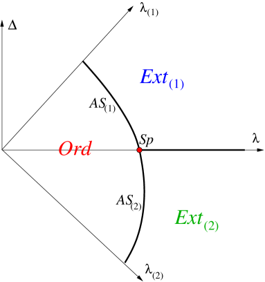
Figure 5: Phase diagram in the rotated $({\lambda_{{}^{{(1)}}}},{\lambda_{{}^{(2)}}})$ plane for $n<1$ and ${n^{{}_{{(1)}}}}>{n^{{}_{(2)}}}$. The ordinary and the extraordinary phases are separated by a line of anisotropic special transitions, which consists of two branches, $AS_{(1)}$ and $AS_{(2)}$. The two extraordinary phases, $Ext_{(1)}$ and $Ext_{(2)}$, are separated by the isotropic line $\Delta=0$

In the two limiting cases considered above the critical line, given by equation (6.26), crosses the anisotropic line without forming a cusp. Is this the case in general? Let us consider the vicinity of the special point $(\lambda,\Delta)=(\lambda_{c},0)$. In the vicinity of the special point a new scaling behavior occurs. In this regime the term $x^{2}$ in (6.17) cannot be neglected. The requirement that all terms in (6.17) have the same dimension determines the scaling of the anisotropic coupling $\Delta$:

$$[\Delta]=1-\theta.$$ (6.29)

In order to determine the form of the critical curve near the special point, we return to the equations (6.21) and consider the behavior near the special point of the unknown functions $H(y)={1\over\beta}\left\langle\,{\rm tr}{\bf H}(y)\,\right\rangle$ and $H_{1}(y)={1\over\beta}\left\langle\,{\rm tr}{\bf X}{\bf H}(y)\,\right\rangle$, which depend implicitly on $\lambda$ and $\Delta$. For $t=\mu=0$, these functions can be decomposed, just as the one-point function with ordinary boundary condition, $W(x)$, into regular and a singular parts:

$$H(y)=H^{\rm reg}(y)+h(y),\quad H_{1}(y)=H_{1}^{\rm reg}(y)+\text{cst}\cdot h(y)\,.$$ (6.30)

On the critical curve $\lambda=\lambda^{*}(\Delta)$ the singular part of $H$ vanishes and the coefficient $c_{1}$ given by eq. (6.19) can be Taylor expanded in $\lambda-\lambda_{c}$ and $\Delta$:

$$c_{1}(m,\Delta)\equiv A_{1}\,(\lambda-\lambda_{c})+B_{1}\,({n^{{}_{{(1)}}}}-{n^{{}_{(2)}}})\Delta+A_{2}\,(\lambda-\lambda_{c})^{2}+B_{2}\,\Delta^{2}+\dots=0.$$ (6.31)

If $A_{1}\neq 0$, the critical curve is given by a regular function of $\lambda$ and $\Delta$, the critical curve is a continuous line which crosses the real axis at $\lambda=\lambda_{c}$ without forming a cusp. This form of the curve differs from the predictions of [2] and [3], where a cusp-like form is predicted by a scaling argument. We will see later that the fact that the critical curve is analytic at the special point does not contradict the scaling (6.29).

6.3 Scaling limit of the functional equation for the disk two-point function

6.3.1 The scaling limit for $\Delta\neq 0$

Consider first the case when the anisotropic coupling $\Delta$ is finite and assume that we are on the branch $AS_{(1)}$ where $\Delta>0$. Then the $x^{2}$ term on the r.h.s. can be neglected, because it is subdominant compared to $w\sim x^{1+\theta}$. The scaling limit corresponds to the vicinity of the critical submanifold where the two coefficients $c_{0}$ and $c_{1}$ scale respectively as $x^{1+\theta}$ and $x^{\theta}$.

We are now going to find the scaling limit of the loop equations (5.14). In the scaling limit we can retain only the singular parts of the correlators $D_{L}^{{(1)},{(2)}}$, which we denote by $d_{L}^{{(1)},{(2)}}$ ($L=0,1,...$). We define the functions $d_{0}^{(1)}$ and $d_{0}^{(2)}$ by

$$D_{0}^{(1)}=\,d_{0}^{(1)},\quad D_{0}^{(2)}={1\over\Delta-\,d_{0}^{(2)}}\approx{1\over\Delta}+{1\over\Delta^{2}}\,d_{0}^{(2)}.$$ (6.32)

Then the relation (6.24) implies

$$d_{0}^{{(1)}}\,d_{0}^{{(2)}}=-1.$$ (6.33)

We define in general $d_{L}^{{(1)},{(2)}}$ as the singular part of $D_{L}^{{(1)},{(2)}}$, with the normalization chosen so that the recurrence equation (5.7) holds for any $L\geq 0$:

$$d^{(1)}_{L+1} = w\star d^{(1)}_{L}\,,$$

$$d^{(2)}_{L+1} = w\star d^{(2)}_{L}.$$ (6.34)

On the branch $AS_{(1)}$ the first of the two equations (5.14) becomes singular, since ${\cal A}^{(1)}$ vanishes while ${\cal A}^{(2)}$ remains finite. We write this equation in terms of $d_{0}^{(2)}$ and $d_{1}^{(1)}$ using that

$${\cal A}^{{(1)}}=\lambda_{{}^{{(1)}}}\,d_{0}^{(2)},\quad{\cal B}^{{(1)}}={\Delta\over\lambda_{{}^{{(1)}}}}\,d_{1}^{{(1)}}.$$ (6.35)

We get

$$\hskip 85.35826pt{d^{(2)}_{0}}\,\overline{d^{(1)}_{1}}+w+{n^{{}_{{(1)}}}}\overline{w}=\mu_{B}-t_{B}x\,\,,\hskip 85.35826pt(\Delta>0)$$ (6.36)

where $\mu_{B}$ and $t_{B}$ are defined by

$${c_{0}\over\Delta}=\mu_{B},\qquad{c_{1}\over\Delta}=-t_{B}\,.$$ (6.37)

Once the solution of (6.37) is known, all two-point functions $d_{L}^{(\alpha)}$ can be computed by using the recurrence equations (6.3.1).

The scaling limit near the branch $AS_{(2)}$ ($\Delta<0$) is obtained by using the symmetry ${n^{{}_{{(1)}}}}\leftrightarrow{n^{{}_{(2)}}},\ \Delta\leftrightarrow-\Delta$. In this case one obtains another equation

$$\hskip 85.35826pt{d^{(1)}_{0}}\,\overline{d^{(2)}_{1}}+w+{n^{{}_{(2)}}}\overline{w}=\mu_{B}-t_{B}x\,\,.\hskip 85.35826pt(\Delta<0)$$ (6.38)

Note that the relation (6.33) is true on both branches of the critical line.

The map $\{y,\lambda\}\to\{\mu_{B},t_{B}\}$ defined by (6.18), (6.19) and (6.37) represents a coordinate change in the space of couplings which diagonalizes the scaling transformation. The coupling $\mu_{B}$ is the renormalized boundary cosmological constant for the DJS boundary. The coupling $t_{B}$ is the renormalized boundary matter coupling, which defines the DJS boundary condition. The dimensions of these couplings are

$$[\mu_{B}]=1+\theta,\qquad[t_{B}]=\theta.$$ (6.39)

Once we choose $y$ so that $\mu_{B}=0$, the condition $t_{B}=0$ gives the critical curve where the anisotropic special transitions take place. If the function $t_{B}$ is regular near the critical line $\lambda=\lambda^{*}(\Delta)$, then it can be replaced by the linear approximation

$$t_{B}\sim\lambda^{*}(\Delta)-\lambda.$$ (6.40)

The deformations in the directions $t_{B}$ and $\Delta$, are driven by some Liouville dressed boundary operators ${\mathcal{O}}_{t_{B}}^{B}$ and ${\mathcal{O}}_{\Delta}^{B}$. Knowing the dimensions of $t_{B}$ and $\Delta$, we can determine the Kac labels of these operators with the help of the KPZ formula. The general rule for evaluating the Kac labels in 2D gravity with matter central charge (2.4) is the following. If a coupling constant has dimension $\alpha$, then the corresponding operator has Kac labels $(r,s)$ determined by

$$\alpha=\alpha_{r,s}=\text{min}\left(1+{\theta\over 2}\pm{(1+\theta)r-s\over 2}\right).$$ (6.41)

The details of the identification are given in Appendix B. We find

$${\mathcal{O}}_{t_{B}}^{B}={\cal O}_{1,3}^{B},\qquad{\mathcal{O}}_{\Delta}^{B}={\cal O}_{3,3}^{B}.$$ (6.42)

Near the special point we have

$$\Delta\sim t_{B}^{1/\phi},\qquad\phi={\theta\over 1-\theta}={\alpha_{1,3}\over\alpha_{3,3}}<1.$$ (6.43)

Since $t_{B}$ and $\lambda$ scale differently, there is no contradiction between the scaling (6.43) and the analyticity of the critical curve near the special point.

6.3.2 The scaling limit in the isotropic direction $(\Delta=0)$

Along the isotropic line $\Delta=0$ the two functional equations (5.14) degenerate into a single equation for the correlator $D_{0}$:

$${\cal A}\equiv\lambda D_{0}-1=-{y-x+\lambda(2H+\lambda P-V^{\prime})\over y-x+\lambda\left(W+H-V^{\prime}\right)}.$$ (6.44)

In order to evaluate $D_{1}=D_{1}^{(1)}=D_{1}^{(2)}$, we can consider the linear order in $\Delta$. It is however easier to use the fact that $D_{0}$ and $D_{1}$ do not depend on the splitting $n={n^{{}_{{(1)}}}}+{n^{{}_{(2)}}}$. Furthermore, if we choose ${n^{{}_{{(1)}}}}=n$ and $\lambda_{{}^{{(1)}}}=\lambda$, the observables do not depend on $\lambda_{{}^{(2)}}$, which can be chosen to be zero. Taking ${n^{{}_{{(1)}}}}=n$, $\lambda_{{}^{{(1)}}}=m$ and ${n^{{}_{(2)}}}=\lambda_{{}^{(2)}}=0$, we obtain from (5.14)

$$\overline{{\cal B}^{{(1)}}}\big{|}_{{n^{{}_{{(1)}}}}=n}\equiv\lambda\left(\lambda\overline{D_{1}}+n\overline{W}\right)+x-y={y-x+\lambda(H-W-n\overline{W})\over\lambda D_{0}-1}\,.$$ (6.45)

From these expressions it is clear how the scaling of the singular parts of $D_{0}$ and $D_{1}$, which we denote respectively by $d_{0}$ and $d_{1}$, change when we go from $\lambda=0$ to $\lambda=\lambda_{c}$. When $\lambda=0$ we have $H(y)=W(y)$ and $D_{0}$ is the disk partition function with ordinary boundary conditions and two marked points on it, eq. (4.17). When $\lambda=\lambda_{c}$ and $y=y_{c}$,

$$d_{0}=g_{3}{x^{2}\over w}\sim x^{1-\theta},\qquad d_{1}={w(w+n\bar{w})\over g_{3}\ x^{2}}\sim x^{2\theta}\qquad(\lambda=\lambda_{c},\ y=y_{c}).$$ (6.46)

6.3.3 Dirichlet versus DJS 

Now we will focus on the special case ${n^{{}_{{(1)}}}}=1$ and compare the scaling behavior with that for the Dirichlet boundary conditions. The critical behavior of the two-point correlator in both cases is the same, but the boundary coupling constants correspond to different boundary operators.

Consider the functional equation (5.25) for the correlator with Ord/DJS boundary conditions when ${n^{{}_{{(1)}}}}=1$. The critical value of $\lambda_{{}^{{(1)}}}$ is infinite in this case, see equation (6.28). The scaling limit of (5.25) is

$$d_{0}^{(1)}(x,y)d_{1}^{(2)}(-x,y)~{}=~{}-w(x)-w(-x)+\mu_{B}-{x\over\lambda_{{}^{{(1)}}}}\,.$$ (6.47)

The last term remains finite if $\lambda_{{}^{{(1)}}}$ tends to infinity as $x^{-\theta}$. The scaling boundary coupling can be identified as $t_{B}=1/\lambda_{{}^{{(1)}}}$ and equation (6.47) takes the general form (6.36). What is remarkable here is that the boundary temperature constant need not to be tuned. Equation (6.47) holds for any value of $\lambda_{{}^{{(1)}}}$. On the other hand, when $t_{B}=1/\lambda_{{}^{{(1)}}}$ is small, the last term describes the perturbation of the $AS_{(1)}$ boundary condition by the thermal operator ${\mathcal{O}}_{1,3}$ with $\alpha_{1,3}=\theta$. When $\lambda_{{}^{{(1)}}}$ is small, the last term accounts for the perturbation of the ordinary boundary condition by the two-leg boundary operator ${\mathcal{O}}_{3,1}$ with $\alpha_{3,1}=-\theta$, whose matter component is an is irrelevant operator.

Now let us take the scaling limit of the quadratic functional equation (5.24) for the correlator with Ord/Dir boundary conditions. At $x=0$ the equation (5.24) becomes algebraic. The critical value $y=y_{c}$, where the solution develops a square root singularity, is determined by

$$2W(0)-2R(y_{c})+{y_{c}^{2}/B^{2}}=0.$$

We can write equation (5.24) as

$$G(x,y)G(-x,y)=\mu_{B}-w(x)-w(-x)-{x^{2}\over B^{2}}\,,$$ (6.48)

where

$$\mu_{B}=2w(0)+2[R(y)-R(y_{c})]+{y^{2}-y_{c}^{2}\over B^{2}}.$$ (6.49)

For any finite value of $B$, the scaling limit of this equation is

$$G(x,y)G(-x,y)=\mu_{B}-w(x)-w(-x)\,.$$ (6.50)

The $x^{2}$ term survives only if $B$ vanishes as $x^{1-\theta\over 2}$:

$$[B]=(1-\theta)/2=\alpha_{2,1}.$$ (6.51)

This is the expected answer, because ${\mathcal{O}}_{2,1}^{B}$ is the one-leg boundary operator which creates an open line starting at the boundary. We conclude that the Dirichlet and the DJS boundary conditions have the same scaling limit, but in the first case the boundary coupling $\lambda$ corresponds to a relevant perturbation and it is sufficient give it any finite value, while in the second case the boundary coupling $\lambda_{{}^{{(1)}}}$ corresponds to an irrelevant perturbation and therefore must be infinitely strong.

7 Spectrum of the boundary operators

Let us denote by $\alpha^{(1)}_{L}$ and $\alpha^{(2)}_{L}$ the scaling dimensions respectively of $d^{(1)}_{L}$ and $d^{(2)}_{L}$:

$$\alpha^{(\alpha)}_{L}=[d^{(\alpha)}_{L}]\qquad(L\geq 0,\ a=1,2).$$ (7.1)

The recurrence equations (6.3.1) tell us that the dimensions grow linearly with $L$:

$$\alpha_{L}^{(\alpha)}=L[w]+\alpha_{0}^{(\alpha)}\,.$$ (7.2)

These relations make sense in the dilute phase, where $[w]=1+\theta$, as well as in the dense phase, where $[w]=1-\theta$. In addition, by (6.33) we have

$$\alpha_{0}^{(1)}+\alpha_{0}^{(2)}=0.$$ (7.3)

Thus all scaling dimensions are expressed in terms of $\alpha_{0}^{(1)}$.

Let us evaluate $\alpha_{0}$ for the branch $AS_{(1)}$ of the critical line. We thus assume that $\Delta$ is finite and positive sufficiently far from the isotropic special point. Take $\mu=\mu_{B}=t_{B}=0$ and write the shift equations which follow from (6.36),

$$AS_{(1)}:\qquad{d^{(1)}_{0}(e^{i\pi}x)\over d^{(1)}_{0}(e^{-i\pi}x)}={w(e^{-i\pi}x)+{n^{{}_{{(1)}}}}w(x)\over w(e^{i\pi}x)+{n^{{}_{{(1)}}}}w(x)}.$$ (7.4)

The one-point function (6.8) behaves as $w\sim x^{1+\theta}$ in the dilute phase ($t=0$) and as $w\sim x^{1-\theta}$ in the dense phase ($t\to-\infty$). In both cases the r.h.s. is just a phase factor. Since all the couplings except for $x$ have been turned off, $d_{0}^{(1)}(x)$ should be a simple power function of $x$. Substituting $d_{L}^{(1)}(x)\sim x^{\alpha_{L}^{(1)}}$ in (7.4), we find

$${n^{{}_{{(1)}}}}={\sin\pi(\alpha_{0}^{(1)}\pm\theta)\over\sin\pi\alpha_{0}^{(1)}}\,,\qquad\left(+\ \text{for dilute},\ -\ \text{for dense}\right)\,.$$ (7.5)

This equation determines the exponent $\alpha^{(1)}_{0}$ up to an integer. In the parametrization (2.15) we have $\alpha_{0}^{(1)}=-\theta r+j_{\text{dil}}$ in the dilute phase and $\alpha_{0}^{(1)}=\theta r+j_{\text{den}}$ in the dense phase.

The integers $j_{\text{dil}}$ and $j_{\text{den}}$ can be fixed by additional restrictions on the exponents. Let us assume that $\lambda_{{}^{{(1)}}}$ and $\lambda_{{}^{(2)}}$ are non-negative, $n\geq 0$ and the boundary parameter $r$ is in the ‘physical’ interval $1\leq r\leq 1/\theta-1$, where both ${n^{{}_{{(1)}}}}$ and ${n^{{}_{(2)}}}$ are non-negative. These assumptions guarantee that the Boltzmann weights are positive and the loop expansion of the observables has good statistical meaning. Since all loop configurations that enter in the loop expansion of the one-point function $W(x)$ are present in the loop expansions of ${\cal A}^{{(\alpha)}}$ and ${\cal B}^{{(\alpha)}}$, the singularity of these observables when $\lambda\to\lambda^{*}(\Delta)$ must not be weaker than that of $W$. In other words, the scaling dimensions of $d_{0}^{(2)}\sim{\cal A}^{{(1)}}$ and $d_{1}^{(1)}\sim{\cal B}^{{(1)}}$ must not be larger than the scaling dimension of the one-point function $w$:

$$\alpha_{0}^{(2)}<[w],\quad\alpha_{1}^{(1)}<[w].$$ (7.6)

Since $\alpha_{0}^{(2)}+\alpha_{1}^{(1)}=[w]$, this also means that $\alpha_{0}^{(2)}$ and $\alpha_{1}^{(1)}$ are non-negative. Taking into account that $[w]=1\pm\theta$ in the dilute/dense phase, we get the bound

$$-(1\pm\theta)\leq\alpha^{{(1)}}_{0}\leq 0\qquad\left(+\ \text{for dilute},\ -\ \text{for dense}\right).$$ (7.7)

This bound determines $j_{\text{dil}}=0$ and $j_{\text{den}}=-1$. As a consequence, on the branch $AS_{(1)}$ of the critical line the dimensions $\alpha^{(1)}_{L}=[d^{(1)}_{L}]$ in the dilute and in the dense phases are given by

$$AS_{(1)}:\quad\begin{array}[]{lll}\alpha^{(1)}_{L}=L(1+\theta)-\theta r,&\alpha_{L}^{(2)}=L(1+\theta)+\theta r&\qquad\text{(dilute phase)}\\ \alpha^{(1)}_{L}=L(1-\theta)+\theta r-1,&\alpha_{L}^{(2)}=L(1-\theta)-\theta r+1&\qquad\text{(dense phase)}.\end{array}$$ (7.8)

Note that the results for the dense phase are valid not only in the vicinity of the critical line $AS_{(1)}$, but in the whole half-plane $\Delta>0$.

By the symmetry ${(1)}\leftrightarrow{(2)}$, the exponents $\alpha^{(1)}_{L}$ on the branch $AS_{(1)}$ and the exponents $\alpha^{(2)}_{L}$ on the branch $AS_{(2)}$ should be related by ${n^{{}_{{(1)}}}}\leftrightarrow{n^{{}_{(2)}}}$, or equivalently $r\leftrightarrow 1/\theta-r$:

$$AS_{(2)}:\quad\begin{array}[]{lll}\alpha^{(1)}_{L}=L(1+\theta)-\theta r+1,&\alpha^{(2)}_{L}=L(1+\theta)+\theta r-1,&\qquad\text{(dilute phase)}\\ \alpha^{(1)}_{L}=L(1-\theta)+\theta r,&\alpha^{(2)}_{L}=L(1-\theta)-\theta r&\qquad\text{(dense phase)}.\end{array}$$ (7.9)

The scaling exponents of the two-point functions of the $O(n)$ model coupled to 2D gravity allow, through the KPZ formula [23, 24], to determine the conformal weights of the matter boundary operators. In the dilute phase, where the Kac parametrization is given by (2.5), the correspondence between the scaling dimension $\alpha$ of a boundary two-point correlator and the conformal weight $h_{r,s}$ of the corresponding matter boundary field is given by

$$\alpha=(1+\theta)r-s\quad\to\quad h=h_{r,s}\,\qquad\text{(dilute phase).}\$$ (7.10)

In the dense phase, where the Kac labels are defined by (2.7), one obtains, taking into account that the identity boundary operator for the ordinary boundary condition has ‘wrong’ dressing,

$$\alpha=r-s(1-\theta)\quad\to\quad h=h_{r,s}\,\qquad\text{(dense phase)}.$$ (7.11)

From (7.10) and (7.11) we determine the scaling dimensions of the $L$-leg boundary operators (3.3):

$$AS_{(1)}:\quad\begin{array}[]{lll}S_{L}^{(1)}\to{\mathcal{O}}^{B}_{r-L,r},&S_{L}^{(2)}\to{\mathcal{O}}^{B}_{r+L,r}&\text{(dilute phase)}\\ S_{L}^{(1)}\to{\mathcal{O}}^{B}_{r-1,r-L},&S_{L}^{(2)}\to{\mathcal{O}}^{B}_{r-1,r+L}&\text{(dense phase)}.\end{array}$$ (7.12)

$$AS_{(2)}:\qquad\begin{array}[]{lll}S_{L}^{(1)}\to{\mathcal{O}}^{B}_{r-L,r+1},&S_{L}^{(2)}\to{\mathcal{O}}^{B}_{r+L,r+1}&\qquad\text{(dilute phase)}\\ S_{L}^{(1)}\to{\mathcal{O}}^{B}_{r,r-L},&S_{L}^{(2)}\to{\mathcal{O}}^{B}_{r,r+L}&\qquad\text{(dense phase)}.\end{array}$$ (7.13)

These conformal weights are in accord with the results of [7], [13], [14], [3]. We remind that the scaling dimensions are determined up to a symmetry of the Kac parametrization:

$$h_{r,s}=h_{-r,-s},\quad h_{r,s-1}=h_{r+1/\theta,s+1/\theta}\qquad\text{(dilute phase)}$$ (7.14)

$$h_{r,s}=h_{-r,-s},\quad h_{r+1,s}=h_{r+1/\theta,s+1/\theta}\qquad\text{(dense phase)}.$$ (7.15)

Comparing the scaling dimensions in the dilute and in the dense phase, we see that the bulk thermal flow $t\,{\mathcal{O}}_{1,3}$ transforms the boundary operator ${\mathcal{O}}_{r,s}$ in the dilute phase into the boundary operator ${\mathcal{O}}_{s-1,r}$ in the dense phase. For the rational points $\theta=1/p$, our results for the endpoints of the bulk thermal flow driven by the operator $t\,{\mathcal{O}}_{1,3}$ match the perturbative calculations performed recently in [15].

In the $O(n)$ model the boundary parameter $r$ is continuous and we can explore the limit $r\to 1$, in which the BCC operator ${\mathcal{O}}_{r,r}$ carries the same Kac labels as the identity operator. Let us call this operator $\tilde{\mathcal{O}}_{1,1}^{B}$. The bulk thermal flow transforms the operators $\tilde{\mathcal{O}}_{1,1}^{B}$ and ${\mathcal{O}}_{1,1}^{B}$ into two different boundary operators in the dense phase. Hence there are at least two distinct boundary operators with Kac labels $(1,1)$: the identity operator and the limit $r\to 1$ of the operator ${\mathcal{O}}_{r,r}^{B}$.

8 Solution of the loop equations in the scaling limit

We are going to study two particular cases where the analytic solution of the functional equations (6.36) and (6.38) is accessible. First we will evaluate the two-point function on the two branches $AS_{(1)}$ and $AS_{(2)}$ of the critical line, where the $O(n)$ field is conformal invariant both in the bulk and on the boundary. In this case $t=t_{B}=0$ and the boundary two-point function is that of Liouville gravity. The three couplings are introduced by the world sheet action of Liouville gravity with matter central charge (2.4), which we write symbolically as

$${\cal S}_{\text{Liouv}}={\cal S}_{\text{free}}+\int\limits_{\text{bulk}}\mu\,{\mathcal{O}}_{1,1}+\hskip-17.07182pt\int\limits_{\text{Ord. boundary}}\hskip-17.07182ptx\,{\mathcal{O}}_{1,1}^{B}+\hskip-14.22636pt\int\limits_{\text{DJS\ boundary}}\hskip-14.22636pt\mu_{B}\,{\mathcal{O}}_{1,1}^{B}.$$ (8.1)

Since the perturbing operators in this case are Liouville primary fields,

$${\mathcal{O}}_{1,1}\sim e^{2b\phi},\quad{\mathcal{O}}_{1,1}^{B}\sim e^{b\phi},$$

the two-point function is given by the product of matter and Liouville two-point functions. Up to a numerical factor, the solution as a function of $\mu$ and $\mu_{B}$ must be given by the boundary two-point function in Liouville theory [35]. We will see that indeed the functional equation (6.36) is identical to a functional equation obtained in [35] using the operator product expansion in boundary Liouville theory.

In the second case we are able to solve, we take $\mu=\mu_{B}=0$ and non-zero matter couplings $t$ and $t_{B}$. This case is more interesting, because it is not described by the standard Liouville gravity. The corresponding world sheet action is symbollically written as

$${\cal S}={\cal S}_{\text{free}}+\int\limits_{\text{bulk}}t\,{\mathcal{O}}_{1,3}+\hskip-17.07182pt\int\limits_{\text{Ord. boundary}}\hskip-14.22636ptx\,{\mathcal{O}}_{1,1}^{B}+\hskip-17.07182pt\int\limits_{\text{DJS\ boundary}}\hskip-14.22636ptt_{B}\,{\mathcal{O}}_{1,3}^{B}.$$ (8.2)

The worldsheet theory described by this action is more complicated than Liouville gravity, because it does not enjoy the factorization properties of the latter. The boundary two-point correlator does not factorize, for finite $t$ and/or $t_{B}$, into a product of matter and Liouville correlators, as is the case for the action (8.1). This is because the perturbing operators ${\mathcal{O}}_{1,3}$ and ${\mathcal{O}}_{1,3}^{B}$ have both matter and Liouville components:

$${\mathcal{O}}_{1,3}\sim\Phi_{1,3}\,e^{2b(1-\theta)\phi},\quad{\mathcal{O}}_{1,3}^{B}\sim\Phi_{1,3}^{B}\,e^{b(1-\theta)\phi}.$$

Let us mention that the theory of random surfaces described by the action (8.2) has no obvious direct microscopic realization. Our solution interpolates between the two-point functions for the dilute ($t=0$) and the dense ($t\to-\infty$) phases of the loop gas, on one hand, and between the anisotropic special $(t_{B}=0)$ and ordinary/extraordinary boundary conditions ($t_{B}\to\pm\infty$), on the other hand.

8.1 Solution for $t=0,t_{B}=0$

In the dilute phase ($t=0$) the solution (6.6) - (6.8) for the boundary one-point function takes the form

$$x=M\cosh\tau,\quad w(x)=M^{1+\theta}\cosh(1+\theta)\tau.$$ (8.3)

Then the loop equations (6.36) become a shift equation

$$d^{(2)}_{0}(\tau)\,d^{(1)}_{1}(\tau\pm i\pi)+w_{0}\cosh\left[(1+\theta)\tau\pm i\pi(1-r)\theta\right]=\mu_{B}-t_{B}M\cosh\tau\,,$$ (8.4)

where we introduced the constant

$$w_{0}=M^{1+\theta}{\sin\pi\theta\over\sin\pi r\theta}.$$ (8.5)

At the point $t_{B}=0$, where the DJS boundary condition is conformal, this equation can be solved explicitly. After a shift $\tau\to\tau\mp i\pi$ we write it, using (6.33), as

$$\,d^{(1)}_{1}(\tau)=\left[w_{0}\cosh\left[(1+\theta)\tau\pm i\pi r\theta\right]-\mu_{B}\,\right]\ d^{(1)}_{0}(\tau\pm i\pi).$$ (8.6)

If we parametrize $\mu_{B}$ in terms of a new variable $\sigma$ as

$$\mu_{B}~{}=~{}w_{0}\cosh(1+\theta)\sigma,$$ (8.7)

the loop equation turns out to be identical to the functional identity for the boundary Liouville two-point function [35], which we recall in Appendix B. In the Liouville gravity framework, $\tau$ and $\sigma$ parametrize the FZZT branes corresponding to the ordinary and anisotropic special boundary conditions.

The loop equations for the dense phase ($t\to-\infty$), are given by (8.6) with $\theta$ sign-flipped. This equation describes the only scaling limit in the dense phase. The term with $t_{B}$ is absent in the dense phase, because it has dimension $1+\theta$, while the other terms have dimension $1-\theta$. In this case, the loop equation gets identical to the functional identity for the Liouville boundary two-point function if we parametrize $\mu_{B}$ as

$$\mu_{B}~{}=~{}w_{0}\cosh\big{(}1-\theta)\sigma.$$ (8.8)

8.2 Solution for $\mu=0,\ \mu_{B}=0$

Here we solve the loop equation (6.36) in the scaling limit with $\mu=\mu_{B}=0$ but keeping $x$, $t$ and $t_{B}$ finite. Let us first find the expression for the one-point function $w(x)$ for $\mu=0$. The equation (6.10) has in this case two solutions, $M=0$ and $M=(1+\theta)^{-1}t^{1\over 2\theta}$. One can see [33] that the first solution is valid for $t<0$, while the second one is valid for $t>0$. Therefore when $\mu=0$ and $t\leq 0$, the solution (6.6)-(6.8) takes the following simple form:

$$w(x)=x^{1+\theta}+tx^{1-\theta}\qquad(t\leq 0).$$ (8.9)

Introduce the following exponential parametrization of $x,t,t_{B}$ in terms of $\tau,\gamma,\tilde{\gamma}$:

$$x=e^{\tau},\quad t=-e^{2\gamma\theta},\quad t_{B}=-2w_{0}\,e^{\gamma\theta}\sinh(\tilde{\gamma}\theta),\quad w_{0}=\frac{\sin(\pi\theta)}{\sin(\pi r\theta)}.$$ (8.10)

In terms of the new variables, equation (6.36) with $\mu_{B}=\mu=0$ acquires the form

$${d^{(1)}_{1}(\tau)/d^{(1)}_{0}(\tau\pm i\pi)} = w_{0}\left(-2e^{\gamma\theta}\sinh(\tilde{\gamma}\theta)e^{\tau}+e^{(1+\theta)\tau\pm i\pi r\theta}-e^{2\theta\gamma}e^{(1+\theta)\tau\pm i\pi r\theta}\right)\,$$ (8.11)

$$= 4w_{0}\,e^{\tau+\gamma\theta}\cosh\frac{\theta(\tau-\gamma+\tilde{\gamma}\pm i\pi r)}{2}\sinh\frac{\theta(\tau-\gamma-\tilde{\gamma}\pm i\pi r)}{2}\,.\qquad$$

Taking the logarithm of both sides we obtain a linear difference equation, which can be solved explicitly. The solution is given by

$$AS_{(1)}:\quad\begin{array}[]{lll}d_{0}^{(1)}(\tau)&=&{1\over w_{0}}e^{-\frac{\tau}{2}-\gamma(r\theta-\frac{1}{2})+\frac{\tilde{\gamma}}{2}}V_{-r}(\tau-\gamma+\tilde{\gamma})V_{\frac{1}{\theta}-r}(\tau-\gamma-\tilde{\gamma}),\\ d_{1}^{(1)}(\tau)&=&-e^{\frac{\tau}{2}+\gamma(\frac{1}{2}+\theta-r\theta)+\frac{\tilde{\gamma}}{2}}V_{1-r}(\tau-\gamma+\tilde{\gamma})V_{1+\frac{1}{\theta}-r}(\tau-\gamma-\tilde{\gamma}),\end{array}$$ (8.12)

where the function $V_{r}(\tau)$ is defined by

$$\log V_{r}(\tau)~{}\stackrel{{\scriptstyle\text{def}}}{{=}}~{}-\frac{1}{2}\int\frac{d\omega}{\omega}\left[\frac{e^{-i\omega\tau}\sinh(\pi r\omega)}{\sinh(\pi\omega)\sinh\frac{\pi\omega}{\theta}}-\frac{r\theta}{\pi\omega}\right]\,.\quad$$ (8.13)

The properties of the function $V_{r}(\tau)$ are listed in Appendix C.

The solution (8.12) reproduces correctly the scaling exponents (7.8) and it is unique, assuming that the correlators $d_{0}^{(1)}$ and $d_{1}^{(1)}$ have no poles as functions of $x$. Near the branch $AS_{(2)}$, the functions $d_{0}^{(2)}$ and $d_{1}^{(2)}$ are given by the same expressions (8.12), but with $r$ replaced by $1/\theta-r$.

8.3 Analysis of the solution

To explore the scaling regimes of the solution (8.12) we use the expansion (C) and return to the original variables,

$$e^{\tau}=x,\quad e^{\gamma\theta}=(-t)^{1\over\theta},\quad e^{(\gamma\pm\tilde{\gamma})\theta}=\left(\mp{{t_{B}\over 2}+\sqrt{{t_{B}^{2}\over 4}-t}}\right)^{1\over\theta}.$$ (8.14)

Let us define the function $\hat{V}(x)$ by $V_{r}(\tau)=\hat{V}_{r}(e^{\tau})$. The large $x$ expansion of $\hat{V}_{r}$ goes, according to (C.5), as

$$\hat{V}_{r}(x)=x^{r\theta/2}\left(1+{\sin\pi r\over\sin\pi/\theta}\ x^{-1}+{\sin\pi r\theta\over\sin\pi\theta}\ x^{-\theta}+\dots\right).$$ (8.15)

The expansion at small $x$ follows from the symmetry $\hat{V}(x)=\hat{V}(1/x)$. Written in terms of the original variables, the scaling solution near the branch $AS_{(1)}$ takes the form

$$d_{0}^{(1)}(x) = {1\over w_{0}}\ {(-t)^{-{r\over 2}}\over\sqrt{x}}\ \left(-{t_{B}/2}+\sqrt{{t_{B}^{2}/4}-t}\right)^{{1\over 2\theta}}$$ (8.16)

$$\times \hat{V}_{-r}\left[x\,\left({t_{B}/2}+\sqrt{{t_{B}^{2}/4}-t}\right)^{-{1\over\theta}}\right]\hat{V}_{{1\over\theta}-r}\left[x\left(-{t_{B}/2}+\sqrt{{t_{B}^{2}/4}-t}\right)^{-{1\over\theta}}\right]$$

$$d_{1}^{(1)}(x) = -\sqrt{x}\,t^{1-r\over 2}\left(-{t_{B}/2}+\sqrt{{t_{B}^{2}/4}-t}\right)^{{1\over 2\theta}}$$ (8.17)

$$\times \!\!\hat{V}_{1-r}\!\!\left[x\,\left({t_{B}/2}+\sqrt{{t_{B}^{2}/4}-t}\right)^{-{1\over\theta}}\right]\hat{V}_{1+{1\over\theta}-r}\!\!\left[x\left(-{t_{B}/2}+\sqrt{{t_{B}^{2}/4}-t}\right)^{-{1\over\theta}}\right].\quad$$

The critical regimes of this solution are associated with the limits $t\to-0,-\infty$ and $t_{B}\to 0,\pm\infty$ of the bulk and the boundary temperature couplings.

(i) Dilute phase, anisotropic special transitions

This critical regime is achieved when both $t$ and $t_{B}$ are small. Using the asymptotics (8.15), we find that in the limit $(t_{B}\to 0,t\to-0)$ the expressions (8.16)-(8.17) reproduce the correct scaling exponents (7.8) in the dilute phase:

$$AS_{(1)}:\qquad d_{0}^{(1)}\sim x^{-r\theta},\qquad d_{1}^{(1)}\sim x^{1+\theta-\theta r}\qquad\qquad(t_{B}=0,\ t\to-0).$$ (8.18)

The regime $AS_{(2)}$ is obtained by replacing ${(1)}\to{(2)},\ r\to{1\over\theta}-r$.

(ii) Dilute phase, ordinary transition

At $t\to-0$, the leading behavior of $d_{0}^{(2)}=1/d_{0}^{(1)}$ and $d_{1}^{(1)}$ for large $t_{B}$ is (we omitted all numerical coefficients)

$$\begin{array}[]{lll}d_{0}^{(2)}&\sim&{t_{B}}^{r}\left(1+{t_{B}}^{-\frac{1}{\theta}}x+t_{B}^{-1}\,x^{\theta}+\dots\right)\\ d_{1}^{(1)}&\sim&{t_{B}}^{1-r}\left(x+{t_{B}}^{-\frac{1}{\theta}}x^{2}+t_{B}^{-1}\,x^{\theta+1}+t_{B}^{-2}\,x^{2\theta+1}+\dots\right)\end{array}\quad(t\to-0,\ t_{B}\to+\infty).$$ (8.19)

In the expansion for $d_{0}^{(2)}$, the first singular term, $x^{\theta}$, is the singular part of $D_{0}$ with ordinary/ordinary boundary conditions. In the expansion for $d_{1}^{(1)}$, the first singular term, $x^{1+\theta}$, is the one-point function $w$, while the next term, $x^{2\theta+1}$, is the singular part of the boundary two-point function $D_{1}^{(1)}$ with ordinary/ordinary boundary conditions.

(iii) Dilute phase, extraordinary transition

Now we write the asymptotics of (8.16)-(8.17) in the opposite limit, $t\to-0$, and $t_{B}\to-\infty$:

$$\begin{array}[]{lll}d_{0}^{(2)}&\sim&{t_{B}}^{-{1\over\theta}+r}\left(x+{t_{B}}^{-\frac{1}{\theta}}x^{2}+t_{B}^{-1}\,x^{\theta+1}+t_{B}^{-2}\,x^{2\theta+1}+\dots\right)\\ d_{1}^{(1)}&\sim&{t_{B}}^{{1\over\theta}+1-r}\left(1+{t_{B}}^{-\frac{1}{\theta}}\,x\,+\,t_{B}^{-1}\,x^{\theta}+\dots\right)\end{array}\qquad(t=0,\ t_{B}\to-\infty).$$ (8.20)

This asymptotics reflects the symmetry of the solution (8.12) which maps

$$r\to 1+1/\theta-r,\qquad d_{0}^{(2)}\leftrightarrow d_{1}^{(1)}$$ (8.21)

which is also a symmetry of the loop equations (5.14). In the limit of large and negative $t_{B}$, the function $d_{0}^{(2)}$ behaves as the singular part of the correlator $D_{1}^{(1)}$ with ordinary/ordinary boundary conditions, while $d_{1}^{(1)}$ behaves as the singular part of the correlator $D_{0}$ with ordinary/ordinary boundary conditions.

The asymptotics of the solution at $t_{B}\to\pm\infty$ confirms the qualitative picture proposed in [3] and explained in the Introduction. When $t_{B}$ is large and positive, the loops avoid the boundary and we have the ordinary boundary condition. In the opposite limit, $t_{B}\to-\infty$, the DJS boundary tends to be coated by loop(s). Therefore the typical loop configurations for $D_{1}^{(1)}$ in the limit $t_{B}\to-\infty$ will look like those of $D_{0}^{(1)}$ in the ordinary phase, because the open line connecting the two boundary-changing points will be adsorbed by the DJS boundary. Conversely, the typical loop configurations for $D_{0}^{(1)}$ will look like those of $D_{1}^{(1)}$ in the ordinary phase, because free part of the loop that wraps the DJS boundary will behave as an open line connecting the two boundary-changing points.

We saw that the solution reproduces the qualitative phase diagram for the dilute phase, shown in Fig. 5. Now let us try to reconstruct the phase diagram in the dense phase.

(iv) Dense phase, anisotropic special transitions

For any finite value of $t_{B}$, the dense phase is obtained in the limit $t\to-\infty$. The asymptotics of (8.16)-(8.17) in this limit does not depend on $t_{B}$:

$$d_{0}^{(1)}\sim x^{r\theta-1}\,(-t)^{{1\over 2\theta}-r},\ \quad d_{1}^{(1)}\sim x^{-(1-r)\theta}\ (-t)^{1-r+{1\over 2\theta}}\qquad(t\to-\infty).$$ (8.22)

This means that in the dense phase the DJS boundary condition is automatically conformal for any value of $t_{B}$. The boundary critical behavior does not change with the isotropic boundary coupling $t_{B}$, but it can depend on the anisotropic coupling $\Delta$. The solution (8.16)-(8.17) holds for any positive value of $\Delta$. For negative $\Delta$ we have another solution, which is obtained by replacing ${(1)}\to{(2)}$ and $r\to 1/\theta-r$. Thus in the dense phase there are two possible critical regimes for the DJS boundary, one for positive $\Delta$ and the other for negative $\Delta$, which are analogous to the two anisotropic special transitions in the dilute phase. The domains of the two regimes are separated by the isotropic line $\Delta=0$.

The above is true when $t_{B}$ is finite. If $t_{B}$ tends to $\pm\infty$, we can obtain critical regimes with the properties of the ordinary and the extraordinary transitions.

(v) Dense phase, ordinary and extraordinary transitions

If we expand the solution (8.16)-(8.17) for $-t\gg x^{2\theta}$ and $t_{B}\gg-tx^{-\theta}$, the singular parts of the two correlators will be the same as the correlators with ordinary boundary condition on both sides. For example, instead of the term $t_{B}^{-1}x^{\theta}$ in the expression for $d_{0}^{(2)}$, we will obtain $t^{-1}t_{B}x^{-\theta}$. This is the singular part of the correlator $D_{0}$ with ordinary boundary conditions in the dense phase. Further, the asymptotics of the solution in the limit $-t\gg x^{2\theta}$ and $t_{B}\ll tx^{-\theta}$ is determined by the symmetry (8.21). This critical regime has the properties of the extraordinary transition, in complete analogy with the dilute case. We conclude that the ordinary and the extraordinary transitions exist also in the dense phase, but they are pushed to $t_{B}\to\pm\infty$.

Finally, let us comment on the possible origin of the square-root singularity of the solution (8.16)-(8.17) at $t_{B}^{2}=4t$. This singularity appears in the disordered phase, $t>0$, which is outside the domain of validity of the solution. Nevertheless, one can speculate that this singularity is related to the surface transition, which separates the phases with ordered and disordered spins near the DJS boundary. The singularity in our solution has two branches, $t_{B}=\pm 2\sqrt{t}$, while in the true solution for $t>0$ the negative branch should disappear.

9 Conclusions

In this paper we studied the dilute boundary $O(n)$ model with a class of anisotropic boundary conditions, using the methods of 2D quantum gravity. The loop gas formulation of the anisotropic boundary conditions, proposed by Dubail, Jacobsen and Saleur (DJS ), involves two kinds of loops having fugacities ${n^{{}_{{(1)}}}}$ and ${n^{{}_{(2)}}}=n-{n^{{}_{{(1)}}}}$. Besides the bulk temperature, which controls the length of the loops, the model involves two boundary coupling constants, which define the interaction of the two kinds of loops with the boundary.

The regime where the DJS boundary condition becomes conformal invariant is named in [3] anisotropic special transition. The enhanced symmetry of the model after coupling to gravity system allowed us to solve the model analytically away from the anisotropic special transition. We used the solution to explore the deformations away from criticality which are generated by the bulk and boundary thermal operators.

Our main results can be summarized as follows.

1) We found the phase diagram for the boundary transitions in the dilute phase of the $O(n)$ model with anisotropic boundary interaction. The phase diagram is qualitatively the same as the one obtained in [3] and sketched in the Introduction. The critical line consists of two branches placed above and below the isotropic line. Near the special point the critical curve is given by the same equation on both sides of the isotropic line, which means that the two branches of the critical line meet at the special point without forming a cusp. We also demonstrated that the analytic shape of the critical curve does not contradict the scaling of the two boundary coupling constants. This contradicts the picture drawn in [2] on the basis of scaling arguments, which seems to be supported by the numerical analysis of [3]. Of course we do not exclude the possibility that the origin of the discrepancy is in the fluctuations of the metric.

2) From the singular behavior of the boundary two-point functions we obtained the spectrum of conformal dimensions of the $L$-leg boundary operators between ordinary and anisotropic special boundary conditions, which is in agreement with [3]. In order to establish the critical exponents we used substantially the assumption that ${n^{{}_{{(1)}}}}$ and ${n^{{}_{(2)}}}$ are both non-negative.

3) We showed that the two-point functions of these operators coincide with the two-point functions in boundary Liouville theory [35]. The functional equation for the boundary two-point function obtained from the Ward identities in the matrix model is identical to the functional equation derived by using the OPE in boundary Liouville theory.

4) The result which we find the most interesting is the expression for the two-point functions away from the critical lines. For any finite value of the anisotropic coupling $\Delta$, the deviation from the critical line is measured by the renormalized bulk and the boundary thermal couplings, $t$ and $t_{B}$. Our result, given by eqs. (8.16)-(8.17), gives the boundary two-point function in a theory which is similar to boundary Liouville gravity, except that the bulk and the boundary Liouville interactions are replaced by the Liouville dressed bulk and boundary thermal operators, $t\,{\mathcal{O}}_{1,3}$ and $t_{B}\,{\mathcal{O}}_{1,3}^{B}$. The boundary flow, generated by the boundary operator ${\mathcal{O}}_{1,3}^{B}$, relates the anisotropic special transition with the ordinary and the extraordinary ones. The bulk thermal flow, generated by the operator ${\mathcal{O}}_{1,3}$, relates the dilute and the dense phases of the $O(n)$ model coupled to gravity. At the critical value of the boundary coupling, the bulk flow induces a boundary flow between one DJS boundary condition in the dilute phase and another DJS boundary condition in the dense phase. For the rational values of the central charge, the boundary conditions associated with the endpoints of the bulk flow match with those predicted by the recent study using perturbative RG techniques [15].

Here we considered only the boundary two-point functions with ordinary/DJS boundary conditions. It is not difficult to write the loop equations for the boundary $(n+1)$-point functions with one ordinary and $n$ DJS boundaries. The loop equations for $n>1$ will depend not only on the parameters characterizing each segment of the boundary, but also on a hierarchy of overlap parameters that define the fugacities of loops that touch several boundary segments. The loop equations for the case $n=2$ were studied for the dense phase in [27]. In this case there is one extra parameter, associated with the loops that touch both DJS boundaries, which determines the spectrum of the boundary operators compatible with the two DJS boundary conditions. In the conformal limit, the loop equations for the $(1+n)$-point functions should turn to boundary ground ring identities, which, compared to those derived in [36] for gaussian matter field, will contain a number of extra contact terms with coefficients determined by the overlap parameters. It would be interesting to generalize the calculation of [27] to the dilute case and compare with the existing results [37, 38] for the 3-point functions in Liouville gravity with non-trivial matter field.

The method developed in this paper can be generalized in several directions. Our results were obtained for the $O(n)$ model, but they can be easily extended to other loop models, as the dilute ADE hight models. It is also clear that the method works for more general cases of anisotropic boundary conditions, with the $O(n)$ invariance broken to $O(n_{1})\times\dots\times O(n_{k})$.

Finally, let us mention that there is an open problem in our approach. The loop equations does not allow to evaluate the one-point function with DJS boundary conditions, $H(y)$, except in some particular cases. There are two possible scaling limits for this function, which correspond to the two Liouville dressings of the identity operator with DJS boundary condition, and it can happen that both dressings are realized depending on the boundary parameters. This ambiguity does not affect the results reported in this paper.

Appendix A Derivation of the loop equations

Here we give the derivation of the loop equations which are extensively discussed in this work.

We first summarize our technique to derive loop equations. The translation invariance of the matrix measure implies, for any matrix ${\bf F}$ made out of ${\bf X}$ and ${\bf Y}_{a}$, the identities

$$\frac{1}{\beta}\langle\partial_{\bf X}{\bf F}\rangle+\langle\text{tr}\big{[}(-V^{\prime}({\bf X})+\vec{\bf Y}^{2}){\bf F}\big{]}\rangle = 0,$$ (A.1)

$$\frac{1}{\beta}\langle\partial_{{\bf Y}_{a}}{\bf F}\rangle+\langle\text{tr}\big{[}{\bf Y}_{a}({\bf XF+FX})\big{]}\rangle = 0\,,$$ (A.2)

where the derivatives with respect to matrices are defined by $\partial_{\bf X}{\bf F}\equiv\partial F_{ij}/\partial X_{ij}$ summed over the indices $i$ and $j$, and are generally given by sums of double traces. Written for the observable ${\bf G}=-({\bf XF+FX})$, the second equation states

$$\left\langle\text{tr}\big{(}{\bf Y}_{a}{\bf G}\big{)}\right\rangle=\frac{1}{\beta}\oint_{i\mathbb{R}}\frac{dx}{2\pi i}\left\langle\partial_{{\bf Y}_{a}}\big{[}{\bf W}(x){\bf GW}(-x)\big{]}\right\rangle.$$ (A.3)

These identities are used along with the large $N$ factorization

$$\left\langle\text{tr}{\bf A}\cdot\text{tr}{\bf B}\right\rangle\simeq\left\langle\text{tr}{\bf A}\right\rangle\left\langle\text{tr}{\bf B}\right\rangle$$ (A.4)

to derive various relations among disk correlators.

A.1 Loop equation for the resolvent

An equation for the resolvent (4.11) is obtained if we take ${\bf F}={\bf W}(x)$. The identity (A.1) then gives

$$W^{2}(x)=\frac{1}{\beta}\left\langle\text{tr}\big{[}V^{\prime}({\bf X}){\bf W}(x)\big{]}\right\rangle-\sum_{a=1}^{n}\frac{1}{\beta}\left\langle\text{tr}\big{[}{\bf Y}_{a}^{2}{\bf W}(x)\big{]}\right\rangle.$$ (A.5)

Then the identity (A.3) applied to the last term gives

$$\left\langle\text{tr}\big{[}{\bf Y}_{a}^{2}{\bf W}(x)\big{]}\right\rangle = \frac{1}{\beta}\oint_{i\mathbb{R}}\frac{dx^{\prime}}{2\pi i}\left\langle\partial_{{\bf Y}_{a}}\big{[}{\bf W}(x^{\prime}){\bf W}(x){\bf Y}_{a}{\bf W}(-x^{\prime})\big{]}\right\rangle$$ (A.6)

$$= \frac{1}{\beta}\oint_{i\mathbb{R}}\frac{dx^{\prime}}{2\pi i}\left\langle\text{tr}\big{[}{\bf W}(x^{\prime}){\bf W}(x)\big{]}\text{tr}\big{[}{\bf W}(-x^{\prime})\big{]}\right\rangle$$

$$= -\beta\int_{i\mathbb{R}}\frac{dx^{\prime}}{2\pi i}\frac{W(x)-W(x^{\prime})}{x-x^{\prime}}W(-x^{\prime}).$$

Using the $\star$-product introduced in (5.6), the last line can be written as $\beta[W\star W](x)$. The equation (A.5) can then be written as

$$W(x)^{2}-V^{\prime}(x)W(x)+n[W\star W](x)=\frac{1}{\beta}\left\langle\text{tr}\Big{(}\frac{V^{\prime}({\bf X})-V^{\prime}(x)}{x-{\bf X}}\Big{)}\right\rangle.$$ (A.7)

For a cubic potential the expectation value on the r.h.s. is a polynomial of degree one. Using an important property of the $\star$-product

$$[f\star g](x)+[g\star f](-x)=f(x)g(-x)\,,$$ (A.8)

which can be proved by deforming the contour of integration, one obtains a loop equation [31], which is a quadratic functional equation for $W(x)$. The term linear in $W$ can be eliminated by a shift

$$w(x)~{}\stackrel{{\scriptstyle\text{def}}}{{=}}~{}W(x)-\frac{2V^{\prime}(x)-nV^{\prime}(-x)}{4-n^{2}}.$$ (A.9)

The loop equation for $w(x)$ is given by (5.3).

A.2 Loop equations for the boundary two-point functions

The boundary two-point functions of $L$-leg operators satisfy the recurrence equations

$$D_{L+1}^{(1)}=W\star D_{L}^{(1)}\,,\quad D_{L+1}^{(2)}=W\star D_{L}^{(2)}\,\quad(L\geq 1)$$

which can be derived by applying (A.3) with ${\bf F}={\bf W}{\bf S}_{L+1}{\bf H}{\bf S}_{L}$. By applying (A.3) to ${\bf F}={\bf W}{\bf Y}_{a}{\bf H}$ and ${\bf W}{\bf H}{\bf Y}_{a}$, we find

$$D_{1}^{(1)} = (\lambda_{{}^{{(1)}}}D_{1}^{(1)}+W)\star D_{0},$$

$$\frac{1}{\beta{n^{{}_{{(1)}}}}}\left\langle\text{tr}\big{[}{\bf WHY}_{(1)}^{2}\big{]}\right\rangle = D_{0}\star(\lambda_{{}^{{(1)}}}D_{1}^{(1)}+W),$$ (A.10)

and a similar pair of equations for $D_{0}$ and $D_{1}^{(2)}$. The first equation of (A.10) can be rewritten into an equation for the discontinuity along the branch cut,

$$\text{Disc}D_{1}^{(1)}(x)~{}=~{}D_{0}(-x)\text{Disc}(\lambda_{{}^{{(1)}}}D_{1}^{(1)}(x)+W(x)),$$ (A.11)

which implies that the recurrence equation can be extended to $L=0$ by defining

$$D_{0}^{(1)}\stackrel{{\scriptstyle\text{def}}}{{=}}\frac{D_{0}}{\lambda_{{}^{{(1)}}}D_{0}-1},\qquad D_{0}^{(2)}\stackrel{{\scriptstyle\text{def}}}{{=}}\frac{D_{0}}{\lambda_{{}^{(2)}}D_{0}-1}.$$

Also, by applying (A.1) to ${\bf F}={\bf WH}$ one finds

$$(W+H)D_{0}~{}=~{}V^{\prime}(x)D_{0}-P(x)-\frac{1}{\beta}\left\langle\text{tr}\big{[}{\bf WH}\sum_{\alpha=1,2}{\bf Y}_{(\alpha)}^{2}\big{]}\right\rangle\,,$$ (A.12)

where $P(x)$ is defined in (5.12).

By using (A.8) to combine the two equations in (A.10) and noticing that

$$\text{tr}\big{[}{\bf WH}\sum_{\alpha=1,2}\lambda_{{}^{(\alpha)}}{\bf Y}_{(\alpha)}^{2}]~{}=~{}\text{tr}\big{[}{\bf H}+(y-x){\bf WH}-{\bf W}],$$

one finds a quadratic relation

$$(y-x)D_{0}(x)+H-W(x)+\sum_{\alpha=1,2}\lambda_{{}^{(\alpha)}}n^{{}_{(\alpha)}}D_{1}^{(\alpha)}(-x)$$ (A.13)

$$= D_{0}(x)\sum_{\alpha=1,2}\left(\lambda_{{}^{(\alpha)}}^{2}n^{{}_{(\alpha)}}D_{1}^{(\alpha)}(-x)+\lambda_{{}^{(\alpha)}}n^{{}_{(\alpha)}}W(-x)\right).$$

By inserting the second of the equation (A.10) into (A.12) one finds another quadratic equation,

$$(W(x)+H)D_{0}(x)+P(x)-V^{\prime}(x)D_{0}(x)-\sum_{\alpha=1,2}n^{{}_{(\alpha)}}D_{1}^{(\alpha)}(-x)$$ (A.14)

$$= -D_{0}(x)\Big{\{}\sum_{\alpha=1,2}\lambda_{{}^{(\alpha)}}n^{{}_{(\alpha)}}D_{1}^{(\alpha)}(-x)+nW(-x)\Big{\}}.$$

These two equations are equivalent to (5.10) and (5.11).

Appendix B 2D Liouville gravity

In 2D Liouville gravity formalism, the $c\leq 1$ matter CFTs are coupled to the Liouville theory with central charge $26-c$ and the reparametrization ghosts. For Liouville theory, we denote the standard coupling by $b$ and the background charge by $Q=b+1/b$. The central charge is given by $26-c=1+6Q^{2}$. In our convention, $b$ is always smaller than one. When the matter CFT is $(p,q)$ minimal model, we have

$$b=\sqrt{\frac{p}{q}},\qquad c=1-\frac{6(p-q)^{2}}{pq}.$$ (B.1)

In studying the $O(n)$ model we used the parametrization $n=2\cos\pi\theta$. If $\theta=1/p$ with $p\in\mathbb{Z}$, the model describes the flow between $(p,p+1)$ and $(p-1,p)$ minimal models corresponding respectively to the dilute and dense phase critical points.

The primary operators in $(p,q)$ minimal model fit in the Kac table which has $(p-1)$ rows and $(q-1)$ columns. The operator $\Phi_{r,s}$ has the conformal dimension

$$h_{r,s}=\frac{(rq-sp)^{2}-(q-p)^{2}}{4pq}=\frac{(r/b-sb)^{2}-(1/b-b)^{2}}{4},$$ (B.2)

and are subject to the identification $\Phi_{r,s}=\Phi_{p-r,q-s}$. In 2D Liouville gravity coupled to the $(p,q)$ minimal CFT, the operator $\Phi_{r,s}$ is dressed by the Liouville exponential $e^{2\alpha_{r,s}\phi}$ or $e^{\alpha_{r,s}\phi}$ depending on whether it is a bulk or boundary operator, so that the total conformal weight becomes one. This requires

$$\alpha_{r,s}(Q-\alpha_{r,s})+h_{r,s}=1,\qquad 2\alpha_{r,s}=Q\pm\big{(}r/b-sb\big{)}.$$ (B.3)

B.1 Conformal weight and scaling exponents of couplings

In making the comparison between the matrix model and Liouville gravity, we start from the fact that the resolvent $w(x)$ and its argument $x$ correspond to the two boundary cosmological constants $\mu_{B}$ and $\tilde{\mu}_{B}$. They couple respectively to the boundary cosmological operators $e^{b\phi}$ and $e^{\phi/b}$, and are therefore proportional to $\mu^{\frac{1}{2}}$ and $\mu^{\frac{1}{2b^{2}}}$, where $\mu$ is the Liouville bulk cosmological constant. Since $w(x)\sim x^{1\pm\theta}$ in the dilute and dense phases, we find

$$\begin{array}[]{llll}\text{(dilute):}&x=\mu_{B},&w(x)\sim x^{1+\theta}=\tilde{\mu}_{B},&b=(1+\theta)^{-1/2},\\ \text{(dense):}&x=\tilde{\mu}_{B},&w(x)\sim x^{1-\theta}=\mu_{B},&b=(1-\theta)^{+1/2}.\end{array}$$ (B.4)

Suppose a boundary condition has a deformation parametrized by a coupling which scales like $x^{\rho}$. Then the corresponding boundary operator should be dressed by the Liouville operator with momentum $\alpha=\rho b$ in the dilute phase and $\alpha=\rho/b$ in the dense phase. Then using (B.3) one can determine the conformal dimension of the operator responsible for the boundary deformation. Let us apply this idea to the deformations parametrized by $\mu_{B}$, $t_{B}$ and $\Delta$ in Sect. 6.

Deformation by $\mu_{B}$.

$\mu_{B}$ scales like $x^{1+\theta}$ in the dilute phase and $x^{1-\theta}$ in the dense phase. So the corresponding operators are dressed by $e^{(1+\theta)b\phi}=e^{\phi/b}$ in the dilute phase and $e^{(1-\theta)\phi/b}=e^{b\phi}$ in the dense phase. The matter conformal dimension is zero, i.e., the operator responsible for the deformation is the identity $\Phi_{1,1}$.

Deformation by $t_{B}$.

$t_{B}$ scale like $x^{\theta}$ in the dilute phase and $x^{-\theta}$ in the dense phase, so the corresponding operator gets dressings with Liouville momentum $b\theta=\frac{1}{b}-b$ in the dilute phase and $-\theta/b=b-\frac{1}{b}$ in the dense phase. We identify the operator with $\Phi_{1,3}$ (relevant) in the dilute phase and $\Phi_{3,1}$ (irrelevant) in the dense phase.

Deformation by the anisotropy coupling $\Delta$.

The coupling scales like $x^{1-\theta}$ in the dilute phase. The corresponding operator is dressed by the Liouville momentum $b(1-\theta)=2b-\frac{1}{b}$ and therefore identified with $\Phi_{3,3}$.

B.2 Conformal weight and scaling exponents of correlators

After turning on the gravity, correlators no longer depend on the positions of the operators inserted because one has to integrate over the positions of those operators. The dimensions of the operators therefore should then be read off from the dependence of correlators on the cosmological constant $\mu$. If we restrict to disk worldsheets, the amplitudes with $n$ boundary operators ${\mathcal{O}}^{B}_{i}$ dressed by Liouville operators $e^{\beta_{i}\phi}$ and $\lambda$ bulk operators ${\mathcal{O}}_{i}$ dressed by $e^{2\alpha_{j}\phi}$ scale with $\mu$ as

$$\big{\langle}{\mathcal{O}}^{B}_{1}\cdots{\mathcal{O}}^{B}_{n}{\mathcal{O}}_{1}\cdots{\mathcal{O}}_{m}\big{\rangle}\propto\mu^{\frac{1}{2b}(Q-2\sum\alpha_{j}-\sum\beta_{i})}.$$ (B.5)

Suppose a disk two-point function of a boundary operator ${\mathcal{O}}^{B}$ scales like $x^{\rho}$. Then ${\mathcal{O}}^{B}$ should be dressed with Liouville momentum $\beta=\frac{1}{2}(Q-b\rho)$ in the dilute phase and $\beta=\frac{1}{2}(Q-\rho/b)$ in the dense phase. We thus identify ${\mathcal{O}}^{B}$ with the $(r,s)$ operator in the Kac table if

$$\pm\rho=r(1+\theta)-s~{}~{}~{}(\text{dilute phase}),\qquad\pm\rho=r-s(1-\theta)~{}~{}~{}(\text{dense phase}).$$ (B.6)

B.3 Boundary two-point function

In Liouville theory with FZZT boundaries, the disk two-point structure constant is

$$d(\beta|t,s)=\frac{(\mu\pi\gamma(b^{2})b^{2-2b^{2}})^{(Q-2\beta)/2b}{\bf G}(Q-2\beta){\bf G}^{-1}(2\beta-Q)}{{\bf S}(\beta+it+is){\bf S}(\beta+it-is){\bf S}(\beta-it+is){\bf S}(\beta-it-is)}.$$ (B.7)

Here the special functions ${\bf G}$ and ${\bf S}$ satisfy

$${\bf S}(x+b)=2\sin(\pi bx){\bf S}(x),~{}~{}~{}~{}~{}{\bf G}(x+b)=\frac{1}{\sqrt{2\pi}}b^{\frac{1}{2}-bx}\Gamma(bx){\bf G}(x),$$ (B.8)

and similar equations with $b$ replaced by $1/b$. The boundary parameter $s$ is related to the boundary cosmological constant by

$$\mu_{B}=\Big{(}\frac{\mu}{\sin\pi b^{2}}\Big{)}^{\frac{1}{2}}\cosh(2\pi bs),~{}~{}~{}~{}\tilde{\mu}_{B}=\Big{(}\frac{\tilde{\mu}}{\sin\pi b^{-2}}\Big{)}^{\frac{1}{2}}\cosh(2\pi s/b).$$ (B.9)

where $\mu$ is the bulk cosmological constant and $\tilde{\mu}$ is its dual,

$$(\mu\pi\gamma(b^{2})b^{2-2b^{2}})^{1/b}=(\tilde{\mu}\pi\gamma(b^{-2})b^{-2+2b^{-2}})^{b}.$$ (B.10)

Our loop equation (5.14) can be compared with

$$d(\beta|t,s)d(Q-\beta-\tfrac{b}{2}|t\pm\tfrac{ib}{2},s)~{}=~{}F(\beta)\Big{\{}\cosh 2\pi b(t\pm i\beta)-\cosh 2\pi bs\Big{\}},$$

$$F(\beta)~{}\stackrel{{\scriptstyle\text{def}}}{{=}}~{}\sqrt{\frac{\mu}{\sin\pi b^{2}}}\frac{\Gamma(2b\beta-b^{2}-1)\Gamma(1-2b\beta)}{\Gamma(-b^{2})}.$$ (B.11)

or the one with $b$ replaced by $1/b$. Similarly, the recurrence equation (5.7) among disk correlators of $L$-leg operators can be compared with

$$\frac{d(\beta|t+\frac{ib}{2},s)-d(\beta|t-\frac{ib}{2},s)}{d(\beta+\frac{b}{2}|t,s)}~{}=~{}G(\beta)\Big{\{}\cos 2\pi ib(t+\tfrac{ib}{2})-\cos 2\pi ib(t-\tfrac{ib}{2})\Big{\}},$$

$$G(\beta)~{}\stackrel{{\scriptstyle\text{def}}}{{=}}~{}-\sqrt{\frac{\mu}{\sin\pi b^{2}}}\frac{\Gamma(1+b^{2})\Gamma(1-2b\beta)}{\Gamma(2+b^{2}-2b\beta)}.$$ (B.12)

Appendix C Properties of the function $V_{r}(\tau)$

The function $V_{r}(\tau)$ defined by

$$\log V_{r}(\tau)~{}\stackrel{{\scriptstyle\text{def}}}{{=}}~{}-\frac{1}{2}\int_{-\infty}^{\infty}\frac{d\omega}{\omega}\left[\frac{e^{-i\omega\tau}\sinh(\pi r\omega)}{\sinh(\pi\omega)\sinh\frac{\pi\omega}{\theta}}-\frac{r\theta}{\pi\omega}\right]\,$$ (C.1)

satisfies the shift relations

$$V_{r+1}(\tau) = 2\cosh\Big{(}\frac{\theta(\tau\pm i\pi r)}{2}\Big{)}V_{r}(\tau\mp i\pi),$$

$$V_{r+\frac{1}{\theta}}(\tau) = 2\cosh\Big{(}\frac{\tau\pm i\pi r}{2}\Big{)}V_{r}(\tau\mp\tfrac{i\pi}{\theta}),$$ (C.2)

which follow from the integration formula

$$\log(2\cosh t)~{}=~{}\int_{-\infty}^{\infty}\frac{d\omega}{2\omega}\left[-\frac{e^{-2i\omega t}}{\sinh(\pi\omega)}+\frac{1}{\pi\omega}\right].$$ (C.3)

By deforming the contour of integration and applying the Cauchy theorem we can write the integral (C.1) as the following formal series which makes sense for ${{\rm Re}}[\tau]>0$:

$${\ln V_{r}(\tau)={\theta r\over 2}\tau-\sum_{n=1}^{\infty}{(-)^{n}\over n}e^{-n\tau}{\sin(n\pi r)\over\sin(\pi n/\theta)}-\sum_{n=1}^{\infty}{(-)^{n}\over n}e^{-n\theta\tau}{\sin(n\pi\theta r)\over\sin(n\pi\theta)}.}$$ (C.4)

The expansion for ${{\rm Re}}[\tau]<0$ follows from the symmetry $V_{r}(\tau)=V_{r}(-\tau)$. The expansion of the function $V_{r}$ at infinity is

$$V_{r}(\tau) = \ e^{\theta r|\tau|/2}\ \left(1+{\sin(\pi r)\over\sin(\pi/\theta)}e^{-|\tau|}+{\sin(\pi\theta r)\over\sin(\pi\theta)}\ e^{-\theta|\tau|}\ +\dots\right),\qquad\tau\to\pm\infty.$$ (C.5)

References

- [1] H.W. Diehl, J. Appl. Phys. 53, 7914 (1982)
- [2] H. W. Diehl and E. Eisenriegler, “Effects of surface exchange anisotropies on magnetic critical and multicritical behavior at surfaces”, Phys. Rev. B 30 (1984) 300
- [3] J. Dubail, J. L. Jacobsen and H. Saleur, “Conformal boundary conditions in the critical model and dilute loop models”, arXiv:0905.1382v1 [math-ph]
- [4] E. Domany, D. Mukamel, B. Nienhuis and A. Schwimmer, “Duality Relations And Equivalences For Models With O(N) And Cubic Symmetry,” Nucl. Phys. B 190 (1981) 279.
- [5] B. Nienhuis, “Exact Critical Point And Critical Exponents Of Models In Two-Dimensions,” Phys. Rev. Lett. 49 (1982) 1062.
- [6] J. Dubail, J. L. Jacobsen and H. Saleur, “Exact solution of the anisotropic special transition in the model in 2D”, Phys. Rev. Lett. 103 (14):145701, 2009 [cond-math,stat-mech 0909.2949]
- [7] J. L. Jacobsen and H. Saleur, “Conformal boundary loop models,” Nucl. Phys. B 788, 137 (2008) [math-ph/0611078].
- [8] J. L. Jacobsen and H. Saleur, , “Combinatorial aspects of boundary loop models”, arXiv:0709.0812v2 [math-ph]
- [9] P. Di Francesco, P. Ginsparg, J. Zinn-Justin, “2D Gravity and Random Matrices”, Phys.Rept. 254 (1995) 1-133, hep-th-9306153
- [10] P. Ginsparg and G. Moore, “Lectures on 2D gravity and 2D string theory (TASI 1992)”, hep-th/9304011.
- [11] I. K. Kostov, “ vector model on a planar random lattice: spectrum of anomalous dimensions”, Mod. Phys. Lett. A 4 (1989) 217.
- [12] M. Gaudin and I. Kostov, “ model on a fluctuating planar lattice. Some exact results” Phys. Lett. B 220 (1989) 200.
- [13] I. Kostov, “Boundary loop models and 2D quantum gravity,” J. Stat. Mech. 0708 (2007) P08023 [arXiv:hep-th/0703221].
- [14] J. E. Bourgine and K. Hosomichi, “Boundary operators in the O(n) and RSOS matrix models,” JHEP 0901 (2009) 009 [arXiv:0811.3252 [hep-th]].
- [15] S. Fredenhagen, M. R. Gaberdiel, and C. Schmidt-Colinet. Bulk flows in virasoro minimal models with boundaries. 07 2009.
- [16] B. Nienhuis, “Critical behavior of two-dimensional spin models and charge asymmetry in the Coulomb gas,” J. Statist. Phys. 34, 731 (1984).
- [17] B. Nienhuis, “Critical spin-1 vertex models and models”, Int. J. Mod. Phys. B 4, 929 (1990)
- [18] B. Duplantier and H. Saleur, “Exact surface and wedge exponents for polymers in two dimensions,” Phys. Rev. Lett. 57 (1986) 3179.
- [19] H. Saleur and M. Bauer, “On some relations between local height probabilities and conformal invariance”, Nucl. Phys. B 320, 591 (1989).
- [20] V. A. Kazakov and I. K. Kostov, “Loop gas model for open strings,” Nucl. Phys. B 386 (1992) 520 [arXiv:hep-th/9205059].
- [21] I. K. Kostov, “Boundary correlators in 2D quantum gravity: Liouville versus discrete approach,” Nucl. Phys. B 658, 397 (2003) [arXiv:hep-th/0212194].
- [22] I. K. Kostov, B. Ponsot and D. Serban, “Boundary Liouville theory and 2D quantum gravity,” Nucl. Phys. B 683 (2004) 309 [arXiv:hep-th/0307189].
- [23] V. Knizhnik, A. Polyakov and A. Zamolodchikov, “Fractal Structure of 2D Quantum Gravity”, Mod. Phys. Lett. A3 819 (1988).
- [24] F. David,“Conformal field theories coupled to 20D gravity in the conformal gauge”, Mod. Phys. Lett. A3 1651 (1988); J. Distler and H. Kawai, “ Conformal Field Theory and 2-D Quantum Gravity or Who’s Afraid of Joseph Liouville?”, Nucl. Phys. B321 509 (1989).
- [25] J. L. Cardy, “Conformal Invariance And Surface Critical Behavior,” Nucl. Phys. B 240 (1984) 514.
- [26] J. Dubail, J. L. Jacobsen and H. Saleur, “Conformal two-boundary loop model on the annulus”, Nucl. Phys. B 813, 430 (2009).
- [27] J. E. Bourgine, “Boundary changing operators in the O(n) matrix model,” JHEP 0909 (2009) 020, arXiv:0904.2297 [hep-th].
- [28] M. T. Batchelor, C. M. Yung, “Surface critical behaviour of the honeycomb loop model with mixed ordinary and special boundary conditions”, J.Phys. A28 (1995) L421-L426, arXiv:cond-mat/9507010v2
- [29] E. Brezin, C. Itzykson, G. Parisi and J. B. Zuber, “Planar diagrams”, Comm. Math. Phys. 35 59 (1978)
- [30] G ’t Hooft, “A Planar diagram theory for strong interactions, Nucl. Phys. B 72, 461 (1974).
- [31] I. K. Kostov, “Strings with discrete target space,” Nucl. Phys. B 376, 539 (1992) [arXiv:hep-th/9112059].
- [32] B. Eynard and C. Kristjansen, “Exact solution of the model on a random lattice”, Nucl. Phys. B455, 577 (1995); Nucl. Phys. B466, 463 (1996).
- [33] I. Kostov, “Thermal flow in the gravitational model,” arXiv:hep-th/0602075.
- [34] P. Fendley, H. Saleur and Al. Zamolodchikov, “Massless Flows I: the sine-Gordon and models”, Int.J.Mod.Phys. A8 5751 (1993)
- [35] V. Fateev, A. Zamolodchikov, Al. Zamolodchikov, Boundary Liouville Field Theory I. Boundary State and Boundary Two-point Function, hep-th/0001012.
- [36] I. K. Kostov. Boundary ground ring in 2d string theory. Nucl.Phys., B689:3–36, 2004.
- [37] A. Basu and E. J. Martinec, Phys. Rev. D 72 (2005) 106007 [arXiv:hep-th/0509142].
- [38] P. Furlan, V. B. Petkova and M. Stanishkov, J. Phys. A 42 (2009) 304016 [arXiv:0805.0134 [hep-th]].