Chapter 0 3D Spectroscopic Instrumentation
Matthew A. Bershady
Department of Astronomy, University of Wisconsin

In this Chapter we review the challenges of, and opportunities for, 3D spectroscopy, and how these have lead to new and different approaches to sampling astronomical information. We describe and categorize existing instruments on 4m and 10m telescopes. Our primary focus is on grating-dispersed spectrographs. We discuss how to optimize dispersive elements, such as VPH gratings, to achieve adequate spectral resolution, high throughput, and efficient data packing to maximize spatial sampling for 3D spectroscopy. We review and compare the various coupling methods that make these spectrographs “3D,” including fibers, lenslets, slicers, and filtered multi-slits. We also describe Fabry-Perot and spatial-heterodyne interferometers, pointing out their advantages as field-widened systems relative to conventional, grating-dispersed spectrographs. We explore the parameter space all these instruments sample, highlighting regimes open for exploitation. Present instruments provide a foil for future development. We give an overview of plans for such future instruments on today’s large telescopes, in space, and in the coming era of extremely large telescopes. Currently-planned instruments open new domains, but also leave significant areas of parameter space vacant, beckoning further development.

1 Fundamental Challenges and Considerations

1 The Detector Limit-I: Six into Two Dimensions

Astronomical data exist within 6-dimensional hyper-cube sampling two spatial dimensions, one spectral dimension, one temporal dimension, and two polarizations. In contrast, high-efficiency, panoramic digital detectors today are only two-dimensional (with some limited exceptions). The instrument-builder’s trick is to down-select the critical observational dimensions relevant to address a well-motivated subset of science problems. Here we consider the application to 3D spectroscopy at high photon count-rates, where both spatial and spectral domains must be parsed onto, e.g., a CCD detector, as illustrated in Figure 1.1. The choice is in how the data-cube is sliced along orthogonal dimensions, since it isn’t easy to rotate a slice within the cube. Such “rotation” could be accomplished via multi-fiber or multi-slicer feeds to multiple spectrographs, but to date the science motivation has not led to such a design. In practice, then, we have the extremes of single-object, cross-dispersed echelle spectrographs, to Fabry-Perot (F-P) monochromators. The “traditional” integral-field spectrograph (IFS) is between these two limiting domains.

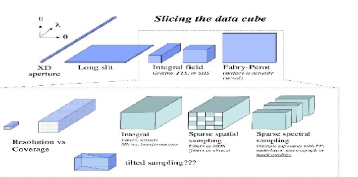
Figure 1: Sampling the data-cube with equal volumes and detector elements.

In addition to balancing the trade-offs between spatial versus spectral information, there is also the issue of balancing sampling (i.e., resolution) versus coverage in either of these dimensions. Science-driven trades formulate any specific instrument design. When sampling spatial and spectral domains, not all data has equal information content. Hence one may also consider integral versus sparse sampling. Fiber-fed IFS such as Hexaflex (Arribas, Mediavilla & Rasilla 1991) and SparsePak (Bershady et al. 2004) are examples of sparse-sampling in the spatial domain. Multi-exposure Fabry-Perot observations, multi-beam spectrographs, or notch-gratings (discussed below) are examples of instruments with the capability of sparse sampling in the spectral domain.

2 Merit Functions

There are a number of generic merit functions found in the instrumentation literature, in a variety of guises used, or tailored, to suit the need of comparing or contrasting the niche of specific instruments. Some useful preliminary definitions (used throughout this Chapter) are the spectral resolution, $R=\lambda/d\lambda$; the number of spectral resolution elements, $N_{R}$; spectral coverage = $\Delta\lambda=N_{R}\times d\lambda$; spatial resolution $d\Omega$, i.e., the sampling element on the sky (fiber, lenslet, slicer slit-let, or seeing-disk); number of spatial resolution elements, N_Ω; and spatial coverage $\Omega=N_{\Omega}\times d\Omega$.

With these definitions, the trade-offs discussed above may be summarized by stating that $N_{R}\times N_{\Omega}$ must be roughly constant for a given detector. Another important statement is that $A\times\Omega$, or grasp, is conserved in an optical system ($A$ is the telescope collecting area): The same instrument has the same $A\times\Omega$ on any diameter telescope with the same focal ratio – something derived from the identify $\Omega=a/f^{2}$, where $a$ is the instrument focal area and $f$ the focal-length. What changes with aperture, of course, is the angular sampling. For sufficiently extended sources, angular sampling is not necessarily at a premium. Imagine, for example, dissecting nearby galaxies with a MUSE-like instrument on a 4m or 1m-class telescope. (MUSE is discussed later in this Chapter; Bacon et al. 2004).

In addition to the basic ingredients listed above, the most common merit functions are the grasp, the specific grasp, $A\times d\Omega$ (how much is grasped within each spatial resolution element of the instrument), and etendue, $A\times\Omega\times\epsilon$, where $\epsilon$ is the total system efficiency from the top of the atmosphere to the detected photo-electron. Etendue is more fundamental than grasp since high-efficiency instruments are the true performance engines. Despite the fact that an instrument with an un-reported efficiency is much like a car sans fuel-gauge or speedometer, recovering $\epsilon$ from the literature is often not possible. For this reason we resort to grasp, but note that in some cases this gives an unfair comparison between instruments.

If there is no premium on spatial information then “spectral power,” $R\times N_{R}$, is suitable. At the opposite extreme, where spatial information is paramount, a suitable merit function is $A\times d\Omega^{n}\times N_{\Omega}=A\times d\Omega^{n-1}\times\Omega$, where n = 1 for high specific grasp and -1 for high resolution. In the context of 3D spectroscopy, merit functions which combine spatial and spectral power are appropriate: $\Omega\times R$, $A\times\Omega\times R\times\epsilon$, or their counterparts replacing $\Omega$ with $d\Omega$. If any information will do, $N_{R}\times N_{\Omega}$ alone gives a good synopsis of the instrument power since this effectively gives the number of resolution elements (related to detector elements) that have been effectively utilized by the instrument.

An attempt at a grand merit function can be formulated by asking the following, sweeping question: How many resolution elements can be coupled efficiently to the largest telescope aperture (A) covering the largest patrol field ($\Omega_{s}$) for as little cost as possible? In this case, the figure of merit may be written:

$$F.O.M.=\epsilon\times(\Delta\lambda/\lambda)\times(\Omega/d\Omega)\times A\times\Omega_{s}\times\pounds^{-1}\ =\ \epsilon\times N_{R}\times N_{\Omega}\times A\times\Omega_{s}\times\pounds^{-1}$$

where $\Delta\lambda$ is the sampled spectral range, and £ is the cost in the suitable local currency. To this figure of merit one may add the product $R^{n}\times d\Omega^{m}$, where $n,m=1$ if resolution is science-critical in the spectral and spatial domains (respectively), $n,m=-1$ if coverage is science-critical, or $n,m=0$ if resolution and coverage are science-neutral (in which case you’re not trying hard enough!).

From this discussion it is clear that a suitable choice of merit function is complicated, and must be science driven. The relative evaluation of instruments cannot be done sensibly in the absence of a science-formulated F.O.M.; the outcome of any sensible evaluation will therefore depend on the science-formulation. For this reason, when we compare instruments we strategically retreat and explore the multi-dimensional space of the fundamental parameters of spatial resolution, spectral resolution, specific grasp, total grasp, spectral power, and N_R versus N_Ω.

3 Why Spectral Resolution is so Important

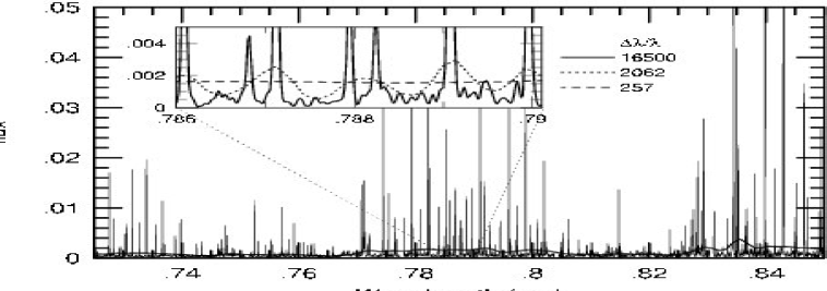
Figure 2: Night Sky near 0.8 $\mu$m at $250<R<33,000$.

In addition to the intrinsic merits and requirement of high spectral resolution for certain science programs, high resolution is of general importance for improving signal-to-noise ($S/N$) in the red and near-infrared. For ground-based observations, terrestrial backgrounds from 0.7-2.2 microns suffer a common malady of being dominated by extremely narrow (m s^-1) air-glow lines, typically from OH molecules. Unlike the thermal IR, however, there is a cure to lower the background without going to high-altitude or space. The air-glow lines cluster in bands, and the lines within the bands may be separated at $R=$3000-5000. This means that at these resolutions, while the mean background level within the spectral band-pass is constant, the median drops precipitously: more spectral resolution elements are at lower background level in inter-line regions. The lines themselves, however, remain unresolved until $R\sim$ few $\times\ 10^{5}$, so that above $R=4000$ one continues to increase the fraction of the spectral band-pass at low-background levels.

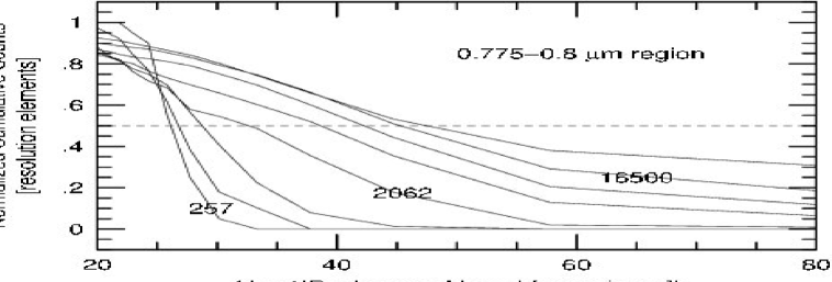
Figure 3: Cumulative distribution of resolution elements as a function of the background level proportional to $S/N$ (increasing to left) for $250<R<33,000$ (labeled).

As an illustration, we show the terrestrial sky bacgkround in a spectral region at 0.8 microns observed by D. York and J. Lauroesch (private communication) with the KPNO 4m echelle. In Figure 1.2 the sky spectra, observed at an instrumental resolution of 33,000, is degraded to illustrate the resulting change in the distribution of background levels. In Figure 1.3, the normalized, cumulative distribution of resolution elements as a function of background level are plotted for different instrumental resolutions. For background-limited measurements, the $S/N$ is proportional to the inverse square-root of the background level. Hence the median background level gives an effective scaling for sensitivity gains with spectral resolution. It can be seen the largest changes in the median background level occur between $1000<R<4000$, but significant gains continue at higher resolution. The result can be qualitatively generalized to other wavelengths in the 0.7-2.2 $\mu$m regime. While the lines become more intense moving to longer wavelengths, the power-spectrum (in wavelength) of the lines appears roughly independent of wavelength in this regime (cf. Maihara et al. 1993 and Hanuschik 2003). Note this is a qualitative assessment that should be formally quantified.

4 The Detector Limit-II: Read-noise

Our infatuation with spectral resolution is a problem given the modern predilection for high angular resolution. After the Hubble Space Telescope there is no turning back! There is, however, a limit, due to detector noise, which we always want to be above. The goal is to be photon-limited (either source or background) because this is fundamental (it’s the best we can do), and for practical purposes, $S/N$ is independent of sub-exposure time and detector sampling.

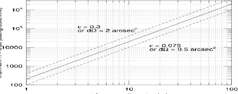
Figure 4: Maximum spectral resolution versus telescope diameter to stay background (vs detector) limited for different assumptions of instrument efficiency ($\epsilon$) and spatial sampling ($d\Omega$). The solid line assumes $\epsilon=0.15$ and $d\Omega=1$ arcsec².

To stay photon-limited in the background-limited regime puts significant constraints on the $\Omega$-R sampling unit. The spatial and spectral sampling unit can’t be too fine for a given $A$ and $\epsilon$. For 8m- and 4m-class telescopes we calculate

$$R/d\Omega < 16500(D_{T}/9m)^{2}(t/1h)(\epsilon/0.15)\ arcsec^{-2},\ {\rm or}$$

$$< 2500(D_{T}/3.5m)^{2}(t/1h)(\epsilon/0.15)\ arcsec^{-2},$$

where $D_{T}$ is the telescope aperture diameter and $t$ the (single destructive-read) exposure length. The general case is shown in Figure 1.4. To reach spectral resolutions well above $R=5000$, which is advantageous for background-reduction, a telescope significantly in excess of 10m is needed for apertures significantly under 1 arcsec^-2.

With these considerations in mind, in the next three sections (§1.2-1.4) we turn to approaches and examples of existing instruments, followed by three sections (§1.5-1.7) in which we summarize the range of these instruments, what parameter space is under-sampled, and the prospects for future instruments. Throughout, we attempt to provide relatively complete instrument lists. No doubt some instruments have been over-looked, plus the field of instrumentation advances rapidly. Reports of additional instruments or corrections are welcome.

2 Grating-Dispersed Spectrographs

Basic spectrograph theory and design can be found in most standard optics textbooks. Of particular note is the excellent monograph on astronomical optics by Schroeder (2000). In §1.2.1 we summarize the salient features to provide a consistent nomenclature, and to put these features into context of our discussion of 3D spectroscopy, specifically what drives consideration of merit functions that tune spatial versus spectral performance. The balance of this section includes a description of dispersive elements (§1.2.2), coupling methods and modes (§1.2.3-11), and summary considerations – including a discussion of sky-subtraction problems and solutions (§1.2.12).

1 Basic Spectrograph Design

In a 3D spectrographic system, there is a premium on packing spatial information onto the detector. To achieve sufficient spectral resolution at the same time requires balancing the trades between system magnification and dispersion. Starting with the grating equation, generalized for a grating immersed in medium of index $n$: $m\ \lambda=n\ \Lambda_{g}(sin\ \beta+sin\ \alpha)$, where $\Lambda_{g}$ is the projected groove separation in the plane of the grating, $m$ the order, and $\alpha$ and $\beta$ the incident and diffracted grating angles relative to the grating normal in the medium, we can write the angular and linear dispersion as $\gamma\equiv d\beta/d\lambda=m\ /\ n\ \Lambda_{g}\ cos\ \beta=(sin\ \beta+sin\ \alpha)\ /\ \lambda\ cos\ \beta$, and $dl/d\lambda=f_{2}\gamma$. Figure 1.5 illustrates a basic spectrograph, defines these angles and subsequent terms.

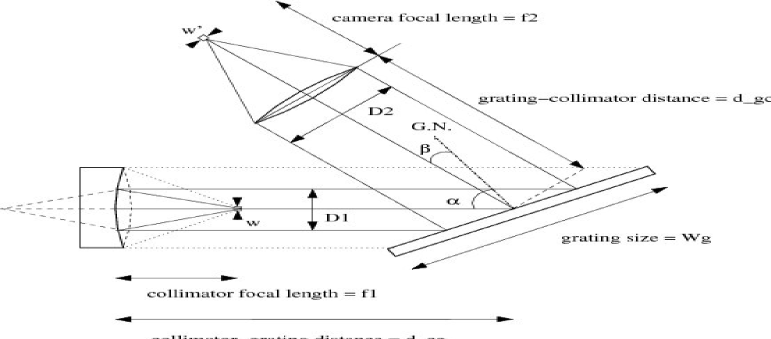
Figure 5: Basic spectrograph layout schematic for reflective/refractive collimator, reflection grating and refractive camera.

The system magnification can be broken down into spatial and anamorphic factors. The physical entrance aperture width, $w$, is re-imaged onto the detector to a physical width $w^{\prime}$, demagnified by the ratio of camera to collimator focal lengths. Hence the spatial width (perpendicular to dispersion) is given as $w_{\theta}^{\prime}=w(f_{2}/f_{1})$. For non-imaging feeds (i.e., fibers or lenslets), it is advantageous to pack as much information as possible into a given pixel – as long as individual spatial entrance elements can be resolved. This means cameras must be as fast as possible, relative to their collimators. For imaging feeds (slits or slicers), the desire to preserve and sample the spatial information retained in the slit means the choice must be science-driven.

In the dispersion direction, an additional, anamorphic factor, $r$, arises due to the fact that grating diffraction implies incident and diffracted angles need not be the same. Hence incident and diffracted beam sizes scale as $r=D_{1}/D_{2}=cos\ \alpha\ /\ cos\ \beta$. This arises because in general $A\times\Omega$ is conserved; if the beam gets larger, the angles get smaller. Another way to think of this is in terms of the definition of $r=|d\beta/d\alpha|$, and ask: For a given d$\alpha$ (angular slit width) what is d$\beta$ such that d$\lambda=0$? This result can then be derived from the grating equation. In any case, $\beta/\alpha>1$ implies magnification, while $\beta/\alpha<1$ implies demagnification. The re-imaged slit-width in the spectral dimension is then $w_{\lambda}^{\prime}=rw_{\theta}^{\prime}$. In Littrow configurations, important below, $\alpha=\beta=\delta$ (the latter being the grating blaze angle), and so there is no anamorphic factor. Since the re-imaged slit-width always degrades the instrumental spectral resolution, it is always advantageous, in this sense, to have anamorphic demagnification. However, depending on the pixel sampling, optical aberrations, and slit size, $w_{\lambda}^{\prime}$ may not be the limiting factor in instrumental resolution. Anamorphic demagnification also comes at a cost: The camera must be large (larger than the collimator) to capture all of the light in the expanded beam. Demagnification never hurts resolution, but the cost should be weighed against the gains.

The spectral resolution can now be written as $R=\lambda/d\lambda$, or $R=\lambda(\gamma/r)(f_{1}/w)$. The term $\gamma/r$ indicates we want large dispersion, but that we can get resolution also from anamorphic demagnification. The terms $f_{1}/w$ indicates we want a long collimator at fixed camera focal-length, requiring a field lens or white-pupil design to avoid vignetting. Alternatively, we may re-write the equation as $R=\lambda(\gamma/r)(D_{1}/\theta D_{T})$ noting $\theta$ is the angle on the sky, $d\lambda=w_{\lambda}^{\prime}/(dl/d\lambda)$, $w=f_{T}\theta$, and $f_{1}/d_{1}=f_{T}/D_{T}$, where $f_{T}/D_{T}$ refer to the effective focal-ratio of whatever optics feed the spectrograph, e.g., the telescope. The combination of $r$ and $D_{1}$ indicates we want a larger collimator and an even larger camera. Using the grating equation we may write $R=(f_{1}/w)(sin\ \beta+sin\ \alpha)/cos\ \alpha$, which, in Littrow configurations reduces to $R=(f_{1}/w)\ 2\ tan\ \alpha$. In the latter situation it is clear that resolution can be dispersion-driven by going to large diffraction angles, $\alpha$, which requires large gratings.

2 Dispersive Elements

We distinguish here principally between reflection and transmission gratings. Transmission gratings yield much more compact spectrograph geometries. This leads to less vignetting and better performance with smaller optics.

Reflection gratings come in three primary varieties: ruled surface-relief (SR), holographically-etched SR, or volume-phase holographic. We list the pros and cons of each of these. (i) Ruled SR gratings have the advantage of control over the groove shape, blaze and density, which provides good efficiency in higher orders (e.g., echelle) at high dispersion. There are existing samples of masters with replicas giving up to 70% efficiency, but 50-60% efficiency is typical, with 40% as coatings degrade. Scattered light and ruling errors can be significant, and existing masters are limited in type and size. It does not appear to be possible to make larger masters with high quality at any reasonable cost. (ii) Holographically etched SR gratings have low scattered light, the capability to achieve high line-density (hence high dispersion), and large size. However, they have low efficiency ($<$50%) because symmetric grooves put equal power in positive and negative orders. (iii) Volume-phase holographic gratings can be made to diffract in reflection (Barden et al. 2000), but have not yet been well-developed for astronomical use. Reflection gratings can be coupled to prisms to significantly enhance resolution via anamorphing (Wynne 1991).

Transmission gratings are either SR or volume-phase holographic, and when coupled with prisms are referred to as grisms. (i) SR transmission gratings and grisms are efficient at small angles and low line-densities (good for low-resolution spectroscopy), but are inefficient at large angles and line-densities due to groove-shadowing. Transmission echelles do exist, but have 30% diffraction efficiencies or less. (ii) VPH gratings and grisms are virtually a panacea. They are efficient over a broad range of line-densities and angles. Any individual grating is also efficient over a broad range of angles, (what is known as a broad “superblaze” – see below). Peak efficiencies are as high as 90%; they are relatively inexpensive to make, and likewise to customize; and they can be made to be very large (as larger as your substrate and recording beam – now approaching 0.5m). Their only disadvantages is that they have, to date, been designed for Littrow configurations.

It is worth dwelling somewhat on the theory and subsequent potential of VPH gratings. There still remain manufacturing issues of obtaining good uniformity over large areas (Tamura et al. 2005), but it is reasonable to be optimistic that refinement of the process will continue at rapid pace. Application in the near-infrared (NIR) for cryogenic systems is also promising: CTE mismatch between substrate and diffracting gelatin, potentially causing delamination, does not appear to be a concern (W. Brown, private communication, this Winter School). Blais-Ouellette et al. (2004) have confirmed that diffraction efficiency holds up remarkably well at 77K, but that the effective line-density changes with thermal contraction. We can expect most grating-fed spectrographs in the future will use VPH gratings alone or in combination with conventional (e.g., echelle) gratings. The capabilities of VPH gratings will open up new design opportunities, many of which will be well suited to 3D spectroscopy.

3 VPH Grating Operation and Design

Diffraction arises from modulation of the index of refraction in a sealed layer of thickness $d$ of dichromated gelatin (the material is hygroscopic), with mean optical index $n_{2}$. Typical values for $n_{2}$ are around 1.43, but the specific value depends sensitively on the modulation frequency (i.e., the line density $\Lambda$) and amplitude, $\Delta n_{2}$, and the specifics of the exposure and developing process. (Note that it is not currently possible to predict the precise value of $n_{2}$ from a manufacturing standpoint.) The seal is formed typically by two flat substrates, but this can be generalized to non-flat surfaces and wedges (i.e., prisms). Because this layer represents a volume ($d\gg\lambda$), the diffraction efficiency is modulated by the Bragg condition: $\alpha=\beta$. These angles are defined here with respect to the plane of the index modulations.

The wonder of VPH gratings is the ability to custom design them. Starting with a science-driven choice of dispersion and wavelength, the grating equation and dispersion relation given the Bragg condition uniquely set the line-frequency and angle, respectively – for unblazed gratings. The key to high diffraction efficiency is then to tune the gelatin thickness and index modulation amplitude such that diffraction efficiency is high in both s and p-polarizations (the s-polarization electric vector is perpendicular to the fringes). This can be done by brute force via rigorous coupled wave calculations, or by noting that in the so-called “Kogelnik limit” the diffraction efficiencies are periodic in these quantities (Barden et al. 2000; Baldry et al. 2004). The two polarizations have different periodicities, i.e., VPH gratings are in general highly polarizing, so the trick is finding the ($d,\Delta n_{2}$)-combination that phases one pair of s and p efficiency-peaks. Thinner gel layers yield broader band-width over which the diffraction-efficiency is high – relative to the efficiency at the Bragg condition. The thinner the layer, the larger the index modulation required to keep the efficiency high in an absolute sense. Modulations above 0.1 are very difficult to achieve, and more typical values are in the range of 0.04 to 0.07; gel layers are in the range of a few to a few 10’s of microns. In practice, because there is limited manufacturing control over the index modulation and effective depths of the gelatin exposure, gratings requiring very precise values in these parameters will be difficult to make, and have large inhomogeneities. Our experience is that it is useful to understand how wavelength and resolution requirements can be relaxed to locate more robust design-parameters.

Blazed VPH Gratings

Nominally the fringe plane is parallel to the substrate normal (indicated by the angle $\phi=0$). This yields an unblazed transmission grating. Essentially all astronomical VPH gratings in use are made this way. There is concern that tilted fringes will curve with the shrinkage of the gelatin during development (Rallison & Schicker 1992), but this concern has not been fully explored. By tilting the fringes (this is done simply by tilting the substrate during exposure in the hologram), one can enter several different interesting regimes, as illustrated concisely by Barden et al. (2000; see their Figure 1): small $|\phi|$ yields blazed reflection gratings, $\phi=90$ deg produces unblazed reflection gratings, and large $|\phi|$ blazes the reflection gratings. “Large” and “small” depend on the angle of incidence, as illustrated below. The sign convention is such that positive $\phi$ decreases the effective incidence angle. The incident and reflected angles in the gelatin, $\alpha_{2}$ and $\beta_{2}$, are related by $\alpha_{2}=\beta_{2}+2\phi$, with $\alpha_{2}-\phi$ being the effective diffraction angle. The grating equation, when combined with the Bragg condition yields: $m\ \lambda_{b}\ =\ 2\ n_{2}\ \Lambda\ sin\ (\alpha_{2}-\phi)$, where $\lambda_{b}$ is the Bragg wavelength, and $\Lambda=\Lambda_{g}\ cos\ \phi$ is the fringe spacing perpendicular to the fringes. We use Baldry et al.’s (2004) nomenclature; their Figure 1 is an instructive reference for this discussion.

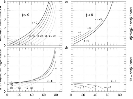
Figure 6: Resolution merit function and anamorphic factor for blazed VPH gratings with mean gel index n${}_{2}=1.43$. Typical SR gratings have $1.05<1/r<1.2$.

Baldry et al. work out the case for no fringe tilt with flat or wedged substrates. Here we give the case of flat substrates but arbitrary $\phi$. Burgh et al. (2007) extend this to include arbitrary fringe tilt. The relevant angles with respect to the grating normal can be found with these equations in terms of the physical grating properties:

$$sin\ \alpha\ =\ n_{2}\ sin\ \alpha_{2},\ \ {\rm and}\ \ \ sin\ \beta\ =\ n_{2}\ sin[\ sin^{-1}(\frac{sin\ \alpha}{n_{2}})-2\phi\ ].$$

The anamorphic factor and dispersion are still defined in terms of $\alpha$ and $\beta$ as given in §1.2.1. With the interrelation of these angles as given above, it is easy to show the logarithmic angular dispersion at the Bragg wavelength is:

$$d\beta/dlog\lambda=2\ n_{2}\ cos\ \phi\ sin[\ sin^{-1}(\frac{sin\ \alpha}{n_{2}})-\phi]\ /\ cos\ \beta.$$

To understand the potential advantages of blazed transmission gratings, we define a resolution merit function as $\frac{1}{r}\ d\beta/dlog\lambda,$ i.e., the product of the logarithmic angular dispersion and the anamorphic factor. With this function we can explore, in relative terms, if tilting the fringes yields resolution gains. Figure 1.6 shows the anamorphic factor and the resolution merit function versus grating incidence angle for positive and negative fringe-tilts. Negative fringe tilts give a small amount of increased resolution at a given $\alpha$ by significantly increasing dispersion, which over-comes an increase in the anamorphic magnification. This means the detector is less efficiently used. Negative fringe tilts also limit the usable range of $\alpha$ for which $\beta<90$ deg (transmission), and hence the maximum achievable resolution in transmission that can be achieved is lowered with negative fringe tilts.

With positive fringe tilts, the anamorphic demagnification increases strongly at large incidence angles, although there is little gain in going to $\phi>15$ deg. Note that the demagnification becomes $<1$ (i.e., magnification) roughly when $\alpha\sim 1.5\ \phi$. This is when the effective diffraction angle ($\alpha_{2}-\phi$), changes sign with respect to the tilted fringes (the grating remains in transmission). The overall resolution decreases with increased positive fringe tilt, but the decrease is modest for small tilt angles. Given the large increase in anamorphic demagnification relative to the modest loss in resolution, for small tilt angles there is a definite gain in information: A +5 deg tilt gives a 12% loss in the resolution merit function at $\alpha=60$, but a 51% gain in the anamorphic demagnification. With suitably good optics and detector sampling the demagnified image, this equates directly into an increase in the number of independent spectral resolution elements, replete with a 72% increase in spectral coverage. The loss in resolution can easily be made up by slightly increasing $\alpha$ (in this case, from 60 to 63 deg) and modulating $\Lambda$ in the grating design to tune the wavelength. Instruments with blazed, high-angle VPH gratings with tilts of $5<\phi<15$ deg will allow for the high resolution needed to work between sky-lines, while efficiently packing spectral elements onto the detector. This is critical in the context of 3D spectroscopy, where room must also be made for copious spatial elements.

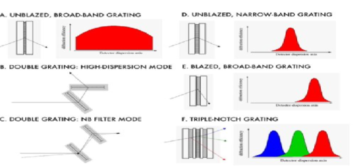
Figure 7: Novel grating modes. A. Conventional broad-band application now becoming a staple of modern spectrographs. B. Double-grating geometry yielding a net dispersion of $\sim$ the sum of the two individual grating dispersions (gratings are not necessarily identical, but angles must be adjusted accordingly). C. Double-grating geometry yielding a narrow-band filter with field-dependent band-pass given by the Bragg condition (gratings are identical) D.-F. Narrow band-pass gratings unblazed (D), blazed (E), and combined (F) to form a notch grating. Other modes are discussed in the text. Panels A, D-F show both the grating configuration as well as a cartoon-sketch of the diffraction efficiency as a function of location of the detector dispersion axis, labeled for the mean wavelength regime of the diffraction band-pass.

Unusual VPH Grating Modes

In addition to tilted fringes, VPH gratings pose opportunities for a number of novel modes well suited to 3D spectroscopy. Figure 1.7 illustrates some of these. With very high diffraction efficiency it is now reasonable to consider combining gratings to augment the dispersion, and hence resolution. If the two gratings are kept parallel but offset along the diffraction angle, they can serve as (tunable) narrow-band filters – an alternative to etalons (e.g., Blais-Ouellette et al. 2006). Barden et al. (2000) have explored using multiple gelatin layers with different line-frequencies to select H$\alpha$ and H$\beta$ in separate band-passes. By slightly rotating one set of lines, sufficient cross-dispersion is added to space the two spectra – one above the other – on the detector. This is well suited for spectrographs fed with widely spaced fibers or slitlets (i.e., an under-filled, conventional long-slit spectrograph), and represents an interesting trade-off in wavelength and spatial multiplex. At sufficiently high dispersion (and hence limited band-pass), the number of layers could be increased to mimic a multi-order echelle. The advantage of this approach is in resolution and wavelength coverage.

An alternative approach is something we refer to as “notch” gratings. Here, we take advantage of the relative ease (from a manufacturing stand-point) of achieving a narrow band-pass, and combine gel layers tuned to different, non-over-lapping wavelength band-passes at a given incidence angle (e.g., by changing the line frequency). By also tuning the fringes with with modest tilts, each band pass can be centered on a different, non-overlapping portion of the detector. Band-passes will have to be carefully crafted by tuning grating parameters to avoid parasitic contamination in the other bands. The figure illustrates positive and negative tilts, but the tilts could be arranged to all be positive to take advantage of the anamorphic factors described above. This offers another way to slice the data cube – one which allows for sparse spectral sampling of key spectral diagnostics over a broad wavelength range (e.g., [OII]$\lambda$3727, H$\beta$+[OIII]$\lambda\lambda$4959,5007, and H$\alpha$) at high dispersions, with ample room left over on the detector for significant spatial multiplex.

4 Summary of Implications for 3D Spectrograph Design

The most compact spectrograph designs yield the highest-efficiency, wide-field systems needed to grapple with attaining large angular coverage for 3D spectroscopy. To also obtain high-enough spectral resolution to work between the atmospheric air-glow often requires significant dispersive power and anamorphic demagnification. Large anamorphic demagnification, while not free (larger camera optics are required), is well-suited to packing information onto the detector. This is particularly important in 3D applications where spatial multiplex is at a premium. VPH transmission gratings are clearly preferred because they lend themselves to compact spectrograph geometry and provide high diffraction efficiency. We have shown they can, in principle, also yield large anamorphic demagnification. With high-angle, double, and blazed VPH gratings, echelle-like resolutions can be achieved at unprecedented efficiency (75-90% in diffraction alone). Unusual modes to produce tunable narrow-band filters and notch gratings also open up the possibility for well-targeted sparse, spectral sampling.

5 Coupling Formats and Methods: Overview

The essence of the 3D spectrometer lies in the coupling of the telescope focal plane to the spectrograph. We review the four principal methods: (i) direct fibers, (ii) fibers + lenslets, (iii) image-slicers, and (iv) lenslet arrays, or pupil-imaging spectroscopy. A nice, well-illustrated overview can be found in Allington-Smith & Content (1998); additional discussion of the merits and demerits of different approaches can be found in Alighieri et al. (2005). Here we also make an evaluation. We discuss a fifth mode not seen in the literature, which we refer to as (v) “filtered multi-slits.” Many spectrographs either have, or could easily be modified to have, this capability. We also describe (vi) multi-object configurations – a mode which will undoubtedly become more common in the future.

Throughout this discussion, we distinguish between near-field versus far-field effects. The near-field refers to the light distribution at the focal surface, e.g., fiber ends, and what is re-imaged ultimately onto the CCD. The far-field refers to the ray-bundle distribution, i.e., the cross-section intensity profile of the spectrograph beam significantly away from the focal surface. Different coupling methods offer the ability to remap near- and far-field light-bundle distributions, which can have advantages and dis-advantages.

6 Direct Fiber Coupling

The simplest and oldest of methods consists of a glued bundle of bare fibers mapping the telescope to spectrograph focal surfaces. With properly doped, AR-coated fibers throughput can be at or above 95%, which can be compared to 92% reflectivity off of one freshly coated aluminum surface. These have the distinct advantage of low cost and high throughput. As with all fiber-based coupling, there is a high degree of flexibility in terms of reformatting the telescope to spectrograph focal-surfaces (for example, it is easy to mix sky and object fibers along slit), and the feeds can be integrated into existing long-slit, multi-object spectrographs. However, bare fiber IFUs are not truly integral, and do not achieve higher than 60-65% fill-factors (see Oliveria et al. 2005 on the deleterious effects of buffer-stripping of small fibers). This coupling is perhaps the most cost-effective mode for cases where near-integral sampling is satisfactory, and preservation of spatial information is not at a premium.

Information loss and stability gain with fibers: Focal Ratio Degradation (FRD) and azimuthal scrambling represent information loss (an entropy increase). FRD specifically results in a faster output f-ratio (Ramsey 1988). This has an impact on spectrograph design or performance since either the system will be lossy (output cone over-fills optics), or the spectrograph has to be designed for the proper feed f-ratio. PMAS (Roth et al. 2005) is an excellent example of how to properly design a spectrograph to handle fast fiber-output beams. The existing WIYN Bench spectrograph is a good example of how not to do it. In fact, it’s so bad we rebuilt it (Bershady et al. 2008); we were able to recapture 60% of the light (over a factor of 2 in throughput) with no loss of spectral resolution in the highest-resolution modes.

Azimuthal scrambling can help and hurt. While scrambling destroys image information, it symmetrizes the output beam, ameliorating, to some extent, the effect of a changing telescope pupil on HET or SALT-like telescopes by homogenizing the ray bundle. Thus, the contribution of spectrograph optical aberrations to the final spectral image is more stable. (This is a far-field effect.)

Radial and azimuthal scrambling together homogenize near-field illumination, e.g., the seeing-dependent slit function is decreased. Radial scrambling and FRD are one and the same (cf. Ramsey 1988 and Barden et al. 1993), so that one trades information loss for stability (similar to the trade of precision for accuracy). In practice, fiber-input beam-speeds of f/3 (PMAS) to f/4.5 (HET and SALT) are desirable. However, with fast input/output f-ratios this limits possible spectrograph demagnification since it is expensive to build faster than f/2 for large cameras.

Telecentricity. Because azimuthal scrambling symmetrizes a beam, if the input light-cone is mis-aligned with the fiber axis, the output beam (f-ratio) is faster. This is not FRD. To avoid this effect, fiber telecentric alignments of under a degree are needed even for f-ratios as fast as 4-6 (Bershady 2004, Wynne & Worswick 1989).

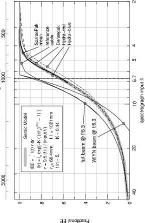
Figure 8: Output fiber irradiance (encircled-energy versus beam f-ratio) for fiber cables on the WIYN Bench Spectrograph. The input beam profile is an unappodized f/6.3 beam with an f/17 central obscuration (labeled). Output beam profiles are faster, due to FRD, and are well-fit by a Sersic model of index 1/n = 5 (S. Crawford, private communication).

Causes of FRD. Excessive FRD in fibers is due to stress. Hectospec (Fabricant et al. 2005) embodies an excellent example of how to properly treat fibers and fiber cabling (Fabricant et al. 1998; see also Avila et al. 2003 in the context of FLAMES on VLT). Fiber termination and polishing can also induce stress. Bershady et al. (2004) discuss some other IFU-related issues in terms of buffering. However, even for perfectly handled fibers, there is internal scattering - the cause of which has long been a debate. Nelson et al. (1988) suggested a combination of (a) Rayleigh scattering (variation in fiber refractive index); (b) Mie scattering (fiber inhomogeneities comparable to the wavelength); (c) stimulated Raman and Brillouin scattering (not relevant at low signal level in astronomical applications); and (d) micro-bending. Micro-bending seems like a good culprit; it is the unsubstantiated favorite in the literature. Micro-bending models predict a wavelength-dependent FRD. While Carrasco & Parry (1994) tentatively see such an effect, neither Schmoll et al. (2003) or Bershady et al. (2004) confirm the result. However, these studies use different measurements methods. More work is required to understand the physical cause(s) of FRD, and with this understanding, perhaps, reduce the amplitude of the effect. We find FRD produces an output fiber beam profile which can be well-modeled by a Sersic function (Figure 1.8; S. Crawford, private communication). This either says something about the scattering model or how seriously to take physical interpretations of Seric-law profiles of galaxies!

Figure 9: Critical sampling with densely-packed fibers.

Quality versus quantity: Fibers offer the opportunity of easily trading quality for quantity in terms of packing the spectrograph slit. Scattered light within the spectrograph, combined with fiber azimuthal-scrambling means spatial information in the telescope focal plane is coupled to all adjacent fibers in the slit. Closely packing fibers in the slit can make clean spectral extraction difficult. The WIYN Bench spectrograph is a good example where the amplitude of scattered light is low, fiber separation is large and ghosting is negligible. This spectrograph and feeds are optimized for clean extraction with little cross-talk (1% cross-talk in visible in optimum $S/N$ aperture, degrading to 10% in the NIR). Information packing in the spatial dimension is modest due to fiber separation, while information packing in the spectral dimension is high due to large anamorphic factors. Other systems have significant spectral overlap. For example, staggered slits, where fibers are separated by only their active diameter (COHSI; Kenworthy et al. 1998) make it difficult to extract a clean spectrum and optimize $S/N$ at the same time, but the spatial multiplex is increased. There is no one right answer, but definitely a decision worthy of a science-based consideration.

Image reconstruction and registration. Even without lenslets, densely sampled fibers provide excellent image reconstruction on spatial scales of order the fiber diameter. One can achieve the theoretical sampling-limit with a 3-position pattern of half-fiber-diameter dithers (Figure 1.9; cf. Koo et al. 1994 in the context of under-sampled HST/WFPC-2 data). Even with sparse sampling, registration of the spectral data-cube with broad-band images can be achieved to 10% of the fiber diameter by cross-correlating the spectral continuum with respect to broad-band images or integrated radial light profiles (Bershady et al. 2005). Kelz et al. (2006) show how well it is possible to reproduce the continuum image of UGC 463 using the PPak fiber bundle – without any sub-sampling.

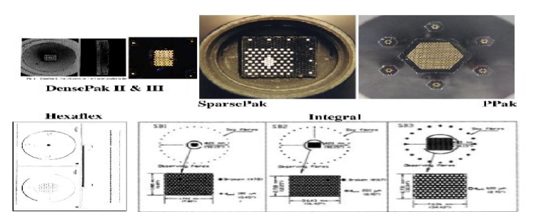
Figure 10: Direct-fiber IFUs on optical spectrographs. The top row shows the legacy started by S. Barden with DensePak-1 and DensePak, leading to SparsePak, PPaK on the KPNO 4m, WIYN, and Calar Alto, respectively; the bottom row shows Hexaflex and Integral on WHT with their multiple, selectable bundles and ample sky-fibers.

Summary of instruments. Some of the first IFUs were on the KPNO 4m RC spectrograph: DensePak-1 followed by DensePak-2 (Barden & Wade 1988; see also Guerrin & Felenbok 1988 for other early IFUs). The last incarnation (Barden et al. 1998) was on WIYN. Conceptually, these instruments spawned SparsePak (WIYN; Bershady et al. 2004) and PPak (PMAS, Calar Alto, Verheijen et al. 2004; Kelz et al. 2006). A more-versatile single instrument-suite, built for the WHT, is INTEGRAL (WYFFOS), which offers several plate-scales and formats (Arribas et al. 1998), and a sophisticated and well thought-out mapping between telescope and spectrograph focal planes. These are all shown in Figure 1.10. GOHSS is one case of a NIR (0.9-1.8$\mu$m) application (Lorenzetti et al. 2003). VIRUS (Hill et al. 2004) and APOGEE (Allende Prieto et al. 2008) are the only planned future instruments.

Table 1: Direct Fiber-Coupled Integral Field Instruments

Instrument	Tel.	DT	$\Omega$	d$\Omega$	NΩ	$\Delta\lambda/\lambda$	R	NR	$\epsilon$
		(m)	(arcsec2)
Existing Optical Instruments
DensePak	WIYN	3.5	564	6.2	91	1.02	1000	1024	0.04
		3.5	564	6.2	91	0.07	13750	1024	0.04
		3.5	564	6.2	91	0.04	24000	1024	0.04
		3.5	119	1.3	91	1.02	1000	1024	0.04
		3.5	119	1.3	91	0.07	13500	1024	0.04
		3.5	119	1.3	91	0.04	24000	1024	0.04
SparsePak	WIYN	3.5	1417	17.3	82	1.02	800	819	0.07
		3.5	1417	17.3	82	0.07	11000	819	0.07
		3.5	1417	17.3	82	0.03	24000	819	0.07
PPak	CA	3.5	2070	5.64	367	0.15	7800	1183	0.15
INTEGRAL	WHT	4.2	32.6	0.159	205	0.22	2350	515	$\cdots$
		4.2	32.6	0.159	205	0.94	550	515	$\cdots$
		4.2	139.3	0.64	219	0.22	2350	515	$\cdots$
		4.2	139.3	0.64	219	0.94	550	515	$\cdots$
		4.2	773	5.73	135	0.07	2350	300	$\cdots$
		4.2	773	5.73	135	0.90	550	300	$\cdots$
Future Optical Instruments
VIRUS	HET	9.2	32604	1.0	32604	0.505	811.	410	0.16
Existing Near Infrared Instruments
GOHSS	TNG	3.6	44.2	1.77	25	0.12	4380.	512	0.13
Future Near-Infrared Instruments

7 Fiber + Lenslet Coupling

The basic concept of lenslet coupling to fibers is again, as with bare fibers, to remap a 2D area in the telescope focal-surface to a 1D slit at the spectrograph input focal surface. The key difference is in the fore-optics, which consists of a focal expander and lenslet array; these feed the fiber bundle. The focal expander serves to matches to the scale of the lenslet array. Allington-Smith & Content (1998) and Ren & Allington-Smith (2002) present some technical discussion and illustration of the method. Each micro-lens in the array then forms a pupil image on the fiber input face. The pupil image is suitably smaller than the lenslet to allow the fibers to be packed behind the integral lenslet array. This reduction speeds up the input beam ($A\times\Omega$ is conserved). Given the previous discussion concerning FRD, this can be advantageous to minimize entropy increase.

At the output stage, the option exists to reform the (now azimuthally scrambled) slit-image with an output micro-lens linear array, or to use bare fibers. Without lenslets, the input f-ratio to the spectrograph will be faster, which means there is less possibility for geometric demagnification via a substantially faster camera. In this case the spectrograph also reimages the fiber-scrambled telescope pupil: the image varies with telescope illumination, while the ray-bundle distribution (far-field) varies with the telescope image.

The positive attributes of lenslet-fed fiber arrays are: (i) improved filling factors to near unity; and (ii) control of input and output fiber f-ratio. The latter permits effective coupling of a slow telescope f-ratio to fiber input at a fast, non-lossy beam speed, and likewise, permits effective coupling of fiber output to spectrograph. The negative attributes of this coupling method include (iii) increased scattered light (from the lenslet array); (iv) lower throughput (due to surface-reflection, scattering, and misalignment). For example, typical lenslet + fiber units yield only 60-70% throughput (Allington-Smith et al. 2002). When there is a science premium on truly integral field sampling, the above two factors don’t out-weigh the filling factor improvements. Finally, there is the more subtle effect of whether or not to use output lenslets. Aside from the matter of f-ratio coupling, there is the issue of whether swapping the near- and far-field patterns is desirable for controlling systematics in the spectral image. It amounts to assessing whether the spectrograph is “seeing-limited”, i.e., limited by spatial changes in the light distribution within the slit image formed by the fiber and lenslet, or aberration limited?

Prime examples of optical instruments on 8m-class telescopes include VIMOS (Le Fevre et al. 2003), GMOS (Gemini-N,S, Allington-Smith et al. 2002), and FLAMES/GIRAFFE in ARGUS or multi-object IFU modes (Avila et al. 2003). Typical characteristics of these devices is fine spatial sampling (well under an arcsec) and modest spectral resolution. ARGUS is an exception, achieving resolutions as high 39,000. It’s multi-object mode is also unique – and powerful (see later discussion). On 4m-6m class telescopes there are PMAS (Roth et al. 2005), Spiral+AAOmega (Saunders et al. 2004, Kenworthy et al. 2001), MPFS (Afanasiev et al. 1990), and IMACS-IFU (Schmoll et al. 2004). Compared to most direct-fiber IFUs on comparable telescope, these instruments also have finer spatial sampling.

Table 2: Fiber+Lenslet Coupled Integral Field Instruments

Instrument	Tel.	DT	$\Omega$	d$\Omega$	NΩ	$\Delta\lambda/\lambda$	R	NR	$\epsilon$
	Method	(m)	(arcsec2)
Existing Optical Instruments
PMAS	Calar Alto	3.5	64.	0.5	256	0.11	9400	1000	0.15
		3.5	64.	0.5	256	0.52	1930	1000	0.15
		3.5	144.	0.75	256	0.11	9400	1000	0.15
		3.5	144.	0.75	256	0.52	1930	1000	0.15
		3.5	256.	1.0	256	0.11	9400	1000	0.15
		3.5	256.	1.0	256	0.52	1930	1000	0.15
SPIRAL	AAT	3.9	251.	0.49	512	0.29	1700	495	0.25
		3.9	251.	0.49	512	0.07	7500	495	0.25
MPFS	SAO	6.0	256.	1.0	256	0.12	8800	1024	0.045
		6.0	64.	0.25	256	0.47	2200	1024	0.045
IMACS-IFU	Magellan	6.5	62.0	0.031	2000	0.61	2500	4096	0.19
		6.5	37.7	0.031	1200	0.31	7500	2340	0.17
GMOS	Gemini	8.0	49.6	0.04	1500	0.21	3450	730.	$\cdots$
		8.0	49.6	0.04	1500	0.32	2300	730	$\cdots$
		8.0	49.6	0.04	1500	0.82	890	730	$\cdots$
		8.0	24.8	0.04	750	0.42	3450	1460	$\cdots$
		8.0	49.6	0.04	1500	0.64	2300	1460	$\cdots$
		8.0	49.6	0.04	1500	1.00	890	1460	$\cdots$
VIMOS	VLT	8.0	2916.	0.45	6400	0.6	250	150	$\cdots$
		8.0	698.	0.11	6400	0.6	250	150	$\cdots$
		8.0	729.	0.45	1600	0.2	2500	500	$\cdots$
		8.0	174.5	0.11	1600	0.2	2500	500	$\cdots$
ARGUS/IFU	VLT	8.0	83.9	0.27	315	0.105	11000	1155	$\cdots$
		8.0	83.9	0.27	315	0.042	39000	1625	$\cdots$
ARGUS	VLT	8.0	27.7	0.09	315	0.105	11000.	1155	$\cdots$
		8.0	27.7	0.09	315	0.042	39000.	1625	$\cdots$
Future Optical Instruments
Existing Near-Infrared Instruments
COHSI	UKIRT	3.8	8.5	0.85	100	0.26	500.	128	$\cdots$
SMIRFS	UKIRT	3.8	24.2	0.34	72	0.023	5500.	128	$\cdots$
CIRPASS	Gemini	8.0	54.5	0.13	490	0.41	2500.	1024	$\cdots$
		8.0	54.5	0.13	490	0.085	12000.	1024	$\cdots$
		8.0	27.0	0.06	490	0.41	2500.	1024	$\cdots$
		8.0	27.0	0.06	490	0.085	12000.	1024	$\cdots$
Future Near-Infrared Instruments

NIR instruments include SMIRFS (Haynes et al. 1999), and COHSI, which is a precursor - in some regards - to CIRPASS (Parry et al. 2004). An interesting application of flared fibers is discussed by Thatte et al. (2000) for cryogenic systems.

A summary of existing and future optical and NIR lenslet + fiber coupled IFU spectrographs are listed in Table 2. While it may seem surprising that no future instruments appear to be planned, we will discuss one possible instrument for the 30m Telescope (TMT) below.

8 Slicer Coupling

Image-slicers have been around for a long time, primarily serving the high-resolution community, e.g., to slice a large fiber into a thin, relatively short slit to feed cross-dispersed echelle’s (see Tull et al. 1995 for one recent example). Extending the concept into a 3D mode follows the same basic notion, which can be thought of as deflecting slices of the telescope image plane both along and perpendicular to the slice through a pair of reflections. These reflections have power to reform the focal-plane image. Given the deflections, the slices are re-aligned end-to-end as in a long-slit, which then feeds a conventional spectrograph.

The latest incarnation is the so-called “Advanced Image Slicer” (AIS) concept – a 3-element system, introduced and nicely illustrated by Allington-Smith et al. (2004). In short, the slicer mirrors at the telescope focal plane divide it into strips, and have power to place the telescope pupil on the next slicer element. This is desirable to keep these elements small and the slicer compact. The second element is an array of pupil mirrors (one per slice), which reformat the slices into a pseudo-slit, where they form an image of the sky. A tertiary field lens (a lenslet for each slice) control the location of the pupil stop in the spectrograph. This is critical for efficient use of the spectrograph. All-mirror designs exist for the NIR (FISICA, Eikenberry 2004b), taking advantage of lower scattering at longer wavelengths to machine monolithic elements. Catadioptric designs exist for the optical (MUSE, Henault et al. 2004). Here the pupil lenses replace pupil mirrors, which aids the geometric layout of the spectrograph system.

The salient features of image slicers are (i) they are the only IFU mode to preserve all spatial information. All other coupling modes destroy spatial information within the sampling element, either by fiber scrambling or pupil-imaging (below). (ii) Image slicers are also the most compact at reformatting the focal plane onto the detector. (iii) They can be used in cryogenic systems and at long wavelengths where fibers don’t transmit (although lenslet arrays also accomplish this – see next section). There are some disadvantages, including (iv) scattered-light from the slicing mirrors (diamond-turned optics can’t be used in the optical), and (v) a lack of reformatting freedom. The latter is perhaps less of a concern given that the image is being preserved. However, for possible multi-object modes, particular attention must be payed to the design of the required relay optics to avoid efficiency losses.

Table 3: Slicer Coupled Integral Field Instruments

Instrument	Tel.	DT	$\Omega$	d$\Omega$	NΩ	$\Delta\lambda/\lambda$	R	NR	$\epsilon$
		(m)	(arcsec2)
Existing Optical Instruments
ESIa	Keck	10.0	22.8	1.28	18	0.95	3500	3325	0.14
		10.0	15.0	0.56	27	0.95	5200	4950	0.14
		10.0	10.0	0.25	40	0.95	7800	7410	0.14
		10.0	8.4	0.09	93	0.95	13000	12350	0.14
Future Optical Instruments
WiFeS	ANU	2.3	775.	1.	775	1.03	3000	3090	$\cdots$
		2.3	775.	1.	775	0.44	7000	3090	$\cdots$
MUSEa	VLT	8.0	3600	0.04	9e4	0.67	3000	2000	0.24
Existing Near-Infrared Instruments
UIST	UKIRT	3.8	19.8	0.06	344	0.15	3500	512	$\cdots$
PIFS	Palomar	5.0	51.8	0.45	115	0.23	550	128	0.22
		5.0	51.8	0.45	115	0.10	1300	128	0.22
NIFSa	Gemini	8.0	9.0	0.01	900	0.19	5300.	1007	$\cdots$
GNIRSa	Gemini	8.0	15.4	0.023	684	0.301	1700	512	$\cdots$
		8.0	15.4	0.023	684	0.087	5900	512	$\cdots$
SPIFFI	VLT	8.0	0.54	0.006	1024	0.34	3000	1024	0.3
		8.0	10.2	0.001	1024	0.34	3000	1024	0.3
		8.0	64.0	0.06	1024	0.34	3000	1024	0.3
Future Near-Infrared Instruments
KMOSa	VLT	8.0	188.0	0.04	4204	0.28	3600.	1000	$\cdots$
FISICAa	GTC	10.4	72.0	0.53	136	0.79	1300.	1024	$\cdots$
a Advanced Image Slicer design.

We summarize the existing and planned instruments in Table 3. The length of the list, particularly in the planned instruments marks a sea-change over the last few years away from fiber+lenslet coupling. While slicers originated for NIR instruments, starting with the now-defunct MPE-3D (Thatte et al. 1994), the list of planned optical slicers is extensive. Existing NIR instruments include PIFS (Murphy et al. 1999) and UIST (Ramsay Howat et al. 2006) on 4m-class telescopes; NIFS (McGregor et al. 2003), GNIRS (Allington-Smith et al. 2004), and SPIFFI (Eisenhauer et al. 2003, Iserlohe et al. 2004), on 8m-class telescopes. SINFONI (SPIFFI + MACAO) on VLT (Bonnet et al. 2004) in particular has shown the power of NIR adaptive-optics (AO) coupled to an image slicer at moderate spectral resolution achieving 20-30% throughput. Future NIR instruments include KMOS (Sharples et al. 2004) – a multi-object system discussed below, and FISICA. Below we also discuss three planned NIR instruments for space.

While the only existing optical instrument is ESI (Sheinis et al. 2002, 2006), future optical instruments include WiFeS (Dopita et al. 2004), SWIFT (Goodsall et al., this workshop), and MUSE (Bacon et al. 2004 and references therein). ESI is unique in being the only cross-dispersed IFU system. While the number of spatial elements is modest, ESI has enormous spectral multiplex (at medium spectral resolution and good efficiency) – the largest of any instrument planned or in existence.

9 Direct Lenslet Coupling

This is the most significant departure in grating-dispersed 3D spectroscopy, and therefore the most interesting. The basic concept consists of pupil-imaging spectroscopy using lenslets. The same type of lenslet array used in the fiber+lenslet mode create a pupil image from each lenslet, which again is smaller than the size of the lenslet. Here, the array of pupil-images forms the spectrograph input focal surface, or object; no fibers or slicers reformat the telescope focal plane into long-slit; the two-dimensional array of pupil-images is preserved. However, the pupil image does not preserve the spatial information within the lenslet field. These pupil images are dispersed, and then re-imaged at the output spectrograph image surface.

Because direct lenslet injection preserves the 2D spatial data format, this type of instrument typically offers more spatial coverage or sampling at the expense of spectral information. The extent of the spectrum from each pupil image must be truncated to prevent overlap between pupil images. From the instrument design perspective, what is gained is significant: The spectrograph field of view grows linearly with $\Omega$, instead of as $\Omega^{2}$ as it must in a long-slit spectrograph, where the 2D spatial information must be reformatted into a 1D slit. Hence this mode is best suited to instruments with the largest $\Omega$ or $N_{\Omega}$.

Lenslet-coupled instruments have excellent spatial fill factor, identical to fiber+lenslet systems, and comparable to slicers. Because this is achieved with fewer optical elements and no fibers, there is no information loss via FRD, and overall the system efficiency can be very high. As with fiber+lenslet coupling, there are concerns about scattered light from lenslets apply here too. Unlike fiber-coupled modes, there is no control over spatial re-formatting. The spectra can be well-packed onto the detector, but as noted above, the band-pass must be crafted to prevent overlap for a given spectral dispersion, i.e., there is limited spectral coverage at a given resolution. Spectral extraction is critical to minimize crosstalk while maximizing $S/N$.

Existing optical systems (SAURON, Bacon et al. 2001; OASIS, McDermid et al. 2004) have relatively low dispersion due to grism limitations, although the grisms allow for very compact, undeviated systems. Grating-dispersed systems do exists in the NIR (OSIRIS, Larkin et al 2003). Future systems with VPH grisms and gratings will have even higher efficiency; the coupling mode is well suited to articulated-camera spectrographs. The systems summarized in Table 4 are designed to exploit superb image quality with fine spatial sampling (OASIS and OSIRIS are coupled to AO). While they cannot take advantage of high dispersion without becoming read-noise limited, systems with larger specific-grasp could be optimized for high spectral resolution.

Table 4: Lenslet-Coupled Integral Field Instruments

Instrument	Tel.	DT	$\Omega$	d$\Omega$	NΩ	$\Delta\lambda/\lambda$	R	NR	$\epsilon$
		(m)	(arcsec2)
Existing Optical Instruments
SAURON	WHT	4.2	1353	0.88	1577	0.11	1213	128	0.147
		4.2	99	0.07	1577	0.10	1475	150	0.147
OASIS	WHT	4.2	1.92	0.002	1100	0.50	1000	400	$\cdots$
		4.2	31.0	0.026	1100	0.50	1000	400	$\cdots$
		4.2	180.	0.17	1100	0.50	1000	400	$\cdots$
Future Optical Instruments
Existing Near-Infrared Instruments
OSIRIS	Keck	10.4	1.2	0.02	3000	0.12	3400	400	$\cdots$
		10.4	30.	0.10	3000	0.12	3400	400	$\cdots$
		10.4	0.3	0.02	1019	0.47	3400	1600	$\cdots$
		10.4	7.5	0.10	1019	0.47	3400	1600	$\cdots$
Future Near-Infrared Instruments

10 Filtered Multi-Slit (FMS) Coupling

The notion of direct lenslet-coupling motivates a poor-person’s alternative, which returns the riches of preserving spatial information. The concept is to use a conventional, multi-object imaging spectrograph with a narrow-band filter, and a slit-mask of multi-slits in a grid pattern with grid-spacing tailored to the desired dispersion of the grating. This is illustrated in Figure 1.11. Spatial multiplexing is increased via filtering. While this only offers sparse spatial sampling, it preserves spatial information (unlike any other mode except slicing), and can easily be adapted to existing spectrographs.

The notion of filtering to increase spatial multiplex has been used for multi-object spectroscopy, e.g., Yee et al. (1996) in the context of redshift surveys using MOS on CFHT (Le Fevre et al. 1994). Likewise, fiber+lenslet coupled IFUs, such as VIMOS and GMOS, use filtering as an option to prevent spectral overlap in configurations with multiple, parallel pseudo-slits; this is designed to permit trade-offs in spatial versus spectral coverage. What is described here is more like the multi-object mode, but instead uses a regular grid of slitlets. This is well-suited, for example, to observing single, extended sources.

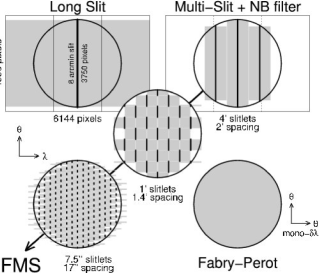
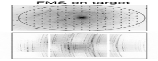
Figure 11: Filtered multi-slit schematic for SALT’s RSS. The 5 panels at left show the progression from long-slit, to filtered long-slit, to two different grids of filtered multi-slits. Both are tuned to a high dispersion, 10 nm band-pass, and achieve a spatial multiplex gain of 3 over a pure long-slit, with a 6x loss in band-pass. Higher spatial multiplex (2-10$\times$) is achieved at lower spectral resolution. The RSS Fabry-Perot mode is shown for reference. The two right-most panels show an overlay on a nearby, face-on galaxy, and some on-telescope calibration data for that slit-mask.

An example of this type of instrument is the SALT Robert Stobie Spectrograph (RSS), a prime focus imaging spectrograph with an 8 arcmin field of view, articulating camera, VPH grating suite, dual Fabry-Perot etalons, and $R=50$ order-blocking filters (Kobulnicky et al. 2003, Burgh et al. 2003). The latter can be used with the multi-slit masks to gain a factor of 3 in spatial multiplex at the highest spectral resolutions ($R=10,000$ with a 10 nm band-pass). At lower resolutions (and fixed band-pass), the slit-packing can be increased by factors of 2 to 10, such that the gain in spatial multiplex is comparable to the loss of a factor of 5-6 in spectral multiplex in this particular case (the system is designed for large spectral multiplex). Even at high spectral resolution what is gained – beyond the spatial multiplex – is the ability to gain 2D spatial mapping in a single exposure. On balance, what is lost and gained is comparable from a purely information stand-point, and hence the choice is, as always, science-driven. For the study of nearby galaxy kinematics, this is an outstanding approach.

11 Multi-object Configurations

Multi-object 3D spectroscopy is a major path for future instrumentation, although it already exists today in one fabulous instrument: FLAMES/GIRAFFE. Here we are talking about instruments with multiple, independently positionable IFUs. Returning to our so-called “grand” merit function, it is for just these types of instruments that $\Omega_{s}$ is relevant.

The most obvious way to feed such an instrument is with fiber or fiber+lenslet bundles (e.g., FLAMES/GIRAFFE). Fiber-based systems provide flexibility for spatial positioning, but for cryogenic NIR instruments, lenslets or slicers may be required. This necessitates relay optics, which are more mechanically challenging to design and build, and introduce additional surfaces which lead to lowered throughput. Sharples et al. (2004) have considered the multiple, deployable slicer design for KMOS. It is also possible to implement direct lenslet coupling (pupil imaging), as demonstrated by the MUSE concept (Henault et al. 2004), albeit in the context of splitting up a monolithic field into chunks fed to separate spectrographs.

12 Summary of Considerations

The various coupling methods discussed above present different opportunities for down-selecting information, and packing three into two dimensions in ways which trade quality versus quantity.

Information Selection and Reformatting

Fiber+lenslet, slicers, and lenslet modes yield comparable spatial telescope focal-surface sampling, while pure fiber systems have at best 65% integral coverage. Fiber-based systems, however, offer the most flexibility in re-formatting telescope to spectrograph focal surfaces. Slicers and FMS preserve full spatial information, but only slicers preserve full, integral spatial information. As a result of this coherency, slicers can give the most efficient packing on the detector. In terms of spectral information, lenslets and FMS have limited sampling, but other coupling modes all essentially feed long-slit spectrographs, and therefore are comparable.

Coverage versus Purity

Scattered light and cross-talk limit signal purity, but to avoid their deleterious effects requires less efficient use of the detector by e.g., broader spacing of fibers in the pseudo-slit, or band-limiting filters, thereby limiting coverage in either or both spatial or spectral dimensions. The trade-off optimization should be science-driven. Within this context, pure fiber systems and FMS minimize scattered light, although fiber azimuthal-scrambling broadens potential cross-talk between spatial channels of the spectrograph. Slicer systems, again by virtue of the spatial coherency of each slice, are able to utilize detector real-estate while maintaining signal purity.

Sky Subtraction

There are four primary issues concerning, and root causes of, sky-subtraction problems in spectroscopy: (i) Low dispersion: sky-lines contribute overwhelming shot-noise. (ii) Aberrations and non-locality: sky-line profiles vary with field angle (spectral and spatial) and time. (iii) Stability: instrument-flexure and detector fringing. (iv) Under-sampling: compounds problems of field-dependent aberrations and flexure. All of these conditions are further compounded if there is fringing on CCD.

The solutions to these problems are both instrumental, observational, and algorithmic, i.e., in the approach to the data analysis. The instrumental solution involves having a well-sampled, high-resolution, and stable system (you get what you pay for). Fiber-based systems offer the most mapping flexibility, which is critical for spectrographs with aberration-limited spectral image-quality. Pupil imaging (lenslets with or without fibers) may offer advantages for HET/SALT style telescopes, again if sky-subtraction is spectrograph aberration-limited.

The observational approach includes (a) beam-switching, where object and sky exposures are interleaved; and (b) nod-and-shuffle, where charge is shuffled on the detector in concert with telescope nods between object and sky positions. Both of these approaches have a 50% efficiency in either on-source exposure or in the number of sources that can be observed (the on-detector source packing fraction).

An algorithmic approach entails aberration modeling, which is well-suited to any of the coupling methods that feed a spectrograph in a pseudo long-slit. The question is to what extent data analysis can compensate for instrumental limitations and avoid inefficient observational protocol.

Some examples exist of telescope-time-efficient sky-subtraction algorithms – solutions which do not require beam-switching or nod-and-shuffle. For example, Lissandrini et al. (1994) identify flux- and wavelength-calibration, as well as scattered light as the dominant problems in their fiber-fed spectroscopic data. They use sky-lines for 2nd-order flux calibration (after flat-fields), model scattered light from neighboring fibers, and map image distortions in pixel space to obtain accurate wavelength calibration. The improvement is dramatic. Bershady et al. (2005) show that higher-order aberrations are important; wavelength calibration is critical, but so too is line shape. They describe a recipe for subtracting continuum and fitting each spectral channel with a low-order polynomial in the spatial dimension of the data cube. The algorithm works spectacularly well for sources with narrow line-emission with significant spectral-channel offsets (e.g., high internal dispersion as in a rapidly rotating galaxy, or intrinsically large velocity range, as in a redshift survey) and well-sampled data. For other instruments or sources (poor sampling, low dispersion, broad lines, small velocity range): If aberrations are significant, more dedicated sky fibers are needed. On balance, the optical stability of the instrument is critical.

Are these post-facto, algorithmic solutions 100% efficient? Not quite. One still needs to sample sky, but, as derived in Bershady et al. (2004), the fraction of spatial elements devoted to sky is relatively low (under 10%, and falling below 3% when the number of spatial resolution elements exceeds 1000). So here is a case where, with a stable spectrograph, considerable efficiency may be gained by employing the right processing algorithm. Consequently, fiber-fed, bench-mounted spectrographs offer the greatest opportunities to realize these gains. Regardless of spectrograph type and feed, attention to modeling optical aberrations is critical for good sky-subtraction (Viton & Milliard 2003; Kelson 2003).

3 Interferometry-I: Fabry-Perot Interferometry

Fabry-Perot interferometry (FPI) provides a powerful tool for 3D spectroscopy because FPI is field-widening relative to grating-dispersed systems. That is to say, higher spectral resolution can be achieved with FPI for a given instrument beam size and entrance aperture. This has long been recognized in astronomy. Unfortunately, the breadth of applications of FPI to sample the data cube has been under-utilized in astronomy. Astronomical applications almost exclusively use F-Ps as monochromators, i.e., field-dependent, tunable filters. This allows for a premium on spatial multiplex at the loss of all spectral multiplex at a given spatial field-angle. Multi-order spectral multiplex can be regained via additional grating dispersion, as noted below – but in astronomical applications, this is largely a concept (with one exception). However, it is also possible to use F-Ps for spectroscopy. In this mode, FPI yields the converse trade in spatial versus spectral multiplex. There is again only one example of such an existing instrument. In this sense, FPI to date has offered two (orthogonal) extremes in sampling the data cube. The third dimension (band-pass or field-sampling on the sky) has been gained via the temporal domain, i.e., multiple observations. In this sense FPI has not yet been implemented for truly 3D spectroscopy.

The basic principles of FPI, in the context of astronomical monochromators, can be found in Geake (1959), Vaughan (1967), and many other references. We summarize the salient aspects to highlight here the field-widened capabilities (we are indebted to R. Reynolds for the structure of the formal development). We discuss and give examples of the two different FPI applications noted above, and sketch how one might balance spatial and spectral multiplex in future 3D instruments.

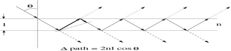
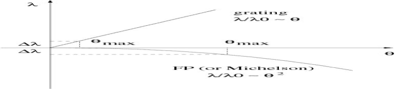
Figure 12: Basic concept of etalon-interference (left), and F-P versus grating spectral resolution as a function of angular aperture, $\theta$ (right).

1 Basic concepts and Field-Widening

Etalons (high-precision, flat glass plates) are parallel-spaced by some distance $l$, filled with gas of refractive index $n$, and coated to have high reflectivity. Light incident at some angle, $\theta$, produces internal reflections, with transmission when the added path ($\Delta{\rm path}=2\ n\ l\ cos\ \theta$) between reflections yields positive interference (left panel, Figure 1.12). The ratio of transmitted to incident intensity, $I_{t}/I_{i}$, is given approximately by an Airy function with peaks ($I_{t}=I_{i}$) when $\Delta{\rm path}=m\lambda$, where $m$ is the order. Given the geometry, this yields an angular dependence to the transmitted wavelength: $\lambda=(2\ n\ l\ /\ m)\ cos\ \theta$. This can be compared to the grating equation (Littrow configurations for simplicity), where $\lambda=2\ n\ \Lambda_{g}\ /\ m\ sin\ \theta$. At small angles, this means that the instrument entrance aperture can be larger in angle for a F-P compared to a grating spectrograph for the same $\delta\lambda$, as illustrated in the right panel of Figure 1.12. In other words, a F-P system is field-widened for the same spectral resolution (see also Roesler 1974 and Thorne 1988).

The central wavelength of the F-P is controlled via tuning the gap ($l$) or pressure (index $n$). The free spectral range is given by the spacing between Airy-function peaks in wavelength: $Q=1\ /\ 2\ n\ l\ cos\ \theta$. Order-blocking filters are needed to suppress other orders. Double etalons suppress the Lorentian wings in the Airy-function. The resolution, which is the full-width at half-maximum of the Airy formula peak, is given by: $R=\lambda/\delta\lambda=2\ n\ l\ \cos\theta\ N_{\Re}/\lambda=m\ N_{\Re}$, where $N_{\Re}$ is the reflective finesse defined as $N_{\Re}=\pi\Re^{1/2}/(1-\Re)$, and $\Re$ is the reflectivity. The finesse is equivalent to roughly the number of back and forth reflections, and gives the number of resolution elements within the free spectral range of the system; a typical value is $\sim$30 (see Tanaka et al. 1985 for a more detailed discussion). This implies that the spectral resolution, $R$, is roughly the total path difference divided by the wavelength. High spectral resolution requires high finesse or high order, with the gap size tuned for the desired wavelength. This also achieves high contrast between the maximum and minimum transmittance between orders: $I_{max}/I_{min}=(1+\Re)^{2}/(1-\Re)^{2}=1+\frac{4N_{\Re}^{2}}{\pi^{2}}$. Herbst & Beckwidth (1988) provide a nice illustration of these quantities.

2 F-P Monochromators

F-P’s are conventionally thought of as being used with collimated beams (Bland & Tully 1989 present a review a mini-review of such instruments from that era). In this case, there is the classic radial wavelength dependence in the image plane. At low spectral resolution the band-pass can be made nearly constant over a large field of view (Jones et al. 2002), as follows.

One way to characterize an etalon is by the size of its “bull’s eye,” or Jacquinot spot (Jacquinot 1954). The bull’s eye refers to the physical angle $\theta$ such that $\lambda_{0}/|\lambda_{0}-\lambda_{\theta}|<R$, and is given by $\theta_{max}=\cos^{-1}(1-1/R)\sim\sqrt{2/R}$. This quantity is independent of the telescope, and is a property of the etalon. By coupling to a telescope, it is possible to modify the angular scale ($\alpha$) sampled on the sky by the bull’s eye. Since $A\times\Omega$ is conserved, $\alpha=\theta D_{e}/D_{T}$, where $D_{e}$ is the etalon diameter and $D_{T}$ the telescope diameter.

F-P’s can, however, be used in converging (or diverging) beams, even near a focus (Bland-Hawthorn et al. 2001). Some examples include the optical F-P on the CFHT 3.6m, when used with the AO Bonnette (AOB) and the future F2T2, an near-infrared double-etalon system for FLAMINGOS-2 (Gemini 8m; Scott et al. 2006, Eikenberry et al. 2004a). Image information is preserved by sampling the beam at a down-stream focus, but the spectral resolution is lowered (for a given finesse) at any spatial location because each field angle on the sky is mapped into a range of physical angles through the etalon. The degradation is not particularly severe for lower-finesse etalons or very slow beams. The FLAMINGOS-2 multi-conjugate adapative optics (MCAO) focus for F2T2 is f/30, and the AOB F-P beam is f/40. If the total angular field of view is much smaller than the beam angle, or the focus is made telecentric, the band-pass is constant across field angles on the sky, and the system forms a highly uniform tunable filter. The AOB optics are not telecentric; this produces a radial degradation in the resolution.

3 F-P Spectrometers

Alternatively, the full spectral information can be extracted at the loss of the spatial information by placing the etalons at or near a telecentric focus and sampling the pupil in a collimated beam. The Wisconsin H$\alpha$ Mapper (WHAM; Reynolds et al. 1998) is the only astronomical example of this type of instrument. In this instance, the light is collimated after it passes through the etalons, never refocused, and a detector is placed at the pupil formed by the collimator. Field position on the detector contains spectral information: each radius corresponds to a different wavelength. This is similar to the monochromator application, except in this case each radial location on the detector has a superposition from all spatial locations on the sky within the instrument entrance aperture.

4 3D F-P Spectrophotometers

Grating-Dispersed FPI

Arguably the most interesting F-P monochromator mode is to eliminate the order-blocking filters, and grating-disperse the output beam to separate the orders onto the detector to increase the spectral multiplex. See, for example, le Coarer et al.’s (1995) description of PYTHEAS. Baldry et al. (2000) work out a particularly compelling case for a cross-dispersed echelle system. The gain in spectral multiplex does not necessarily cost spatial multiplex. In practice, some F-P’s are in spectrographs where they under-fill the detector and usable field in the image plane (e.g., RSS and F2T2). If the dispersion is significantly greater than the etalon resolution, then in addition to spectral multiplex, this mode adds band-limited slitless spectroscopy in each F-P order.

Pupil-Imaging FPI

The above discussion frames the notion that detection down-stream of an etalon at the pupil of a collimated beam provides spectral information but no spatial information, while detection at a focal surface provides the complement. A simple ray-trace shows that between these two locations spectral and spatial information are mixed. By using pupil imaging at the system input via a lenslet array (§1.2.9), detection at an intermediate surface in a converging beam can separate spatial and spectral information. Although this has never been done, in principle this could balance spatial and spectral multiplex and allow for true 3D spectroscopy in future, field-widened instruments.

5 Sky Stability

Because spectral channels are not observed simultaneously in monochromatic modes, atmospheric changes must be calibrated (see, for example, Atherton et al. 1982 in the context of TAURUS). Field stars may suffice if they are sufficiently featureless over the scanned wavelength range. Built-in calibration is desirable, which can be achieved, for example, via a dichroic feeding a monitoring camera. This capability is designed for new generation of instruments (e.g., ARIES, T. Williams, private communication).

6 Examples of Instruments

Two extremes in F-P instrumentation are highlighted by the RSS imaging F-P (Williams et al. 2002) and the WHAM non-imaging F-P. Both have 150 mm etalons, but the RSS system is coupled to a 9.2 m telescope with an 8 arcmin field of view, 0.2 arcsec sampling and spectral resolutions of 500, 1250, 5000, and 12,500. In contrast, WHAM is coupled to a 0.6m telescope, with a 1 deg field of view and angular resolution, spectral resolution of $R=25000$, and spectral coverage of about 166 resolution elements for one spatial element.

There are a large number of existing F-P monochromators (a.k.a., tunable filters), indicated even by the following incomplete list. Optical systems include, but are not limited to: PUMA (OAN-SPM 2.1m, Rosado et al. 1995), RFP (CTIO 1m and 4m; e.g., Sluit & Williams 2006), CIGALE (ESO 3.6m and OHP 1.9m; Boulesteix et al. 1984), FaNTOmM (OMM 1.6m, OHP 1.9m, and CFHT 3.6m; Hernandez et al. 2003), Goddard F-P (APO 3.5m; Gelderman et al. 1995), SCORPIO F-P (SAO 6m, Afanasiev & Moiseev 2005), IMACS F-P (Magellan 6.5m; Dressler et al. 2006), as well as the above-mentioned CFHT F-P etalons which can be used with the AOB as well as the MOS and SIS systems. The most widely cited system is TTF/TAURUS-II (AAT 3.9m, WHT 4.2m; Gordon et al. 2000 and references therein). Existing infrared instruments include NIC-FPS (Arc 3.5m; Hearty et al. 2004), GriF (CFHT 3.6m; Clenet et al. 2002), PUMILA (OAN-SPM 2.1m, Rosado et al. 1998), UFTI (UKIRT 3.8m, Roche et al. 2003) and NACO (VLT 8m; Hartung et al. 2004, Iserlohe et al. 2004). GriF, NACO, and F2T2 are AO-fed. By virtue of their use in collimated beams, many of the F-P systems are designed to be transportable between instruments (i.e., spectrographs or focal-reducers) and telescopes. Future instruments include the optical OSIRIS (GTC 10.4m) and near-infrared FGS-TF (JWST 6.5m; Davila et al. 2004) and F2T2 (above). These systems span a wide range of wavelength, spectral, and spatial resolution. One attribute they have in common is a spectral multiplex of unity.

4 Interferometry-II: Spatial-Heterodyne Spectroscopy

A spatial-heterodyne spectrometer (SHS) is a Michelson interferometer with gratings replacing the mirrors. The principles of operation are described and illustrated by Harlander et al. (1992) – a paper well-worth careful study. Briefly, each grating diffracts light at wavelength-dependent angles. Because of the 90-degree fold between the two beams, the wavefronts at a given wavelength are tilted with respect to each other after beam recombination. This tilting produces a sinusoidal interference pattern with a frequency dependent on the tilt angle. The degree of tilt is a function of wavelength, simply due to the grating diffraction, and hence the interference pattern frequency records the wavelength information.

It is easiest to conceptualize this in terms of two identical gratings (as illustrated by Harlander et al. in their Figures 2 and 3), but in principle the gratings do not need to be the same. Wavefronts produce interference patterns with frequencies set by wavelength, with the central wavelength producing no interference. Hence the signal is heterodyned about the frequency of the central wavelength. Resolution is set by the grating aperture diameter because this sets the wavelength (i.e., angular tilt) which minimally departs from the central wavelength which can produce the first (lowest) frequency for interference. Bandwidth is set by the length of the detector, i.e., how many frequencies can be sampled depends on the number of pixels.

The advantage of an SHS over a Michelson is that no stepping is required to gain the full spectral information, but the field of view is reduced. The SHS can be fed with a long-slit or lenslet array, although with the latter a band-limiting filter is needed (as with a conventional dispersed spectrograph). Like with a Michelson, however, field-widening is possible via prisms. In the SHS application, the prisms give gratings the geometric appearance of being more perpendicular to the optical axis, and hence larger field angles are mapped within the beam deviation producing the lowest-order interference fringe. Cross-dispersion is possible (by tilting one of the gratings about the optical axis), but the same fundamental limits apply concerning 3D information formatted into a 2D detector!

One of the problems with the standard Michelson or SHS interferometer is that their geometry throws out half the light right from the start. Non-lossy geometries are possible. Harlander et al. (1992) give an example of working off-axis on the collimating mirror (see their Figure 5). This is a perfect application for holographic gratings. Transmission-grating geometries would eliminate the need to go off-axis and probably allow for larger field. Another approach is a Mach-Zender style interferometer (Douglas 1990). The latter requires twice the detector real-estate for the same number of spectral resolution elements.

The primary advantage of an SHS is that it allows for very high spectral resolution for a given solid angle relative to a conventional, grating-dispersed spectrograph. The SHS is field-widened like a F-P. This means the SHS can be built for low cost even on large telescopes because the optics are small.

However, because the signal is in the form of an interferogram, there is what is known as the “multiplex disadvantage.” This can be expressed as the $S/N$ performance of the SHS relative to a grating spectrograph: $S/N_{SHS}=S/N_{GS}(f/2)^{1/2}(S_{SHS}/S_{GS})^{1/2}$, where $S/N_{SHS}$ and $S/N_{GS}$ are the signal to noise in SHS and grating spectrometer, respectively, $S_{SHS}$ and $S_{GS}$ are the total photon signal, respectively, and $f$ is the fraction of total signal in a given spectral channel ($f<1$, and decreases with bandwidth). In words, this means that an SHS looses competitiveness with grating-dispersed spectrographs when the band-pass is large. This has implications for design and use. Clearly one must make $S_{SHS}$ and $f$ as large as possible. The small, compact optics of a SHS system lend itself to efficiency optimization. To make $f$ as large as possible, one must choose a small band-width (but more than a Fabry-Perot monochromator!) and remove OH lines via pre-filtering, or by selecting band-passes between them. Returning to Figure 1, SHS is between a F-P monochromator and other IFS methods, and therefore will have application to a broad range of science programs that seek high spectral resolution over a limited band-pass with good spatial coverage.

5 Summary of Existing Instruments

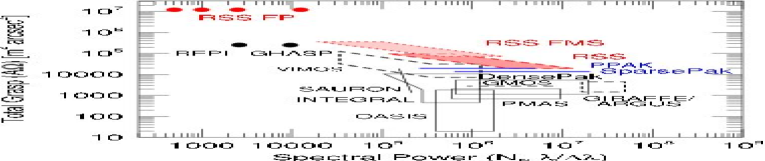
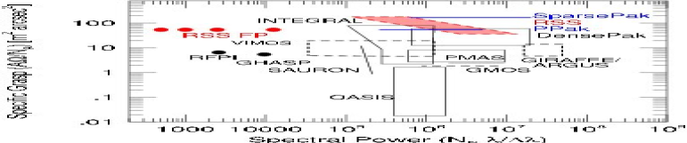
Figure 13: Total and Specific Grasp versus Spectral Power for a range of instruments on 4m- and 10m-class telescopes (solid and dashed lines, respectively) partially updated from Bershady et al. (2005). See text for comments on instrument efficiency.

Here we explore the sampled parameter space in spatial versus spectral information, as well as coverage versus resolution, starting with grasp and spectral power (Figure 1.13). Recall that because reliable, consistent measurements of efficiency are unavailable for most instruments, we use grasp instead of etendue (warning: we really want etendue). Note, however, that there is a factor of 6 range in the known efficiencies of instruments tabulated in this Chapter. Further note that there are two ways of viewing the specific grasp. From the perspective of staying photon-limited at high spectral resolution, high specific grasp is important. The “flip side” is that low specific grasp implies high angular resolution.

Figure 1.14 shows that spatial resolution is higher in NIR instruments, while spectral resolution is higher in optical instruments. Fiber IFUs have the largest specific grasp – reflected in the bifurcation seen in spatial resolution, i.e., fiber-fed instruments have large footprints per element ($d\Omega$). There is a trend of decreasing specific grasp going from fiber+lenslet, lenslet, and finally to slicers. ESI has unusually large $A\ \times\ d\Omega$ for a slicer; RSS in FMS mode has the highest specific grasp overall.

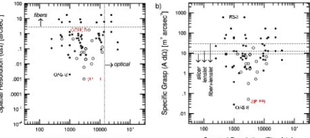
Figure 14: Spatial resolution (a) and specific grasp (b) versus spectral power for all instruments in Tables 1-4, highlighting differences between optical (filled symbols) and NIR (open symbols), as well as between different coupling methods (labeled).

Figure 1.14 and 1.15 together show that optical and near-infrared instruments trade spatial resolution for grasp; there are no high-grasp NIR instruments; the highest spectral power instruments are optical. Optical and near-infrared instruments sample comparable total information, with optical instruments sampling a broader range of trades between spatial versus spectral information. Older NIR instruments clearly suffer from being detector-size limited. IMACS-IFU stands out as having significantly larger number of total information elements, $N_{R}\ \times\ N_{\Omega}$, and in this sense is on-par with future-generation instruments.

6 The Extended-source Domain

One area of extra-galactic science is clearly under-sampled by existing instrumentation, namely high spectral-resolution yet low surface-brightness 3D spectroscopy of extended sources. The scientific impetus is for detailed nebular studies (ionization, density, metallicity, abundances) of not only compact HII regions, but to extend such study to the diffuse ionized gas. Likewise, a significant fraction of the stellar light in galaxies is in extended distributions at low surface-brightness, i.e., below the night-sky background. The kinematic and chemical properties of these stars is largely unknown outside of resolved populations in the Local Group. Stellar kinematics of galaxies on spatially-resolved scales are required to dissect the mass distribution and detailed dynamics of disk, bulge, and halo components. This information is effectively the Rosetta Stone for deciphering how galaxies have assembled.

One concern with most existing IFU spectrographs is their focus on very fine spatial sampling. Referring back to Figure 1.4, on telescopes as small as only 10m (!), this severely limits the spectral resolution that can be achieved at sub-arcsec sampling in the photon-limited regime. For example, FLAMES/GIRAFFE is unusual in its high spectral resolutions of 10-40,000. Each IFU unit is a $2\times 3$ arcsec of 20 rectangular microlenses sampling only $0.52\times 0.52$ arcsec; this is equivalent to a 1 arcsec fiber on 3.5m telescope. The instrument is very close to the photon-detector–limited divide. The IMACS-IFU should be in a similar domain at its high spectral-resolution limit.

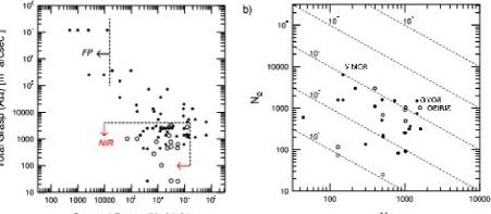
Figure 15: Total grasp versus spectral power (a) and the number of spatial ($N_{\Omega}$) versus spectral ($N_{R}$) resolution elements (b) for all instruments in Tables 1-4, highlighting differences between optical (filled symbols) and NIR (open symbols). Dashed lines are at constant (labeled) total information ($N_{R}\ \times\ N_{\Omega}$).

There is no question FLAMES/GIRAFFE has proven spectacular for emission-line work, particular if line-emission is clumpy and unresolved, e.g., ionized-gas kinematics of distant galaxies (Flores et al. 2004). The need for high angular resolution in the distant-galaxy kinematic game is paramount. Even with $\sim$0.5 arcsec resolution, HST images are needed to super-resolve the IFU data (Flores et al. 2004). It will be difficult, however, to use this same facility to study diffuse gas or the stellar continuum in resolved sources. Furthermore, resolved structures at high redshift are all at apparently low surface-brightness because of cosmological dimming. To stay photon-limited, observing in the low-surface-brightness regime requires either lower spectral resolution, larger apertures ($d\Omega$), or larger telescopes. Will this be addressed by future instrumentation?

7 Future Instruments

The next generation of instruments will compete on both space-based platforms such as the JWST, and on ground-based telescopes reaching 30m or larger in diameter. Why build these bigger telescopes? The argument of simply collecting more photons is compelling but not sufficient. New facilities, which come at increasingly greater cost, must yield gains above the linear increase in area. Such “windfalls” may include over-coming detector-noise, the diffraction-limit (at long wavelengths), backgrounds (in the case of space-based platforms), or critical combinations thereof.

A discussion of backgrounds and the relative merits and niches of 8m-class space-based telescope such as JWST, and large 30m-class ground-based telescopes was vetted in the early planning stages of what was once known as “MAXimum Aperture Telescopes,” or MAXAT. Gillett & Mountain (1998) pointed out that a cooled space-craft has significantly lower background in the infrared compared to the ground – even at high spectral resolution. This contrast is dramatic for $\lambda>2.5\mu m$, i.e., in the thermal-IR. However, they calculated that above $R\sim 1000$, 8m-class space-telescopes are detector-limited at any wavelength, assuming 0.05 arcsec apertures, a generous system throughput, and realistic detectors. They constructed a competitiveness criteria which assumed diffraction-limited performance for stellar imaging or spectroscopy. Compared to JWST, they concluded ground-based telescopes can be competitive at $\lambda<2.5\mu m$ for imaging if $D_{T}>20m$, and for diffraction-limited spectroscopy at $R>1000$ for $D_{T}>8m$ at any wavelength. These considerations have been influential on the planning and design of future-generation instruments in the era of JWST.

1 Ground-based Instruments on 10m Telescopes

Given rapid growth in 3D spectroscopy, we expect many new and retro-fitted systems in the coming years. We sketch three instruments – MUSE, VIRUS, and KMOS – because they highlight the common themes of object and instrument multiplexing. (US scientists will note two of these systems are on the VLT.) Object multiplexing is a departure for 3D instrumentation; instrument multiplexing is a departure overall. The basic parameters of these 3 instruments are summarized in Tables 1,3.

Both MUSE and VIRUS offer unprecedented spatial sampling. MUSE provides a truly integral 1 arcmin² area, sampled at the 0.2 arcsec scale, accomplished via image slicing (AIS-type). The most significant portions of the system are the slicers, which must perform well (with little scattered light) in the optical, and the field-partitioning between a bank of 24 identical spectrographs. In comparison, the individual spectrographs are modest, albeit high-efficiency, articulated VPH-grating systems.

VIRUS uses the same notion of a replicated spectrograph unit (also articulated VPH-grating systems), but in this case fed by bare fibers at a much coarser scale ($25\times$ larger $d\Omega$). The field sampling is sparse, and hence this instrument follows directly in the path of bare-fiber IFUs. What stands out in the VIRUS design is the “Ultra-cheap” notion of the spectrograph unit, i.e., by building many, replicated units, costs are lowered by economies of scale. Such a demonstration has important implications for future large-telescope instrument design (how large must the replication scale be to manifest significant economy?). If the full replication of 132 spectrographs is accomplished, this will be by far the widest-field (largest grasp) IFU in existence, likely for years to come. To achieve the VIRUS-132 goal requires an all new, wide-field prime-focus spherical-aberration corrector yielding a 16 arcmin science-grade field for the HET – a significant opto-mechanical challenge in itself.

MUSE, in contrast to VIRUS, has 9$\times$ less total grasp, but almost 3$\times$ more spatial elements ($N_{\Omega}$). In other words, both stand out as remarkable in spatial sampling in their own way. The differences in spatial resolution versus coverage between MUSE and VIRUS lies in their respective science themes. VIRUS is designed as a precision-cosmology engine to measure the baryon oscillations by detecting $z\sim 3$ Ly$\alpha$-emitters, and using their distribution as a density tracer. These sources are relatively rare (in surface-density to a given detected flux), although the exact flux-density relation is still uncertain. Rather low spectral resolution ($R<1000$) is needed, since only line-identification (in the blue where backgrounds are low) and redshifts are required.

MUSE, in contrast, is designed to probe the detailed internal properties (dynamics, stellar populations) of galaxy populations over a wide range in redshift and in a representative cosmological volume. The aim of this instrument is essentially to enable spectroscopic versions of many “Hubble Deep Fields,” each with sufficient spectral and spatial information to extract kinematics and line-diagnostics of many thousands of $z<1$ galaxies.

KMOS has much the same science goals of MUSE, with the key distinction of pushing to higher redshifts by using the NIR to capture the optical rest-frame. By pushing to higher redshift to gain temporal leverage on the galaxy formation and evolution process, the source-distribution becomes apparently fainter, and the NIR backgrounds are higher. Consequently, on the same size telescope, one is forced to look at intrinsically more luminous and hence rarer objects. Therefore, the KMOS design moves away from the notion of a monolithic integral-field, to a 24-probe system in a large, 7.5 arcmin diameter patrol field. Each probe spans a $2.8\times 2.8$ arcsec area sampled at $0.2\times 0.2$ arcsec. While a multi-IFU instrument already exists (again on the VLT) in the optical with FLAMES/GIRAFFE, the extension to the NIR using slicers with twice the number of probes will be a significant technical achievement.

What is missing from this suite of remarkable instruments is a design which pushes forward a significant increase in spectral sampling (spectral power) or specific grasp. For example, none of these instruments offers over $R=4000$ and $N_{R}=2000$. This means, for example, that advances in the study of low surface-brightness, dynamically cold ($\sigma<80$ km/s) systems or nebular regions will require additional instrument innovation.

2 Ground-based Instruments on 30-50m Class Telescopes

Table 5: Future TMT Integral Field Instruments

Instrument	Coupling	DT	$\Omega$	d$\Omega$	NΩ	$\Delta\lambda/\lambda$	R	NR	$\epsilon$
		(m)	(arcsec2)
IRMOS	slicer	30.	40.	0.01	4000	0.25	2000	500	$\cdots$
IRMOS	slicer	30.	40.	0.01	4000	0.25	10000	2500	$\cdots$
IRIS	slicer	30.	0.26	1.6e-5	16384	0.05	4000	200	$\cdots$
IRIS	slicer	30.	1.33	8.1e-5	16384	0.05	4000	200	$\cdots$
IRIS	slicer	30.	7.93	4.8e-4	16384	0.05	4000	200	$\cdots$
IRIS	slicer	30.	41.0	2.4e-4	16384	0.05	4000	200	$\cdots$
WFOS	fiber+lens	30.	810.	0.56	1440	1.37	5000	6850	0.3

We summarize some of the specific exmaples of TMT 3D-spectroscopic instrumentation in Table 5, based on D. Crampton’s overview (Ringberg 2005; Crampton & Simard 2006). TMT instrument design is largely driven by AO capabilities, where the salient point is that there are many “flavors” of AO, with associated levels of difficulty and risk (inversely proportional to their performance in either image quality, field of view, or both). The IFU-capable TMT instruments include, in order of decreasing AO requirements: (i) IRMOS, a NIR multi-object integral-field spectrograph fed by the multi-object adaptive object system (MOAO), capable of 20 positional, 5 arcsec compensated patches within a 5 arcmin patrol field; (ii) IRIS, a NIR imager and integral field spectrograph working at the diffraction limit, fed by the narrow-field facility AO system (NFIRAOS); and (iii) WFOS, an optical, wide-field, seeing-limited spectrograph with potential for a modest-grasp IFU with good spectral power and spectral resolution ($R<6000$).

With the exception of WFOS, instrument design is driven by AO considerations because of the enormous physical size of the image (which scales with mirror diameter for a constant f-ratio). WFOS is necessarily a monster. The AO-driven focus is suitable for scientific studies of un- or under-resolved sources (stars, planets, sub-kpc scales in distant galaxies), and excellent science-cases have been developed. Of this excellence there is no doubt. Of concern is that once wedded to the notion of a very large telescope with no clear path to building affordable, comparably-monstrous instruments, one is forced down a path, ab initio, of considering only science enabled by high-angular resolution. It is not surprising to note that WFOS – the one non-AO corrected instrument – stands out as also the one TMT instrument concept that breaks into the high specific-grasp domain at modest spectral-resolution domain (Figure 1.16). Indeed, as seen in Figure 1.17, WFOS breaks new ground in terms of its total grasp at the highest spectral power of any existing instrument (save ESI). To optimize low-surface-brightness studies, other paths will need to be forged to push to higher spectral power and resolution at comparably high grasp.

These same trends are also being played out for instrument design for ELT (e.g., Eisenhauer et al. 2000, Russell et al. 2004). We’ve focused on TMT because of the more mature stage of this telescope’s planning. No doubt ELT’s complement of instruments will open up exciting new capabilities, as demonstrated by the superb, forefront instrumentation on the VLT. The TMT instrumentation program, like that of the European ELT, is evolving rapidly. What is presented here is a snapshot circa late 2005.

3 Space-based Instruments

Table 6: Future Space-Based Integral Field Instruments

Instrument	Coupling	Tel.	DT	$\Omega$	d$\Omega$	NΩ	$\Delta\lambda/\lambda$	R	NR	$\epsilon$
			(m)	(arcsec2)
FGS-TF	FP	JWST	6.5	38088.	0.018	2.10e7	0.01	100	1	$\cdots$
NIRSpec	AIS	JWST	6.5	9.	0.0056	1600	0.34	3000	1024	$\cdots$
MIRI	AIS	JWST	6.5	51.8	0.30	173	1.48	2800.	4096	$\cdots$
SNAP-IFU	AIS	SNAP	2.	9.0	0.022	400	1.95	100	195	0.44

We summarize the planned 3D-spectroscopic instruments for JWST and SNAP (Super Nova Acceleration Probe; Aldering et al. 2002) in Table 1.6. (There are other missions, which include IFUs, also in the planning stages.) On JWST, in remarkable constrast to HST, three of the four instruments have 3D spectroscopic modes in the near- and mid-infrared: (i) FGS-TF (of which F2T2 is the ground-based analogue) delivers a $2.3\times 2.3$ arcmin field at $R\sim 100$, with two cameras covering 1.2 to 4.8 $\mu$m. (ii) NIRSpec (Prieto et al. 2004) has a $3\times 3$ arcsec IFU using and AIS with 40 $3\times 0.075$ arcsec slices, covering 0.8-5 $\mu$m at $R=3000$. (iii) MIRI (Wright et al. 2004) has 4 simultaneous image-slicers at $R\sim 3000$ feeding 4 wave-bands between 5-28 $\mu$m. Each samples $4.6\times 5.5$ arcsec (increasing by a factor of two between bluest and reddest channel) with an 0.37 arcsec slit-width (changing by a factor of 4 between bluest and reddest channel). Quoted numbers represent mean values over all channels.

The SNAP IFU (Ealet et al. 2003) is designed to identify SNe type out to $z\sim 1.7$. As such, it is unique in being dual optical-NIR systems (0.35-1.7 microns), with a $3\times 3$ field using AIS, but very low spectral resolution ($R=100$). With its very high expected efficiency, coadded data-sets should yield superb, spatially resolved spectrophotometry of galaxies on 1-2 kpc scales.

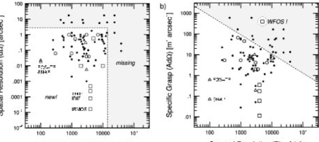
Figure 16: Spatial resolution (a) and specific grasp (b) versus spectral power including future instruments in Tables 5 and 6: existing (filled circles), future ground-based 10m-class telescope (open circles), future TMT (open squares), and future space-based (open triangles).

Overall, future space-based capabilities can be characterized as having $3\times 3$ arcsec fields mapped with AIS-technology with 0.15 arcsec sampling – lower spatial resolution than TMT. Spectral resolution is in the $100<R<3000$ range, again lower than TMT. This is consistent with their being competitive in performance relative to TMT-class instruments, given Gillett & Mountain’s (1998) argument. However, there are no large-grasp systems that take full advantage of the low backgrounds of space. There are no high- or even medium-resolution spectrographs to couple, competitively, to such large angular apertures. Nonetheless, barring past fiascos, the space-based missions offer the guarantee of superlative image quality and low backgrounds extending into the mid-IR, while ground-based observatories face the intense challenge of developing advanced AO systems.

4 Summary of Future Instruments

While Figure 1.16 shows some of the areas not accessed by currently planned future instrumentation, at the same time clearly great strides are planned for accessing new domains in spatial resolution – from the ground. This is encouraging because only with the largest apertures can we stay photon-limited at moderate spectral resolution. JWST instruments present the unique ability to work at more modest spectral resolution and still remain source-photon limited. Space-based instruments, overall, will also provide the most-stable and best-characterized PSFs – a premium for high angular-resolution spectrophotometry.

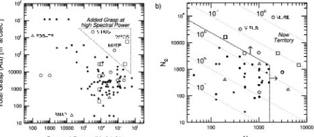
Figure 17: Total grasp versus spectral power (a) and the number of spatial ($N_{\Omega}$) versus spectral ($N_{R}$) resolution element (b) including future instruments in Tables 5 and 6: symbols as in previous figure.

Figure 1.17 reveals where new instruments open up new territory – both in added grasp at high spectral power, and simply in more resolution elements ($N_{R}\ \times\ N_{\Omega}$). Of particular note is the thrust toward instruments with many thousands of spectral resolution elements. These gains are seen for both ground- and spaced-based instruments, on both 10m- and 30m-class telescopes.

These gains are made with conceptually conventional grating-dispersed systems or F-P monochromators. Clearly there is opportunity for less-conventional field-widened instruments (such as the interferometric concepts discussed above), which can amplify both grasp and spectral power or spectral resolution. Given the relative novelity of these approaches, they present higher risk, but potentially higher return, and are best suited for ground-based development.

Acknowledgements. We would like to thank the IAC and Winter School organizers, the University of Toronto Department of Astronomy & Astrophysics for their gracious hospitality during a sabbatical year where this work was done, and the NSF for their financial support of this research (AST-0307417 and AST-0607516).

References

- [1]
- [2]
- [3] Afanasiev, V.L, Dodonov, S.N., Sil’chenko, O.K., Vlasyuk, V.V. 1990, SAO preprint N54
- [4] Afanasiev V. L., Moiseev, A.V. 2005, Astr. Lett., 31, 193
- [5] Aldering, G. et al. 2002, Proc. SPIE, 4835, 146
- [6] Alighieri, S.S. 2005, in the Proceedings of the ESO Workshop on Science Perspectives for 3D Spectroscopy, (Garching, Germany)
- [7] Allende Prieto, C., Majewski, S. R., Schiavon, R. et al. 2008, AN, 329, 1081
- [8] Allington-Smith, J., Content, R. 1998, PASP, 110, 1216
- [9] Allington-Smith, J., et al. 2002, PASP, 114, 892
- [10] Allington-Smith, J., et al. 2004, Proc. SPIE, 5492, 701
- [11] Arribas, S., Mediavilla, E., Rasilla, J.L. 1991, ApJ, 369, 260
- [12] Arribas, S., et al. 1998, ASPCS, 152, 149
- [13] Atherton, P.D., Taylor, K., Pike, C.D., Harmer, C.F.W., Parker, N.M., Hook, R.N. 1982, 201, 661
- [14] Avila, G., Guinouard, I., Jocou, L., Guillon, F., Balsamo, F. 2003, Proc. SPIE, 4841, 997
- [15] Bacon, R., et al. 2001, MNRAS, 326, 23
- [16] Bacon, R., et al. 2004, Proc. SPIE, 5492, 1145
- [17] Baldry, I.K., Bland-Hawthorn, J. 2000, 112, 1112
- [18] Baldry, I.K., Bland-Hawthorn, J., Robertson, J.G. 2004, PASP, 116, 403
- [19] Barden, S.C., Wade, 1988, ASPCS, 3, 113
- [20] Barden, S.C., Elston, R., Armandroff, T., Pryor, C 1993, ASPCS, 37, 223
- [21] Barden, S.C., Sawyer, D.G., Honneycutt, R.K. 1998, Proc. SPIE, 3355, 892
- [22] Barden, S.C., Arns, J.A., Colburn, W.S., Williams, J.B 2000, PASP, 112, 809
- [23] Baranne, A. 1972, in ESO/CERN Conference on Auxiliary Instrumentation for Large Telecsopes, ed. S. Lautse & A. Reiz (Geneva), 227
- [24] Bershady, M.A., Andersen, D.R., Harker, J., Ramsey, L.W., Verheijenn, M.A.W. 2004, PASP, 116, 565
- [25] Bershady, M.A., Barden, S., Blanche, P.-A. et al. 2008, Proc. SPIE, 7014, 70140H-1
- [26] Bershady, M.A., Andersen, D.R., Verheijen, M.A.W., Westfall, K.B., Crawford, S. M., Swaters, R.A. 2005, ApJS, 156, 311
- [27] Blais-Ouellette, S., Guzman, D., Elgamil, A., Rallison, R. 2004, Proc. SPIE, 5494, 278
- [28] Blais-Ouellette, S., Daigle, O., Taylor, K. 2006, Proc. SPIE, 6269, 174
- [29] Bland, J., Tully, R.B. 1989, AJ, 98, 723
- [30] Bland-Hawthorn, J., van Breugel, W., Gillingham, P.R., and Baldry, I.K. 2001, ApJ, 563, 611
- [31] Bonnet, H. 2004, The ESO Messenger, (Vol: September), 17
- [32] Boulesteix, J., Georgelin, Y., Marcelin, M., Monnet, G. 1984, Proc. SPIE, 445, 37
- [33] Burgh, E.B., Nordsieck, K.H., Kobulnicky, H.A., Williams, T.B., O’Donoghue, D., Smith, M.P., Percival, J.W., 2003, Proc. SPIE, 4841, 1463
- [34] Burgh, E.B., Bershady, M. A., Nordsieck, K.H., Westfall, K. B. 2007, PASP, 119, 1069
- [35] Carrasco, E., Perry, I.R. 2004, MNRAS, 271, 1
- [36] Clenet, Y. et al. 2002, PASP, 114, 563
- [37] le Coarer, E., Bensammar, S., Comte, G., Gach, J.L., Georgelin, Y. 1995, A&A Supp., 111, 359
- [38] Crampton, D. & Simard, L. 2006, Proc. SPIE, 6269, 59
- [39] Davila, P. et al. 22004, Proc. SPIE, 5487, 611
- [40] Dopita, M.A., et al. 2004, Proc. SPIE, 5492, 262
- [41] Douglas, N.G., Butcher, H.R., Melis, & M.A. 1990, Ap&SS, 171, 307
- [42] Dressler, A., Hare, T., Bigelow, B.C., Osip, D.J. 2006, Proc. SPIE, 6269, 13
- [43] Ealet, A. et al. 2003, Proc. SPIE, 4850, 1169
- [44] Eikenberry, S. et al., 2004a, Proc. SPIE, 5492, 1196
- [45] Eikenberry, S. et al., 2004b, Proc. SPIE, 5492, 1264
- [46] Eisenhauer, F., Tecza, M., Thatte, N., Mengel, S., Hofmann, R., Genzel, R. 2000, Proceedings of the Backaskog Workshop on Extremely Large Telescopes, ed. T. Andersen, A. Ardeberg, R. Gilmozzi (Lund/ESO), 57, 292
- [47] Eisenhauer, F., et al. 2003, Proc. SPIE, 4841, 1548
- [48] Fabricant, D., et al. 1998, Proc. SPIE, 3355, 285
- [49] Fabricant, D., et al. 2005, PASP, 117, 1411
- [50] Flores, H., Peuch, M., Hammer, F., Garrido, O., Hernandez, O. A&A, 420, L31
- [51] Geake, J.E., Ring, J., Woolf, N.J. 1959, MNRAS, 119, 161
- [52] Gelderman, R., Woodgate, B.E., Brown, L.W. 1995, ASPC, 71, 89
- [53] Gillett, F., & Mountain, M. 1998, ASPC, 133, 42
- [54] Gordon, S., Koribalski, B., Houghton, S., Jones, K. 2000, MNRAS, 315, 248
- [55] Guerin, J., Felenbok, P. 1988, ASPCS, 3, 52
- [56] Hanuschik, R.W. 2003, A&A, 407, 1157
- [57] Harlander, J., Reynolds, R.J., Roseler, F.L. 1992, ApJ, 730
- [58] Hartung, M., Lidman, C., Ageorges, N., Marco, O., Kasper, M., Clenet, Y. 2004, Proc. SPIE, 5492, 1531
- [59] Haynes, R. et al. 1999, PASP, 111, 1451
- [60] Hearty, F. R. et al. 2004, Proc. SPIE, 5492, 1623
- [61] Henault, F. et al., 2004, Proc. SPIE, 5249, 134
- [62] Herbst, T.M., Beckwidth, S. 1988, PASP, 100, 635
- [63] Hernandez, O., Gach, J.-L., Carignan, C., Boulesteix, J. 2003, Proc. SPIE, 4841, 1472
- [64] Hill, G., et al. 2004, Proc. SPIE, 5492, 251
- [65] Iserlohe, C. et al. 2004, Proc. SPIE, 5492, 1123
- [66] Jacquinot, P. 1954, J. Opt. Soc. Am., 44, 761
- [67] Joncas, G. and Roy, J.R. 1984, PASP, 96, 263
- [68] Jones, D.H., Shopbell, P.L., Bland-Hawthorn, J. 2002, MNRAS, 329, 759
- [69] Kelz, A. et al. 2006, PASP, 118, 119
- [70] Kenworthy, M.A., Parry, I.R., Ennico, K.A. 1998, ASPCS, 152, 300
- [71] Kenworthy, M.A., Parry, I.R., Taylor, K. 2001, PASP, 113, 215
- [72] Kelson, D. 2003, PASP, 115, 688
- [73] Kobulnicky, H.A., Norsieck, K.H., Burgh, E.B., Smith, M.P., Percival, J.W., Williams, T.B., O’Donoghue, D. 2003, Proc. SPIE, 4841, 1634
- [74] Koo, D.C., Bershady, M.A., Wirth, G.D., Stanford, S.A., Majewski, S.R. 1994, ApJ, 427, L9
- [75] Larkin, J. et al. 2003, Proc. SPIE, 4841, 1600
- [76] Le Fevre, O., Crampton, D., Felenbok, P., Monnet, G. 1994, A&A, 282, 325
- [77] Le Fevre, O. et al. 2003, Proc. SPIE, 4841, 1671
- [78] Lissandrini, C., Cristiani, S., La Franca, F. 1994, PASP, 106, 1157
- [79] Lorenzetti, D., et al. 2003, Proc. SPIE, 4841, 94
- [80] Maihara, T. et al. 1993, PASP, 105, 940
- [81] McDermid, R., Bacon, R., Adam, G., Benn, C. and Cappellari, M. 2004, Proc. SPIE, 5492, 822
- [82] McGregor, P.J., et al. 2003, Proc. SPIE, 4841, 1581
- [83] Murphy, T.W., Matthews, K., Soifer, B.T. 1999, PASP, 111, 1176
- [84] Nelson, G.W. 1988, ASPCS, 3, 2
- [85] Oliveira, A.C., de Oliveira, L.S., dos Santos, J.B. 2005, MNRAS, 356, 1079
- [86] Parry, I. et al. 2004, Proc. SPIE, 5492, 1135
- [87] Prieto, E., Ferruit, P., Cuby, J.-G., Blanc, P.-E., Le Fevre, O. 2004, Proc. SPIE, 5487, 777
- [88] Rallison, R.D., Schicker, S.R. 1992, Proc. SPIE, 1667, 266
- [89] Ramsay Howat, S.K., Todd S., Wells, M., Hastings, P. 2006, New Astronomy Reviews, 50, 3513
- [90] Ramsey, L.W. 1988, ASPCS, 3, 26
- [91] Ren, D. and Allington-Smith, J. 2002, PASP, 114, 866
- [92] Reynolds, R.J., Tufte, S.L., Haffner, L.M., Jaehnig, K., Percival, J.W. 1998, PASA, 15, 14
- [93] Roche, P. F., et al. 2003, SPIE, 4841, 901
- [94] Roesler, F.L. 1974, Methods in Experimental Physics, 12A, (Academic Press: San Diego), Chapter 12
- [95] Rosado, M. et al. 1995, RMxAC, 3, 263
- [96] Rosado, M. et al. 1998, SPIE, 3354, 1111
- [97] Roth, M.M., et al. 2005, PASP, 117, 620
- [98] Russell, A.P.G. et al. 2004, Proc. SPIE, 5492, 1796
- [99] Saunders, W. et al. 2004, Proc. SPIE, 5492, 389
- [100] Schroeder, D., 2000, Astronomical Optics, Academic Press (San Diego), 2nd Edition
- [101] Schmoll, J., Roth, M.M., Laux, U. 2003, PASP, 115, 854
- [102] Schmoll, J., Dodsworth, G.N., Content, R., Allington-Smith, J.R. 2004, Proc. SPIE, 5492, 624
- [103] Scott, A. et al. 2006, Proc. SPIE, 6269, 176
- [104] Sharples, R.M. et al. 2004, Proc. SPIE, 5492, 1179
- [105] Sheinis, A.I. et al. 2002, PASP, 114, 851
- [106] Sheinis, A.I. 2006, Proc SPIE (astro-ph/0606176)
- [107] Sluit, A.P.N., and Williams, T.B. 2006, AJ, 131, 2089
- [108] Tamura, N., Murray, G.J., Sharples, R.M., Robertson, D.J., Allington-Smith, J.R. 2005, Opt. Express, 13, 4125 (astro-ph/0509913)
- [109] Tanaka, M., Yamashita, T., Sato, S., Okuda, H. 1985, PASP, 97, 1020
- [110] Thatte, N. et al. 1994, Proc. SPIE, 2224, 279
- [111] Thatte, N. et al. 2000, ASPCS, 195, 206
- [112] Thorne, A.P. 1988, Spectrophysics, (Chapman & Hall: London)
- [113] Tull, R.G., MacQueen, P.J., Sneden, C., Lambert, D.L. 1995, PASP, 107, 251
- [114] Vaughan, A.H. 1967, ARAA, 5, 139
- [115] Verheijen, M.A.W. et al. 2004, Astron. Nachr., 325, 151
- [116] Viton, M., & Milliard, B. 2003, PASP, 115, 243
- [117] Williams, T.B., Nordsieck, K.H., Reynolds, R.J., Burgh, E.B. 2002, ASPC, 282, 441
- [118] Wright, G. et al. 2004, SPIE, 5487, 653
- [119] Wynne, C.G. 1991, MNRAS, 250, 796
- [120] Wynne, C.G., Worswick, S.P. 1989, MNRAS, 237, 239
- [121] Yee, H.K.C., Ellingson, E., Carlberg, R.G. 1996, ApJS, 102, 269