Single- and multi-peak solitons in two-component models of metamaterials and photonic crystals

Abstract

We report results of the study of solitons in a system of two nonlinear-Schrödinger (NLS) equations coupled by the XPM interaction, which models the co-propagation of two waves in metamaterials (MMs). The same model applies to photonic crystals (PCs), as well as to ordinary optical fibers, close to the zero-dispersion point. A peculiarity of the system is a small positive or negative value of the relative group-velocity dispersion (GVD) coefficient in one equation, assuming that the dispersion is anomalous in the other. In contrast to earlier studied systems of nonlinearly coupled NLS equations with equal GVD coefficients, which generate only simple single-peak solitons, the present model gives rise to families of solitons with complex shapes, which feature extended oscillatory tails and/or a double-peak structure at the center. Regions of existence are identified for single- and double-peak bimodal solitons, demonstrating a broad bistability in the system. Behind the existence border, they degenerate into single-component solutions. Direct simulations demonstrate stability of the solitons in the entire existence regions. Effects of the group-velocity mismatch (GVM) and optical loss are considered too. It is demonstrated that the solitons can be stabilized against the GVM by means of the respective “management” scheme. Under the action of the loss, complex shapes of the solitons degenerate into simple ones, but periodic compensation of the loss supports the complexity.

I Introduction and the model

Theoretical and experimental studies of various artificial optical media have recently drawn a great deal of interest, see, e.g., Refs. art and references therein. Among these, a well-known class is formed by metamaterials (MMs) based on the intrinsic periodic structures, built with subwavelength characteristic scales, that feature a combination of negative dielectric permittivity and magnetic permeability, and thus give rise to the negative refractive index Pendry . MMs promise a number of potential applications impossible in ordinary optical media, such as superlensing superlense ; Shalaev . MMs are also described as “left-handed” waveguides, as they were originally predicted as those where the wave vector of the electromagnetic wave is antiparallel to the usual right-handed cross product of the electric and magnetic fields Veselago . The intensive work has resulted in the creation of MMs featuring the negative refraction at optical frequencies Shalaev . Existing MMs are usually assembled as periodic arrays of metallic split-ring resonators, with various modifications of this basic setting.

Theoretical analysis of various nonlinear effects in models of MMs including cubic theory -Zhou or quadratic Scalora ; Haus terms has also drawn considerable attention. Some of these studies predict the existence of solitons in models of the MM type solitons . In particular, a theoretical model for the XPM (cross-phase-modulation)-mediated interaction of co-propagating waves, carried through the MM at different frequencies, is similar to the well-known two-wave model of ordinary media (where, in particular, it may give rise to the modulational instability in the case of the normal group-velocity dispersion (GVD) Agrawal , and to domain-wall patterns DW , in the same case). However, an essential peculiarity of the MM model is that the co-propagating waves may have widely different GVD coefficients, even with opposite signs, corresponding to normal and anomalous dispersion Zhou . Another type of artificially built optical media where this feature may be realized is represented by photonic crystals (PCs) and PC fibers PCF ; book . In fact, these possibilities illustrate the versatilely of artificial optical systems, which allow one to engineer required properties, that may often be made very unusual.

The main subject of the present work is constructing families of stable solitons within the framework of the system of XPM-coupled NLS (nonlinear-Schrödinger) equations describing the co-propagation of two waves with local amplitudes $u(z,\tau)$ and $v\left(z,\tau\right)$, carried by different frequencies:

$$iu_{z}+(1/2)u_{\tau\tau}+\left(|u|^{2}+2|v|^{2}\right)u = 0,$$ (1)

$$iv_{z}+icv_{\tau}+(1/2)D_{2}u_{\tau\tau}+\left(|v|^{2}+2|u|^{2}\right)v = 0.$$ (2)

Here $z$ and $\tau$ are, as usual, the propagation distance and reduced time, the GVD coefficient in Eq. (1) is normalized to be $D_{1}\equiv 1$ (which implies the anomalous sign of the GVD for wave $u$), $D_{2}$, that may have either sign, is the relative dispersion for the second wave ($D_{2}<0$ implies that wave $v$ propagates with normal GVD), $c$ is the walk-off parameter (alias the group-velocity mismatch, GVM, between the two carrier frequencies), which is an essential ingredient of the respective MM model SpecialTopics , and it is assumed that effective Kerr-nonlinearity coefficients are equal for both waves.

It is relevant to mention that the GVM between the fundamental-frequency and second-harmonic waves also plays an important in role in the MM model with the $\chi^{(2)}$ nonlinearity. An interesting feature of that system is that the phase locking of the second harmonic to the fundamental one, which is strongly affected by the GVM, may effectively impose the action of the negative refractive index on the second harmonic even in the situation when it directly affects only the fundamental frequency Haus .

Stationary solutions to Eqs. (1) and (2) with two independent wavenumbers of the components, $K_{u,v}$, are looked for as

$$\left\{u\left(z,\tau\right),v\left(z,\tau\right)\right\}=\exp\left(iK_{u,v}z\right)\left\{U(\tau),V(\tau)\right\}.$$ (3)

In the case of $c=0$, the stationary waveforms $U,V$ may be assumed real, obeying the equations following from the substitution of expressions (3) into Eqs. (1) and (2):

$$\begin{array}[]{c}(1/2)U^{\prime\prime}+\left(U^{2}+2V^{2}\right)U=K_{u}U,\\ \left(D_{2}/2\right)U^{\prime\prime}+\left(V^{2}+2U^{2}\right)V=K_{v}V.\end{array}$$ (4)

Equations (1) and (2) were recently derived in the context of MMs, neglecting the loss Zhou . In fact, the presence of strong losses is an inherent property of MMs loss , and, moreover, it has been rigorously proved that the negative refraction is not possible in a lossless medium necessary-loss . Nevertheless, schemes have been proposed to essentially compensate the MM loss, using the matched impedance Shalaev ; matched-impedance or various gain mechanisms gain . In any case, it makes sense to study solitons in conservative models of the MM type Zhou ; no-loss . In addition, the model based on Eqs. (1) and (2) may also be realized in PCs and PC fibers, where losses are present too, but as a less severe problem PCF . On the other hand, as concerns solitons, a relevant approach may be to include a lossy MM sample, along with an amplifier, as elements into an optical cavity, and predict cavity solitons possible in such a setting cavity .

As mentioned above, Eqs. (1) and (2) also apply to the description of the co-propagation of XPM-interacting waves in usual optical media, such as optical fibers Agrawal , although in that case most works have been dealing with the case of equal GVD coefficient, $D_{2}=1$. Nevertheless, the case of $D_{2}<0$ is relevant too, if the two carrier waves are chosen at wavelengths placed at opposite sides of the zero-dispersion point of the optical fiber. Moreover, a matched pair of the wavelengths may be chosen, so as to nullify the GVM between them ($c=0$). The latter setting may find applications to fiber-optic telecommunications, as the normal-GVD wave, $v$ (with $D_{2}<0$) may carry a stable periodically modulated wave, that can be used as a support structure suppressing the jitter in the data-carrying soliton stream launched in the anomalous-GVD mode Ship .

In previous studies of solitons supported by the XPM-coupled NLS equations, families of bimodal (two-component) soliton solutions were studied in detail, using both numerical methods numerical ; variational and the variational approximation variational , but only for the case of $D_{2}=1$ and $c=0$. In the general case, those solitons may feature the “elliptic polarization”, i.e., an arbitrary ratio of energies in the two components,

$$\frac{E_{v}}{E_{u}}\equiv\frac{\int_{-\infty}^{+\infty}\left[U(\tau)\right]^{2}d\tau}{\int_{-\infty}^{+\infty}\left[V(\tau)\right]^{2}d\tau}$$ (5)

(in other words, the solitons may exist with arbitrary positive values of ratio $R\equiv K_{v}/K_{u}$ of the two wavenumbers), but they were simplest fundamental single-humped solitons. The coupled-NLS system with $D_{2}=1$ may have multi-hump soliton solutions too, but they are expected to be unstable Yang ; aboutMoti2 . In this paper, we aim to demonstrate that, for values $D_{2}<1$, including small negative values of the relative GVD coefficient (i.e., the case of weak normal GVD in the $v$-component), Eqs. (1), (2) and (4) give rise to very different families of stable single- and multi-humped solitons, which, in particular, entails bistability of the soliton states in a broad range of parameters. A characteristic feature of the solitons revealed by the analysis at small positive and negative values of $D_{2}$ is the existence of weakly localized oscillating tails attached to the main “body” of the bimodal soliton.

It is relevant to mention that multi-hump solitons in multi-mode optical systems were first predicted Moti1 and experimentally observed Moti2 in photorefractive media, with the saturable nonlinearity, which induces the XPM interactions between different guided modes. The stability of such multi-hump states was later demonstrated in a rigorous form aboutMoti1 ; aboutMoti2 . These studies were also extended into the two-dimensional setting Moti2D .

Basic results concerning the existence and stability (including the bistability) of the solitons in the present model without the GVM ($c=0$) are summarized in Section 2. A the end of this section, we consider the action of the loss on solitons, and periodic compensation of the loss. Section 3 is dealing with an approach that allows one to stabilize solitons against the GVM by means of the “mismatch-management” technique: we consider a model with coefficient $c$ which periodically jumps between large positive and negative values, making the average GVM equal to zero. Physically, this implies the use of a layered medium composed of segments with opposite values of the GVM. In fact, the GVM is known to be a serious issue in a different context, viz., an obstacle to the creation of temporal solitons in optical media with the quadratic ($\chi^{(2)}$) nonlinearity chi2 ; Kale . In that context, the GVM-management technique was recently elaborated in a theoretical form we1 . Actually, it resembles the previously proposed “tandem” schemes, which provide for an effective compensation of the GVM by way of a periodic alternation of linear and $\chi^{(2)}$-nonlinear layers tandem . The paper is concluded by Section 4.

II Solitons and their stability regions

II.1 The numerical method

The underlying equations (1), (2), as well as their stationary counterparts, Eqs. (4), were solved in the numerical form by means of a pseudospectral method, which was adjusted to the present model, following the lines of works pseudo (the application of this method to soliton solutions of equations of the NLS type was recently elaborated in Ref. pseudo-soliton ). The integration domain of variable $\tau$, of width $T=40$, was sufficient to completely study the shape and dynamics of individual solitons, including those which feature extended “tails” (simulations of interactions between solitons might require using a larger domain). The domain was divided into $N$ sub-domains, the fields in each one being approximated by truncated power expansions,

$$\left\{u_{j}\left(\tau,z\right),v_{j}\left(\tau,z\right)\right\}=\sum_{k=1}^{M}\left\{u_{jk}\left(z\right),v_{jk}\left(z\right)\right\}\left(\frac{\tau-\tau_{j}^{(0)}}{\Delta\tau}\right)^{k},$$ (6)

$j=1,...,N$, where $\tau_{j}^{(0)}$ is the midpoint of the sub-domain, and $\Delta\tau\equiv T/\left(2N\right)$ its half-width. The substitution of expressions (6) into Eqs. (1), (2), truncation of ensuing expansions, and the use of the collocation at Chebyshev points and the continuity conditions for the functions and their first derivatives at boundaries between the sub-domains lead to a system of ordinary differential equations (ODEs) for amplitudes $u_{jk}\left(z\right)$ and $v_{jk}\left(z\right)$, which were numerically solved by means of an unconditionally stable implicit Crank-Nicolson scheme. Accordingly, stationary solitons were looked for as $z$-independent solutions of the ODE system, reducing it to a system of algebraic equations. The latter one was solved using the Newton’s method. Sufficient accuracy of the results could be usually achieved with $M=N=8$.

As we demonstrate below, the choice of the pseudospectral method is essential for obtaining reliable numerical solutions, while a more common approach, based on the split-step fast-Fourier-transform (SSFFT) scheme (see, e.g., split-step ), may encounter problems in the most essential case considered in this work, viz., simulations of solitons with well-pronounced “tails”. Further details of the numerical procedure, which may be useful for other applications too, will be reported elsewhere.

II.2 Two types of solitons

The numerical solution produces stationary solitons of two essentially different types, viz., ones with a single peak (hump) at the center of the soliton, as shown in Fig. 1, and double-hump solitons with two separated main symmetric peaks, see an example in Fig. 2. These figures also illustrate the bistability supported by the present model, as the single- and double-hump solitons displayed in Figs. 1(a) and 2 exist at exactly the same value ($E=5)$ of the total energy,

$$E=\int_{-\infty}^{+\infty}\left[\left|u(\tau)\right|^{2}+\left|v(\tau)\right|^{2}\right]d\tau$$ (7)

(cf. Eq. (5)), and share a common value ($R=1.13$) of the wavenumber ratio that was defined above, $R\equiv K_{v}/K_{u}$.

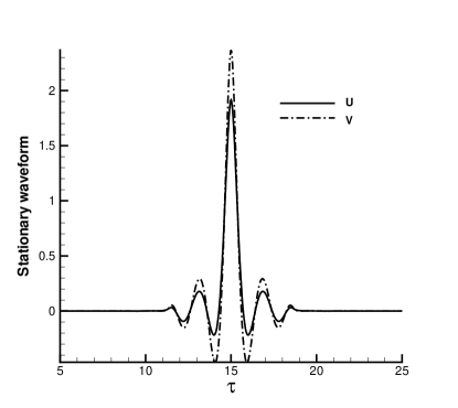
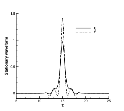
Figure 1: Examples of stable bimodal solitons with the single central peak. The total energy of the soliton, defined as per Eq. (7), is $E=5$ in (a) and $E=2$ in (b), respectively. The other parameters are $D_{2}=0.37,$ $c=0$, and the ratio of the wavenumbers of the two components is $R\equiv K_{v}/K_{u}=1.13$ in both cases.

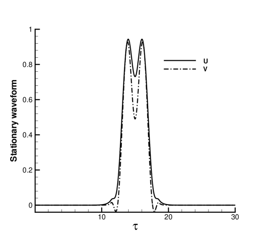
Figure 2: An example of a stable double-hump soliton found at the same values of parameters as in Fig. 1(a), including the total energy and the wavenumber ratio.

Further, Fig. 3 shows that, in either case (single- or double-peak structure), the solitons develop slowly decaying oscillatory tails as the relative GVD coefficient in Eq. (2), $D_{2}$, takes smaller values. In fact, the problem posed by strong tails in bimodal systems with (slightly) normal GVD in one component is well known in the studies of optical models with the $\chi^{(2)}$ nonlinearity, as in the cases of practical interest $\chi^{(2)}$ crystals feature normal GVD at the second harmonic chi2 . While, strictly speaking, the tail in the normal-GVD component cannot vanish at $\tau\rightarrow\pm\infty$, it has been concluded that one can identify a well-defined region in the respective parameter space, including a finite interval of negative values of $D_{2}$ (in the present notation), where the amplitude of the normal-GVD field assumes so small values at $\tau\rightarrow\infty$ that the nonvanishing portion of the tail is invisible and may be regarded as nonexistent, for all practical purposes. A transition from this case to the situation with a conspicuous long-range tail is sharp, and may be easily identified Isaac ; Kale ; we1 . In the present model, the tail is also, strictly speaking, nonvanishing in the case shown in Fig. 3(b), which pertains to $D_{2}=-0.3$. However, the figure demonstrates that, in practical terms, the tail is absent at large values of $|\tau|$.

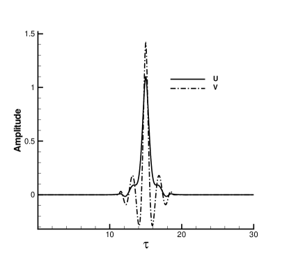
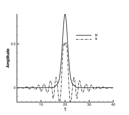
Figure 3: Examples of stable stationary solitons demonstrating the growth of the “tails” with the decrease of the GVD coefficient in the second component, $D_{2}$, at $c=0$, $E=2,$ $R=2.$ In (a) and (b), $D_{2}=0.1$ and $D_{2}=-0.3$, respectively.

Note that Fig. 3(b), which features, in addition to the well-developed tails, a slightly split peak in the $v$ component, also illustrates the transition between the single-hump and dual-hump types of the solitonic shape. Particular values of the scaled parameters for which Figs. 1-3 have been plotted (as indicated in captions to the figures) were taken pursuant to typical values of physical parameters in the lossless Drude model, which was used in Ref. Zhou to derive the coupled system of Eqs. (1) and (2) for the bimodal propagation of electromagnetic waves in the region of the negative refractive index.

Unlike the situation for simple fundamental solitons which was considered for $D_{2}=1$ variational , the variational approximation (VA) for solitons is not helpful in the present case, as one would have to use a complex ansatz approximating the oscillatory tails, as well the possibility of having the split peak at the center of the soliton. The use of the VA for the description of “tailed” gap solitons in the model with the self-defocusing nonlinearity and periodic potential (optical lattice) Arik , as well as for the transition from unsplit to split solitons profiles in two-component models Sadhan , has demonstrated that this may be possible in a limited range of parameters, but the necessary calculations are quite cumbersome. Actually, direct numerical solutions may be easier to obtain in this case than their VA counterparts.

The knowledge of the exact shape of the solitons may be essential for experiments, as the available size of MM samples, as well as the size of PCs, may be quite small, hence the transmission distance in the sample may not be long enough to allow self-shaping of the input signal into the soliton. Therefore, to observe and use the soliton propagation, it may be necessary to prepare an input pulse (in the case of the MM) or spatial beam (to be coupled into a PC) whose shape is as close as possible to that of the stable soliton, thus minimizing detrimental shape oscillations in the course of the transmission.

II.3 Stability regions

The stability of all the stationary solitons was tested by means of direct simulations of the propagation within the framework of Eqs. (1) and (2), adding small perturbations to the initial profile. As a result, it has been concluded that all the solitons which could be found in the stationary form, as reported above, are stable, including those with extended tails, which were found at small positive and negative values of $D_{2}$. Moreover, it has been concluded that the propagation distance necessary for the self-healing of weakly perturbed solitons and their relaxation back to the unperturbed shape was always essentially smaller than $z=10$ (in the present notation). Examples of the stable evolution of solitons with complex shapes, which feature strong tails or the split-peak structure, are displayed below in Fig. 8, see also other relevant examples in Figs. 5 and 10(a).

Thus, the stability region for the bimodal solitons is supposed to be identical to their existence area. For fixed material constants, $D_{2}$ and $c$ (actually, in this section we consider the case of $c=0$), soliton families depend on two intrinsic parameters, that may be identified as their wavenumbers $K_{u}$ and $K_{v}$, or, more conveniently, as the total energy, $E$, and the wavenumber ratio, $R=K_{v}/K_{u}$. An adequate rendition of the existence areas for the solitons of both types that were defined above, i.e., single- and double-hump ones, is provided by plotting the areas in the plane of $\left(E,D_{2}\right)$ at fixed values of $R$. In Fig. 4, we display overlapping existence regions of both soliton species for two characteristic values of the wavenumber ratio, $R=2$ and $1.2$. The large region of the bistability is evident in this figure.

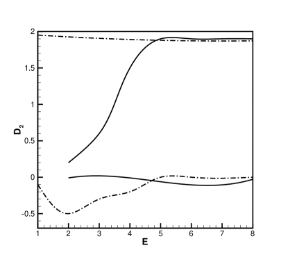
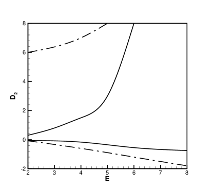
Figure 4: Borders of the regions of the existence (and, presumably, stability) for the single-peak and double-peak solitons, in the model with $c=0$ (zero group-velocity mismatch) are shown by dashed-dotted and continuous lines, respectively. Panels (a) and (b) correspond to fixed values of the wavenumber ratio: $R\equiv K_{v}/K_{u}=2$ in (a), and $R=1.2$ in (b). The overlap of the stability areas for both species of the solitons demonstrates the bistability of the system. In parts of the existence regions located at $D_{2}<0$ the $v$-component of the solutions, strictly speaking, cannot take a localized form. In fact, the bottom existence border separates the solutions which are “practically localized” and those with conspicuous tails, that do not vanish in the entire integration domain. For that reason, extension of the domain may lead to slight expansion of the existence region. There is no right border for the existence of the solitons, as they persist to indefinitely large values of the energy.

As one approaches the upper existence border for the solitons of either type, increasing $D_{2}$ at a fixed value of total energy $E$, the energy ratio, $E_{v}/E_{u}$ (see Eq. (5)), decreases, vanishing at the upper border. Above this border, only single-component solitons exist, with $v=0$ (of course, these are regular single-peak NLS solitons). The opposite trend is observed with the decrease of $D_{2}$ at fixed $E$: as one approaches the lower existence border, the $u$-component of the soliton tends to vanish, along with its energy share, while the $v$-component develops strong tails, especially in parts of the existence region located at $D_{2}<0$. It is easy to explain these trends, looking at the Hamiltonian of the present model (with $c=0$),

$$H=\int_{-\infty}^{+\infty}\left[(1/2)\left(\left|u_{\tau}\right|^{2}+D_{2}\left|v_{\tau}\right|^{2}+|u|^{4}+|v|^{4}\right)+2|uv|^{2}\right]d\tau.$$ (8)

Indeed, the minimization of the gradient part of the Hamiltonian at fixed $E$ is obviously favored by the attenuation of the $v$-component for large $D_{2}$, and by the decay of the $u$-component for small $D_{2}$. Another feature observed in Fig. 4 is the shrinkage of the existence regions for the double-hump solitons as the wavenumber ratio approaches $R=1$ (as suggested by the comparison of the panels appertaining to $R=2$ and $R=1.2$). At $R=1$ (equal wavenumbers in the two component), the system gives rise to single-hump solitons only.

A mathematically rigorous approach to the stability analysis for the solitons is based on the computation of the corresponding eigenvalues, using equations for perturbation modes linearized around the stationary soliton solutions. In particular, in Ref. aboutMoti2 is was concluded that all multi-hump solitons may be unstable, in this sense, in the case of $D_{2}=1$. On the other hand, our direct simulations of the evolution of double-hump solitons did not reveal any tangible instability at $D_{2}=1$ (note that line $D_{2}=1$ goes across the solitons’ existence regions in Fig. 4): weakly perturbed solitons remain apparently stable in this case, while a strong perturbation excites intrinsic vibrations in the soliton, but does not destroy it, see an example in Fig. 5. A possible explanation to these findings (thanks to which the solitons are classified here as stable also at $D_{2}=1$) is that the respective instability eigenvalues may be very small.

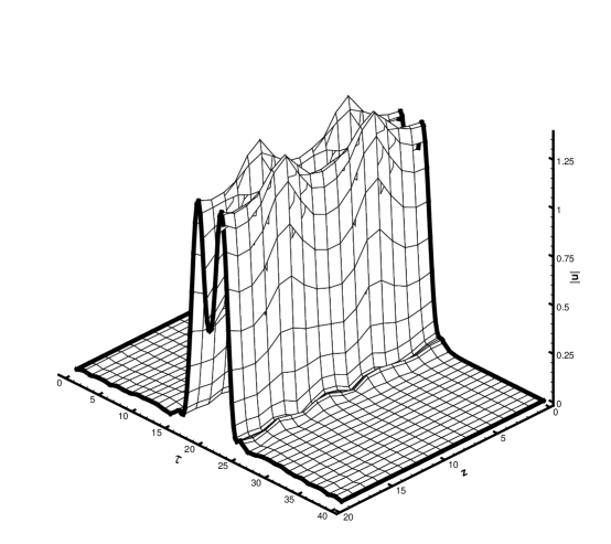
Figure 5: The perturbed evolution of the soliton for $D_{2}=1$, when its energy, $E=5$, was suddenly increased by $5\%$. The wavenumber ratio  of the unperturbed soliton is $R=2$.

II.4 The split-step method and “tailed” solitons

As said above, the application of the pseudospectral simulation algorithm readily corroborates the stability of all solitons that can be found in the stationary form, including those which feature conspicuous “tails” (see, e.g., Fig. 3). On the other hand, it is relevant to mention that the popular split-step-fast-Fourier-transform (SSFFT) method may produce numerical problems in the case of strong “tails”. An example of this is shown in Figs. 6 and 7, which demonstrate the difference in the numerical stability of the SSFFT algorithm in the absence of well-pronounced tails, and in cases when they are present.

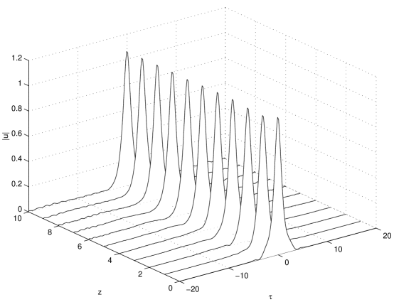
Figure 6: Results of the application of the split-step fast-Fourier-transform (SSFFT) method to the simulation of the evolution of a single-peak soliton without well-pronounced “tails”, for $D_{2}=0.3$ and $E=2$, $R\equiv E_{v}/E_{u}=2$. In this case, the SSFFT algorithm is relatively stable.

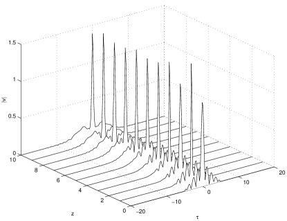
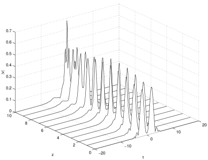
Figure 7: Unstable operation of the SSFFT algorithm simulating the evolution of a single-peak soliton with conspicuous tails (a), and a double-peak soliton (b). In both cases, the relative-GVD coefficient in Eq. (2) is $D_{2}=0.1$, and the initial solitons have $E=2$ and $R\equiv K_{u}/K_{u}=2$.

We stress that the evolution of the solitons was simulated by means of the SSFFT without adding any initial perturbations, i.e., Figs. 7(a) and (b) display results generated by an intrinsic instability of the algorithm when it is applied to the tailed and double-hump solitons. The SSFFT was realized, in these examples, covering the integration domain by 2048 points.

In fact, the solitons which were used as initial conditions in Figs. 6 and 7 are fully stable. To demonstrate this, in Fig. 8 we display simulations of the same pair of solitons as in Fig. 7, but performed by means of the pseudospectral algorithm which was outlined above.

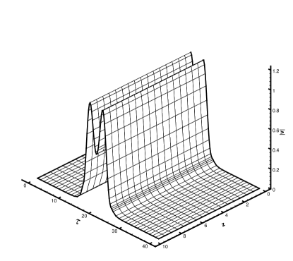
Figure 8: Simulations of the same initial solitons as in Fig. 7, but carried out by means of the stable pseudospectral method.

II.5 Effects of the loss and its compensation

As said above, dissipative effects may be negligible under experimentally relevant conditions in some types of artificial optical media, such as PCs and PC fibers, but they constitute an essential ingredient in the description of the light transmission through MMs loss ; necessary-loss . In the simplest approximation, the loss is taken into account by means of a positive dissipative coefficient, $\alpha$, added to Eqs. (1) and (2):

$$iu_{z}+(1/2)u_{\tau\tau}+\left(|u|^{2}+2|v|^{2}\right)u = -i\alpha u,$$ (9)

$$iv_{z}+icv_{\tau}+(1/2)D_{2}u_{\tau\tau}+\left(|v|^{2}+2|u|^{2}\right)v = -i\alpha v.$$ (10)

Obviously, the action of the loss leads to the decrease of the soliton’s energy. As seen in Fig. 4, the gradual decrease of the total energy should drive the solitons in the direction of the transition from the double-hump shape to the single-hump one, i.e., the loss is expected to make the solitons’ shape “more primitive”. This expectation is corroborated by a typical example of the evolution of the soliton under the action of the loss displayed in Fig. 9(a): under the action of the loss, the soliton gradually decays, transiting from the “tailed” shape to a tailless one.

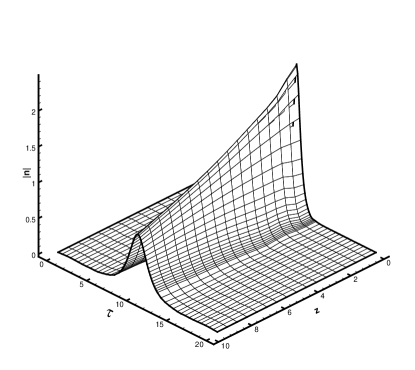
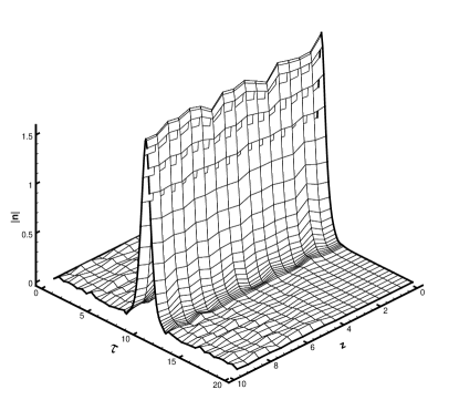
Figure 9: (a) Evolution of a typical soliton, with an originally “tailed” shape, initial total energy $E_{0}=5$, and $R_{0}\equiv K_{v}/K_{u}=1.13$, under the action of the loss with $\alpha=0.05$ and $D_{2}=0.37$ in Eqs. (9) and (10). (b) The same, but with the compensation of the loss by means of the instantaneous linear amplification, applied with period $\Delta z=1$.

As mentioned above, a number of works considered possibilities to periodically compensate the loss in MMs by an optical gain Shalaev ; matched-impedance ; gain . In Fig. 9 we display an example of that, assuming that, after passing each interval $\Delta z=1$, fields $u(\tau)$ and $v(\tau)$ are multiplied by a common factor $G=\exp\left(\alpha\Delta z\right)$, whose value is selected so as to compensate the loss in Eqs. (9) and (10). It is seen from the figure that the periodic compensation may readily maintain the soliton’s tailed shape.

III Stabilization of solitons by means of the group-velocity-mismatch management

In this work, we do not aim to find numerically exact complex (chirped) stationary solutions that may exist in the presence of the GVM, $c\neq 0$ (such solutions are known in the $\chi^{(2)}$ model with the GVM between the fundamental and second harmonics, which is related to the existence of “walking” $\chi^{(2)}$ solitons walking , and also in the system of coupled cubic NLS equations describing the co-propagation of orthogonal linearly-polarized modes in optical fibers, that includes, in addition to the XPM interaction, the nonlinear coupling via the four-wave mixing Torner ). Actually, it would be quite difficult to prepare such a pulse with a specific distribution of the internal chirp for the use in the experiment. On the other hand, an experimentally relevant problem is to simulate the evolution of the previously found stationary solitons in the framework of Eqs. (1) and (2) that include the GVM term. To this end, in Fig. 10(a) we display an example of the evolution of the soliton in the presence of relatively weak GVM (the particular value, $c=-0.144$, used in this figure, corresponds to physically relevant parameters as per the above-mentioned lossless Drude model Zhou ). It is seen that, while generating a permanent perturbation of the soliton, the moderate GVM term does not destroy it. On the other hand, Fig. 10(b) demonstrates that stronger GVM, with $c=1$, gives rise to a very strong perturbation, under which the soliton cannot maintain its integrity, even in an approximate form.

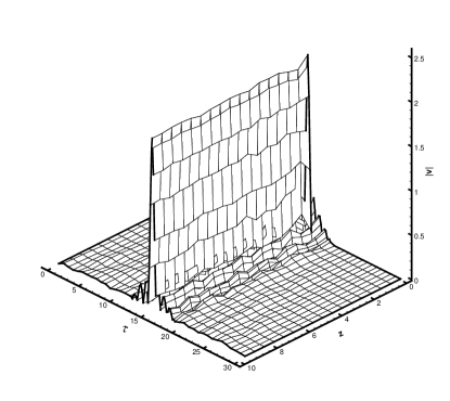
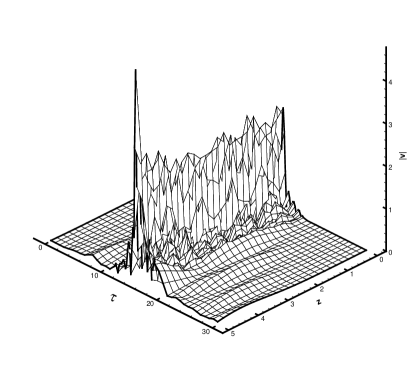
Figure 10: Evolution of solitons in the presence of the group-velocity-mismatch term, with $c=-0.144$ (a) or $c=-1$ (b). Other parameters are $D_{2}=0.37$ and $E=5,~{}R\equiv K_{v}/K_{u}=1.13$.

Because MMs and PCs are artificially built media, it may be quite natural to consider possibilities to engineer superstructures in them that can implement the GVM management, i.e., periodic alternation of layers with large GVM coefficients of opposite signs. In this way, it turns out easy to stabilize solitons against the locally strong GVM, provided that the management period, $L$, is relatively small in comparison with the effective wavelength, $\lambda_{v}\equiv 2\pi/K_{v}$. A typical example of the stabilization is displayed in Fig. 11. The scheme used in this figure is based on the following management map, with the zero average value of the GVM coefficient:

$$c(z)=\left\{\begin{array}[]{c}-1,~{}0<z<L/4,\\ +1,~{}L/4<z<3L/4,\\ -1,~{}3L/4<z<L,\end{array}\right.$$ (11)

which repeats with period $L.$ In the case shown in Fig. 11, $L=0.2$, which amounts to $\lambda_{v}/4$.  

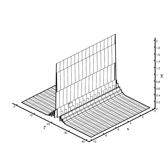
Figure 11: The stabilization of the same soliton as in Fig. 10 provided by the GVM-management scheme based on map (11) with $L=0.2=0.25\cdot\left(2\pi/K_{v}\right)$.

Finally, it is relevant to mention that, except for the case of $D_{2}=1$ in Eq. (2), the system as a whole does not support the Galilean invariance, therefore moving solitons may be essentially different from the quiescent ones, that were considered above. However, the study of moving localized solutions within the framework of Eqs. (1) and (2) is actually tantamount to considering solitons under the action of the GVM effect.

IV Conclusion

The objective of this work was to study solitons in a model based on the system of two XPM-coupled NLS equations, which describes the co-propagation of two waves in MMs (metamaterials), if the loss may be neglected, and in PCs (photonic crystals). The same system is relevant for ordinary optical fibers, close to the zero-dispersion point. The main peculiarity of the system is the small positive or negative value of the GVD coefficient in one equation, while the dispersion is fixed to be anomalous in the other. Unlike previously studied systems of nonlinearly coupled NLS equations with equal GVD coefficients, which gives rise only to simple stable single-peak solitons with an arbitrary ratio of the energy between the components, the present model generates soliton families which feature complex shapes, including those with weakly localized oscillatory tails and a double-peak maximum. Existence regions for the single- and double-peak solitons have been identified in the parameter planes, demonstrating a broad range of the bistability in the system. Above the upper existence border, the two-component solitons degenerate into obvious single-component fundamental NLS solitons. Systematic direct simulations demonstrate that solitons of both types are stable throughout their existence regions. Under the action of the loss, the decaying solitons tend to evolve towards more “primitive” shapes, losing their tails. On the other hand, the periodic compensation of the loss helps to maintain the original shape. The numerical calculations were performed by means of a properly adjusted pseudospectral method (while the usual split-step algorithm may be problematic when applied to simulating the evolution of solitons with conspicuous tails). The extended model, including the GVM (group-velocity mismatch) was studied too. It has been demonstrated that, while a sufficiently strong GVM term tends to destroy the bimodal solitons, they can be readily stabilized by way of the GVM-management scheme.

This work suggests extensions in several directions. First, a study of collisions between moving solitons may be a natural addition to the above analysis. Dispersion management my-book may also be considered in the framework of the present model. On the other hand, the model can be made two- and three-dimensional by adding transverse coordinates. In that case, a challenging issue would be a possibility to stabilize the respective spatiotemporal solitons (“light bullets”) against the collapse by means of a grating created in the transverse direction(s), as well as by means of the respectively modified dispersion-management scheme, cf. Ref. Warsaw .

References

- (1) T. F. Krauss, R. M. De La Rue, S. Brand, Nature 383 (1996) 699; J. E. G. J. Wijnhoven, W. L. Vos, Science 281 (1998) 802; C. P. Collier, T. Vossmeyer, J. R. Heath, Ann. Rev. Phys. Chem. 49 (1998) 371; R. J. Warburton, C. Schaflein, D. Haft D, F. Bickel, A. Lorke, K. Karrai, J. M. Garcia, W. Schoenfeld, P. M. Petroff, Nature 405 (2000) 926; S. Link, M. A. Ei-Sayed, Ann. Rev. Phys. Chem. 54 (2003) 331; A. N. Grigorenko, A. K. Geim, H. F. Gleeson, Y. Zhang, A. A. Firsov, I. Y. Khrushchev, J. Petrovic, Nature 438 (2005) 335.
- (2) J. B. Pendry, D. R. Smith, Phys. Today 57 (2004) 37.
- (3) J. B. Pendry, Phys. Rev. Lett. 85 (2000) 3966; N. Fang, H. Lee, C. Sun, X. Zhang, Science 308 (2005) 534;Z. Jacob, L. V. Alekseyev, E. Narimanov , Opt. Exp. 14 (2006) 8247.
- (4) V. M. Shalaev, Nature Photonics 1 (2007) 41.
- (5) V. G. Veselago, Sov. Phys. Usp. 10 (1968) 509.
- (6) J. B. Pendry, A. J. Holden, D. J. Robbins, W. J. Stewart, IEEE Trans. Microwave Theory Tech. 47 (1999) 2075; S. O. O’Brien, D. McPeake, S. A. Ramakrishna, J. B. Pendry, Phys. Rev. B 69 (2004) 241101(R); A. A. Zharov, I. V. Shadrivov, Y. S. Kivshar, Phys. Rev. Lett. 91 (2003) 03401; I. R. Gabitov, R. A. Indik, N. M. Litchinitser, A. I. Maimistov, V. M. Shalaev, J. E. Soneson, J. Opt. Soc. Am. 23 (2006) 535;N. M. Litchinitser, I. R. Gabitov, A. I. Maimistov, V. M. Shalaev, Opt. Lett. 32 (2007) 151;N. M. Litchinitser , I. R. Gabitov, A. I. Maimistov, Phys. Rev. Lett. 99 (2007) 113902.
- (7) A. I. Maimistov and I. R. Gabitov, Eur. Phys. J. Special Topics 147 (2007) 265.
- (8) M. Scalora, M. S. Syrchin, N. Akozbek, E. Y. Poliakov, G. D’Aguanno, N. Mattiucci, M. J. Bloemer, A. M. Zheltikov, Phys. Rev. Lett. 95 (2005) 013902; P. P. Banerjee, G. Nehmetallah, J. Opt. Soc. Am. B 23 (2006) 2348; P. P. Banerjee, G. Nehmetallah, J. Opt. Soc. Am. B 24 (2007) A69.
- (9) W. Zhou, W. Su, X. Cheng, Y. Xiang, X. Dai, S. Wen, Opt. Commun. 282 (2009) 1440.
- (10) M. Scalora, G. D’Aguanno, M. Bloemer, M. Centini, D. de Ceglia, N. Mattiucci, Y. S. Kivshar, Opt. Exp. 14 (2006).
- (11) V. Roppo, M. Centini, C. Sibilia, M. Bertolotti, D. de Ceglia, M. Scalora, N. Akozbek, M. J. Bloemer, J. W. Haus, O. G. Kosareva, V. P. Kandidov, Phys. Rev. A 76 (2007) 033829.
- (12) A. D. Boardman, P. Egan, L. Velasco, N. King, J. Opt. A: Pure Appl. Opt. 7 (2005) S57.I. V. Shadrivov, Y. S. Kivshar, J. Opt. A: Pure Appl. Opt. 7 (2005) S68;N. A. Zharova, I. V. Shadrivov, A. A. Zharov, Opt. Exp. 13 (2005) 129;M. Marklund, P. K. Shukla, L. Stenflo, G. Brodin, Phys. Lett. A 341 (2005) 231;S. C. Wen, Y. J. Xiang, W. H. Su, Y. H. Hu, X. Q. Fu, D. Y. Fan, Opt. Exp. 14 (2006) 1568;Y. M. Liu, G. Bartal, D. A. Genov, X. Zhang, Phys. Rev. Lett. 99 (2007) 153901; I. Kourakis, N. Lazarides, G. P. Tsironis, Phys. Rev. E 75 (2007) 067601.
- (13) G. P. Agrawal, Phys. Rev. Lett. 59 (1987) 880.G. P. Agrawal, P. L. Baldeck, R. R. Alfano, Phys. Rev. A 39 (1989) 3406.
- (14) B. A. Malomed, Phys. Rev. E 50 (1994) 1565.
- (15) A. Ferrando, E. Silvestre, P. Andrés, J. J. Miret, M. V. Andrés, Opt. Exp. 9 (2001) 687;T. M. Monro, D. J. Richardson, Comptes Rendus Phys. 4(2003) 175.
- (16) J. D. Joannopoulos, S. G. Johnson, J. N. Winn, R. D. Meade, Photonic crystals: molding the flow of light (Princeton University Press: Princeton and Oxford, 2008).
- (17) R. W. Ziolkowski, E. Heyman, Phys. Rev. E 64 (2001) 056625; A. Alu, N. Engheta, Phys. Rev. E 72 (2005) 016623; G. Dolling, C. Enkrich, M. Wegener, C. M. Soukoulis, S. Linden, Opt. Lett. 31 (2006) 1800;N. M. Litchinitser, V. M. Shalaev, Nature Photonics 3 (2009) 75.
- (18) M. I. Stockman, Phys. Rev. Lett. 98 (2007) 177404.
- (19) V. M. Shalaev, W. Cai, U. K. Chettiar, H. Yuan, A. K. Sarychev, V. P. Drachev, A. V. Kildishev, Opt. Lett. 30 (2005) 3356.
- (20) A. K. Popov, V. M. Shalaev, Opt. Lett. 31 (2006) 2169; A. D. Boardman, Yu. G. Rapoport, N. King, V. N. Malnev, J. Opt. Soc. Am. B 24 (2007) A53;J. A. Gordon, R. W. Ziolkowski, Opt. Exp. 15 (2007) 2622.A. K. Sarychev, G. Tartakovsky, Phys. Rev. B 75 (2007) 085436; M. A. Noginov, V. A. Podolskiy, G. Zhu, M. Mayy, M. Bahoura, J. A. Adegoke, B. A. Ritzo, K. Reynolds, Opt. Exp. 16 (2008) 1385.
- (21) P. Tassin, L. Gelens, J. Danckaert, I. Veretennicoff , G. Van der Sande, P. Kockaert, M. Tlidi, Chaos 17 (2007) 037116.
- (22) A. Shipulin, G. Onishchukov, B. A. Malomed, J. Opt. Soc. Am. B 14 (1997) 3393;B. A. Malomed A. Shipulin, Opt. Commun. 162 (1999) 140.
- (23) D. N. Christodoulides and R. I. Joseph, Opt. Lett. 13 (1988) 53; M. Haelterman, A. P. Sheppard, A. W. Snyder, Opt. Lett. 18 (1993) 1406.
- (24) T. Ueda, W. L. Kath, Phys. Rev. A 42 (1990) 563;D. J. Kaup, B. A. Malomed, R. S. Tasgal, Phys. Rev. E 48 (1993) 3049;B. A. Malomed, R. S. Tasgal, Phys. Rev. E 58 (1998) 2564.
- (25) J. Yang, Physica D 108 (1997) 92.
- (26) D. E. Pelinovsky, J. Yang, Stud. Appl. Math. 115 (2005) 109.
- (27) M. Mitchell, M. Segev, T. H. Coskun, D. N. Christodoulides, Phys. Rev. Lett. 79 (1997) 4990.
- (28) M. Mitchell, M. Segev, D. N. Christodoulides, Phys. Rev. Lett. 80 (1998) 4657.
- (29) E. A. Ostrovskaya, Y. S. Kivshar, D. V. Skryabin, W. J. Firth, Phys. Rev. Lett. 83 (1999) 296.
- (30) T. Carmon, C. Anastassiou, S. Lan, D. Kip, Z. H. Musslimani, M. Segev, D. Christodoulides, Opt. Lett. 25 (2000) 1113;Z. H. Musslimani, M. Segev, D. N. Christodoulides, M. Soljacic, Phys. Rev. Lett. 84 (2000) 1164.
- (31) C. R. Menyuk, R. Schiek, L. Torner, J. Opt. Soc. Am. B 11 (1994) 2434;P. Di Trapani, D. Caironi, G. Valiulis, A. Dubietis, R. Danielius, A. Piskarskas, Phys. Rev. Lett. 81 (1998) 570;X. Liu, L. J. Qian, F. W. Wise, Phys. Rev. Lett. 82 (1999) 463.
- (32) K. Beckwitt, Y. F. Chen, F. W. Wise, B. A. Malomed, Phys. Rev. E 68 (2003) 057601.
- (33) P. Y. P. Chen, B. A. Malomed, Opt. Commun. 281 (2008) 5257;P. Y. P. Chen, B.A. Malomed, Stabilization of spatiotemporal solitons in second-harmonic-generating media, Opt. Commun., in press.
- (34) L. Torner, IEEE Phot. Tech. Lett. 11 (1999) 1268;L. Torner, S. Carrasco, J. P. Torres, L. C. Crasovan, D. Mihalache, Opt. Commun. 199 (2001) 277;S. Carrasco, D. V. Petrov, J. P. Torres, L. Torner, H. Kim, G. Stegeman, J. J. Zondy, Opt. Lett. 29 (2004) 382.
- (35) D. Gottlieb, S. A. Orszag, Numerical Analysis of Spectral Method: Theory and Applications (SIAM: Philadelphia, 1977); G. Cohen, S. Fanqueux, SIAM J. Sci. Comput. 26 (2005) 864.
- (36) M. Dehghan, A. Taleei, Numerical Methods for Partial Differential Equations, in press (2009; DOI 10.1002/num.20468).
- (37) O. V. Sinkin, R. Holzlohner, J. Zweck, C. R. Menyuk, J. Lightwave Tech. 21 (2003) 61.
- (38) I. N. Towers, B. A. Malomed, F. W. Wise, Phys. Rev. Lett. 90 (2003) 123902.
- (39) A. Gubeskys, B. A. Malomed, I. M. Merhasin, Stud. Appl. Math. 115 (2005) 255; H. Sakaguchi and B. A. Malomed, Phys. Rev. A 79 (2009) 043606.
- (40) S. K. Adhikari, B. A. Malomed, Phys. Rev. A 77 (2008) 023607.
- (41) L. Torner, D. Mazilu, D. Mihalache, Phys. Rev. Lett. 77 (1996) 2455;U. Peschel, F. Lederer, and B. A. Malomed, Phys. Rev. E 55 (1997) 6155.
- (42) D. Mihalache, D. Mazilu, L. Torner, Phys. Rev. Lett. 81 (1998) 4353.
- (43) B. A. Malomed, Soliton management in Periodic Systems (Springer: New York, 2006).
- (44) M. Matuszewski, M. Trippenbach, B. A. Malomed, E. Infeld, M. Skorupski, Phys. Rev. E 70 (2004) 016603.