An Integrated Analysis of Radial Velocities in Planet Searches

Abstract

We discuss a Bayesian approach to the analysis of radial velocities in planet searches. We use a combination of exact and approximate analytic and numerical techniques to efficiently evaluate $\chi^{2}$ for multiple values of orbital parameters, and to carry out the marginalization integrals for a single planet including the possibility of a long term trend. The result is a robust algorithm that is rapid enough for use in real time analysis that outputs constraints on orbital parameters and false alarm probabilities for the planet and long term trend. The constraints on parameters and odds ratio that we derive compare well with previous calculations based on Markov Chain Monte Carlo methods, and we compare our results with other techniques for estimating false alarm probabilities and errors in derived orbital parameters. False alarm probabilities from the Bayesian analysis are systematically higher than frequentist false alarm probabilities, due to the different accounting of the number of trials. We show that upper limits on the velocity amplitude derived for circular orbits are a good estimate of the upper limit on the amplitude of eccentric orbits for $e\la 0.5$.

1 Introduction

The analysis of a set of radial velocities in planet searches typically involves a number of different steps. First, the best fitting Keplerian orbital parameters are found by minimizing $\chi^{2}$, for example with a Levenberg-Marquardt algorithm (Press et al., 1992). Because of the complex multimodal shape of the $\chi^{2}$ distribution in parameter space, a Lomb-Scargle periodogram (Lomb, 1978; Scargle, 1982) is often used beforehand to fit circular orbits at a range of orbital periods, providing starting points for the Keplerian fit. Then the reality of the signal is assessed by calculating the false alarm probability (FAP) that the observed signal could arise due to noise fluctuations, typically using Monte Carlo simulations (Marcy et al., 2005; Cumming, 2004). This has become particularly important as radial velocity surveys reveal planets with lower velocity amplitudes, comparable to the measurement uncertainties and other sources of noise. A related question is comparing different models for the data, for example deciding whether a two (or more) planet model is preferred over a single planet model, or whether to include a long term trend due to a long period companion (see for example, Robinson et al. 2007).

Uncertainties in the fitted orbital parameters are then calculated. A common technique is to scramble the residuals to the best fit Keplerian orbit, add them back to the predicted velocity curve, and refit the orbit. After repeating this many times, the distribution of fitted parameters gives an estimate of the uncertainty (Marcy et al., 2005). Another approach is to use Bayesian methods implemented with Markov Chain Monte Carlo (MCMC) simulations (Ford, 2005). In the case of a non-detection, the upper limit on the planet mass as a function of orbital period is an important input for population studies (Walker et al., 1995; Cumming et al., 1999; Endl et al., 2002; Wittenmyer et al., 2006).

Often, all of these steps must be carried out for a given radial velocity data set. Many of them are based on Monte Carlo simulations involving fitting Keplerian orbits to synthetic data sets. These trials can become cumbersome for the large numbers of orbital frequencies that must be considered. For this reason, recent calculations have produced upper limits for circular orbits only (Cumming et al., 2008), relying on the fact that detectability of planets falls off with eccentricity only for $e\ga 0.6$ (Endl et al., 2002; Cumming, 2004), or on a sparse grid of orbital period values (O’ Toole et al. 2008).

We focus in this paper on a Bayesian approach to the analysis of radial velocity data. The advantage is that, in principle, a Bayesian analysis answers all of the above questions with a single calculation, providing constraints on model parameters and odds ratios which can be used to decide which model best describes the data (Ford, 2005; Gregory, 2005b; Cumming, 2004). This would simplify analysis of radial velocity data sets. The difficulty in practice is that the marginalization over parameters requires the evaluation of multidimensional integrals over parameter space.

Bayesian methods have been applied to planet searches, using sophisticated Markov Chain Monte Carlo (MCMC) techniques to evaluate the integrals. Ford (2005) applied this technique to determining the constraints on orbital parameters, while Gregory in a series of papers (Gregory, 2005b, 2007a, 2007b) also considers model comparison. Ford (2006) investigated different proposal distribution functions to help speed convergence of MCMC chains. Whereas the chains used by Ford (2005) were $10^{6}$–$10^{10}$ steps in length, Ford (2006) found that it was possible to achieve convergence after only $10^{4}$–$10^{6}$ steps by optimizing the directions in parameter space in which steps are taken. Recently, Balan & Lahav (2009) have developed an MCMC code Exofit based on the methodology of Ford & Gregory (2007) which is publicly available.

Despite this tremendous progress, the application of MCMC to radial velocity data is not yet routine, although it is commonly used to assess uncertainties in orbital parameters. As well as optimizing the steps in parameter space, one important difficulty in using the MCMC approach is assessing whether the chains have converged. Another is that when the signal to noise ratio is low and the distribution of $\chi^{2}$ in parameter space is multimodal, the MCMC chain may miss minima in $\chi^{2}$. Gregory (2005b) introduced a parallel tempering scheme in which several MCMC chains are run simultaneously, each with a different temperature, hotter chains making larger jumps in parameter space, colder chains exploring local minima. As the calculation progresses, the chains exchange information in a way that preserves their statistical character. This scheme has been successfully applied to multiple planet systems (Gregory, 2007a, b).

In this paper, we take a different approach. We consider models with one planet only, or one planet plus a long term linear trend, and use a combination of grid-based numerical evaluation and exact and approximate analytic methods to evaluate the marginalization integrals. The idea is to look for ways in which the marginalization integrals can be evaluated more efficiently. As well as providing a useful tool for analysing radial velocity data for single planet systems, it provides a check on the output of MCMC simulations, and may have application to making MCMC codes for analysis of multiple planet systems more efficient.

We start in §2 with an overview of the Bayesian approach, including how to write down the posterior probabilities for orbital parameters, and how to use them to calculate false alarm probabilities. In §3, we discuss circular orbits, using analytic techniques to evaluate the marginalization integrals. In §4, we divide the parameters for eccentric orbits into fast (linear) and slow (non-linear) parameters, and use the analytic techniques for circular orbits to marginalize over the fast parameters. In §5, we compare our results to MCMC calculations, and traditional methods for evaluating false alarm probabilities and upper limits on companion mass.

2 Overview

Bayesian analysis of radial velocity data has been discussed previously by several authors (Ford, 2005, 2006, 2008; Ford & Gregory, 2007; Gregory, 2005a, b, 2007a, 2007b; Cumming, 2004). Here we give a brief reminder of the basic ideas and introduce our notation, and show how the systemic velocity and noise uncertainty can be analytically marginalized.

2.1 Parameter estimation

We start with a model for the radial velocities with set of parameters $\vec{a}$. For example, a single Keplerian orbit has six parameters $\vec{a}=(K,P,e,\omega_{p},t_{p},\gamma)$, where $K$ is the velocity amplitude, $P$ the orbital period, $e$ the eccentricity, $\omega_{p}$ and $t_{p}$ are the argument and time of pericenter, and $\gamma$ is the systemic velocity. The data consist of a set of $N$ measured velocities $v_{i}$, observation times $t_{i}$, and errors $\sigma_{i}$. Bayes’ theorem allows us to calculate the probability distribution of the parameters $\vec{a}$ given the data, also known as the posterior probability of $\vec{a}$,

$${\mathcal{P}}\left(\vec{a}|d\right)={{\mathcal{P}}(\vec{a}){\mathcal{P}}(d|\vec{a})\over{\mathcal{P}}(d)},$$ (1)

where ${\mathcal{P}}(d)$ is a normalization factor. The term ${\mathcal{P}}(\vec{a})$ is the prior probability distribution for the parameters $\vec{a}$, which allows us to specify any knowledge of the parameter distribution that we have before the data are taken. If the errors are Gaussian-distributed and uncorrelated, the likelihood of the data, or probability of the data given a particular choice of model parameters is

$${\mathcal{P}}\left(d|\vec{a}\right)={1\over\prod_{i}(2\pi)^{1/2}\sigma_{i}}\exp\left({-{\chi^{2}(\vec{a})\over 2}}\right)$$ (2)

where

$$\chi^{2}(\vec{a})=\sum_{i=1}^{N}w_{i}\left(v_{i}-V_{i}(\vec{a})\right)^{2}$$ (3)

is the usual $\chi^{2}$ statistic, written in terms of weights $w_{i}=1/\sigma_{i}^{2}$. We write the model velocity at time $t_{i}$ as $V_{i}$.

Often, we are interested in the probability distribution of a single parameter, or a subset of parameters. For example, a circular orbit has $\vec{a}=(K,P,\gamma,\phi)$, where $K$ is the velocity amplitude, $P$ the orbital period, $\gamma$ the systemic velocity, and $\phi$ the orbital phase. It is likely that we are not interested in the particular values of $\gamma$ or $\phi$, but want to constrain the orbital period and velocity amplitude. The joint probability distribution for $P$ and $K$ can be obtained by marginalizing over the other parameters,

$${\mathcal{P}}(P,K|d)=\int d\phi\int d\gamma\ {\mathcal{P}}(P,K,\phi,\gamma|d).$$ (4)

Marginalization amounts to performing a weighted average of the probability distribution over the unwanted parameters.

A number of other useful quantities can be obtained from ${\mathcal{P}}(P,K|d)$. Further integration over $K$ gives ${\mathcal{P}}(P|d)$, or integration over $P$ gives ${\mathcal{P}}(K|d)$. A confidence interval for $K$ can be calculated from ${\mathcal{P}}(K|d)$. For example, if a planet is not detected in a given data set, an upper limit can be placed on the amplitude of undetected orbits. The 99% upper limit $K_{99}$ is given by $\int_{0}^{K_{99}}dK{\mathcal{P}}(K|d)/\int_{0}^{\infty}dK{\mathcal{P}}(K|d)=0.99$.

For eccentric orbits, we will focus in this paper on obtaining ${\mathcal{P}}(P,e,K|d)$ by marginalizing over $\gamma$, $\omega_{p}$, and $t_{p}$.

2.2 The noise distribution

In equation (2), we assumed that the standard deviation of the noise for each observation $\sigma_{i}$ was given. In reality, other noise sources may be present in the data that hinder the identification of planetary signals, for example intrinsic stellar “jitter” (e.g. Wright 2005) due to rotation of spots across the surface of the star, or changes in line profiles over time related to magnetic activity. This extra noise can be incorporated as an additional parameter of the model. A common choice (Gregory 2005b; Ford 2006) is to add the extra noise term in quadrature with the measurement errors $\sigma_{i}$.

Here, we instead multiply each value of $\sigma_{i}$ by a noise scaling factor $k$ (Cumming, 2004; Gregory, 2005a), and analytically marginalize over $k$ (e.g. Sivia 1996)

$${\mathcal{P}}(d|\vec{a})\propto\int_{0}^{\infty}{dk\over k}{1\over k^{N}}\exp\left(-{\chi^{2}(\vec{a})\over 2k^{2}}\right)\propto\left(\chi^{2}(\vec{a})\right)^{-N/2}.$$ (5)

The constant prefactor, which depends only on the weights $w_{i}$ and the number of observations $N$, does not affect the shape of the posterior probability distributions, and cancels out when we calculate odds ratios. Therefore, we drop it and replace equation (2) with

$${\mathcal{P}}(d|\vec{a})=\left(\chi^{2}(\vec{a})\right)^{-N/2}.$$ (6)

This is a Student’s t-distribution rather than Gaussian distribution (Sivia, 1996).

We take an infinite range for $k$ in equation (5), whereas in reality we likely have some information about the uncertainty in the noise level. For example, we may be able to estimate the size of the expected stellar jitter based on stellar properties (Wright, 2005). Alternatively, we could keep $k$ as a parameter, and evaluate the constraints on $k$ from the data, ${\mathcal{P}}(k|d)$ (e.g. Ford 2006). We have tried marginalizing numerically over $k$ with finite limits, and find that the results for realistic ranges of $k$ are close to the analytic case with infinite limits. Therefore we marginalize analytically over $k$ and adopt equation (6) as the likelihood throughout this paper.

2.3 Priors

The choice of appropriate prior probabilities ${\mathcal{P}}(\vec{a})$ for the various parameters has been discussed in depth in the literature (e.g. Gregory 2005b; Ford & Gregory 2007). We mostly follow this previous work. For circular orbits, we use uniform priors for $\gamma$ and $\phi$, and priors for $K$,$P$ that are uniform in log (the Jeffreys prior). For eccentric orbits, we take uniform priors in $\gamma$, $t_{p}$, $\omega_{p}$, $e$, and log-uniform priors in $K$, and $P$, i.e. ${\mathcal{P}}(P)=1/(P\log(P_{2}/P_{1}))$ and ${\mathcal{P}}(K)=1/(K\log(K_{2}/K_{1}))$. If a long term trend is included in the model (a linear term $\beta t_{i}$; see Appendix A), we take a uniform prior in the slope $\beta$.

In fact, Gregory (2005b) and Ford & Gregory (2007) use a modified Jeffreys prior for the noise term and the velocity amplitude rather than the standard Jeffreys prior. A modified Jeffreys prior is uniform in log above some scale, and uniform below that scale. For radial velocity amplitude $K$ or extra noise term, the turnover scale is taken to be $\approx 1\ {\rm m/s}$. The values of $K$ we are interested in are typically larger than this, and so for simplicity we use a Jeffreys prior between our lower and upper limits in $K$. The ranges that we take are $K=1\ {\rm m/s}$ to $2\Delta v$, where $\Delta v$ is the observed range of velocities, and $P=1$ day to the time span of the observations.

2.4 Model comparison and the false alarm probability

Marginalizing over all the parameters of a model gives the total probability of that model. For example, given ${\mathcal{P}}(P,K|d)$ for circular orbits, we could calculate the total probability that a planet is present

$${\mathcal{P}}(1|d)=\int dP\int dK\ {\mathcal{P}}(P,K|d).$$ (7)

Similarly, by considering a model without a planet, we can calculate the probability that no planet is present given the data, ${\mathcal{P}}(0|d)$. We define the normalization ${\mathcal{P}}(d)$ in equation (1) so that the sum over the probabilities of all models is unity. For example, if we consider only two possible models, that there is or is not a planet present, we choose ${\mathcal{P}}(d)$ such that

$${\mathcal{P}}(1|d)+{\mathcal{P}}(0|d)=1.$$ (8)

We can think of the posterior probability that there is no planet present ${\mathcal{P}}(0|d)$ as the false alarm probability. It can be written without including the ${\mathcal{P}}(d)$ factors explicitly as

$$F={\mathcal{P}}(0|d)={1\over 1+\Lambda}$$ (9)

where $\Lambda$ is the odds ratio

$$\Lambda={{\mathcal{P}}(1|d)\over{\mathcal{P}}(0|d)}$$ (10)

(the normalization factors ${\mathcal{P}}(d)$ cancel out when the ratio is taken). For $\Lambda\gg 1$, $F\approx\Lambda^{-1}$. The odds ratio is

$$\Lambda={\int dK\int dP\ {\mathcal{P}}(P,K|d)\over{\mathcal{P}}(0|d)},$$ (11)

for circular orbits, or

$$\Lambda={\int dK\int dP\int de\ {\mathcal{P}}(P,K,e|d)\over{\mathcal{P}}(0|d)},$$ (12)

for eccentric orbits.

This approach can be generalized to more than two models. For example, later we will consider four possible models for a given star, the possible combinations of including or not including a Keplerian orbit with period less than the time span of the observations, and including or not including a long term trend. To calculate the false alarm probability associated with the short period planet, we define the odds ratio

$$\Lambda={{\mathcal{P}}(1|d)+{\mathcal{P}}(1,t|d)\over{\mathcal{P}}(0|d)+{\mathcal{P}}(0,t|d)}$$ (13)

where $1$ or $0$ indicate that the short period planet is or is not included in the model, and $t$ indicates that a long term trend is included.

2.5 Probability that there is no planet ${\mathcal{P}}(0|d)$

The posterior probability of no planet ${\mathcal{P}}(0|d)$, where the “no planet” model is a constant velocity $V_{i}=\gamma$, can be calculated analytically. Using the likelihood of equation (6)

$${\mathcal{P}}(0|d)={1\over{\mathcal{P}}(d)\Delta\gamma}\int_{\gamma_{1}}^{\gamma_{2}}\ d\gamma\ \left(\chi^{2}(\gamma)\right)^{-N/2}$$ (14)

where $\Delta\gamma=\gamma_{2}-\gamma_{1}$ is the range of values of $\gamma$ considered, and we assume a uniform prior for $\gamma$ in that range. Minimizing $\chi^{2}$ with respect to $\gamma$, we find the best-fitting value $\gamma_{0}=\sum w_{i}v_{i}/\sum w_{i}$. In terms of $\gamma_{0}$, we can write

$$\chi^{2}\left(\gamma\right)=\chi^{2}(\gamma_{0})+(\gamma-\gamma_{0})^{2}\sum w_{i}.$$ (15)

The fact that the distribution of $\chi^{2}(\gamma)$ is analytic is mentioned in Ford (2006). For clarity, we drop the subscript $i$ on the sum in equation (15) and in the remainder of the paper, a sum over the observations with $i$ running from $1$ to $N$ is implied.

The quadratic form of $\chi^{2}$ allows the integral over $\gamma$ to be carried out analytically when the limits $\gamma_{1}\rightarrow-\infty$ and $\gamma_{2}\rightarrow\infty$. In that limit, the normalization factor diverges, $\Delta\gamma\rightarrow\infty$. However the values of $\Delta\gamma$ cancel when we form an odds ratio, as does the normalization factor ${\mathcal{P}}(d)$. Therefore, we can drop the prefactor after integrating, giving the final result

$${\mathcal{P}}(0|d)=\left(\chi^{2}(\gamma_{0})\right)^{-(N-1)/2}.$$ (16)

An alternative “no planet” model is a linear trend in the radial velocities over time, $V_{i}=\gamma+\beta t_{i}$. A linear term is often included (and needed) in radial velocity fits to account for additional companions with long orbital periods. A similar formula for ${\mathcal{P}}(0|d)$ can be derived in that case. For clarity, we leave this to Appendix A, along with how to add a linear term to the circular and Keplerian orbit fits, and consider only the constant velocity no planet model in the main text.

3 Circular orbits

In the previous section, we saw that a calculation of ${\mathcal{P}}(\vec{a}|d)$ followed by successive marginalization provides constraints on all model parameters and a measure of the false alarm probability. The difficulty in practice is in performing the integrals over parameter space. We first consider circular orbits, which have a simple sinusoidal velocity curve, and introduce some analytic approximations that allow us to rapidly carry out these integrals. Apart from being a testing ground for these techniques which we will then apply to eccentric orbits, fitting circular orbits is actually quite useful since sinusoid fits are sufficient to detect orbits even with moderate eccentricities ($e\la 0.5$; Endl et al. 2002; Cumming 2004).

For a circular orbit, the model for the velocities is

$$V_{i}=\gamma+K\sin\left(\omega t_{i}+\phi\right)$$ (17)

which has four parameters: $\gamma$ is the systemic velocity, $K$ is the velocity semi-amplitude, $\phi$ the phase and $\omega=2\pi/P$ the orbital frequency, $P$ is the orbital period. Our aim in this section is to obtain ${\mathcal{P}}(P,K)$, marginalizing over $\gamma$ and $\phi$. We first marginalize analytically over $\gamma$ to obtain ${\mathcal{P}}(\phi,K,P|d)$, and then present two different methods for efficiently marginalizing over the parameters $K$ and $\phi$. The methods are summarized and applied to an example data set in §3.5.

3.1 Analytic marginalization of the systemic velocity

To integrate over $\gamma$, we note again that $\chi^{2}$ depends quadratically on $\gamma$ around the best-fit value, as given by equation (15), where this time $\gamma_{0}(\phi,K,P)$ is the best fit systemic velocity at each $\phi$, $P$ and $K$, that is $\gamma_{0}(\phi,K,P)$ is the value of $\gamma$ that minimizes $\chi^{2}$ at each $\phi$, $P$ and $K$, and $\chi^{2}(\gamma_{0})$ is the corresponding minimum value of $\chi^{2}$. The best-fit systemic velocity can be calculated from $\partial\chi^{2}/\partial\gamma=0$, giving

$$\gamma_{0}=\sum w_{i}\left[v_{i}-K\sin\left(\omega t_{i}+\phi\right)\right]/\sum w_{i}.$$ (18)

Adopting a uniform prior for $\gamma$ and integrating for $\Delta\gamma\rightarrow\infty$, we find

$${\mathcal{P}}\left(d|\phi,K,P\right)=\left(\chi^{2}\left[\gamma_{0},\phi,K,P\right]\right)^{-(N-1)/2},$$ (19)

where $\gamma_{0}(\phi,K,P)$ is given by equation (18), and we have set the prefactor equal to unity as in §2.5.

3.2 Evaluation of ${\mathcal{P}}(\phi,K,P|d)$ on a grid

Next, we describe a method for rapidly evaluating ${\mathcal{P}}(\phi,K,P|d)$ numerically for a grid of values of $\phi$, $K$, and $P$. We introduce the averages

$$\langle v\rangle = \sum w_{i}v_{i}/\sum w_{i}$$

$$\langle C\rangle = \sum w_{i}\cos(\omega t_{i})/\sum w_{i}$$

$$\langle S\rangle = \sum w_{i}\sin(\omega t_{i})/\sum w_{i}$$

$$\langle vC\rangle = \sum w_{i}v_{i}\cos(\omega t_{i})/\sum w_{i}$$

$$\langle vS\rangle = \sum w_{i}v_{i}\sin(\omega t_{i})/\sum w_{i}$$

$$\langle C^{2}\rangle = \sum w_{i}\cos^{2}(\omega t_{i})/\sum w_{i}$$

$$\langle S^{2}\rangle = \sum w_{i}\sin^{2}(\omega t_{i})/\sum w_{i}$$

$$\langle SC\rangle = \sum w_{i}\cos(\omega t_{i})\sin(\omega t_{i})/\sum w_{i}$$ (20)

In this notation equation (18) can be written $\gamma_{0}=\langle v\rangle-K\langle C\rangle\sin\phi-K\langle S\rangle\cos\phi$. Substituting this expression into $\chi^{2}$ and simplifying, we find

$${\chi^{2}(\phi,K,P)\over\sum w_{i}}=\langle\langle v^{2}\rangle\rangle-2K\left[\langle\langle vC\rangle\rangle\sin\phi+\langle\langle vS\rangle\rangle\cos\phi\right]$$

$$+K^{2}\left[\langle\langle C^{2}\rangle\rangle\sin^{2}\phi+\langle\langle S^{2}\rangle\rangle\cos^{2}\phi\right.$$

$$\left.+2\langle\langle SC\rangle\rangle\sin\phi\cos\phi\right],$$ (21)

where $\langle\langle fg\rangle\rangle=\langle(f-\langle f\rangle)(g-\langle g\rangle)\rangle=\langle fg\rangle-\langle f\rangle\langle g\rangle$.

Equation (3.2) allows efficient calculation of $\chi^{2}$ for multiple values of the parameters $\phi$,$K$ and $P$. Given three vectors — a vector of $K$ values, a vector of $\phi$ values (and corresponding values of $\sin\phi$ and $\cos\phi$), and a vector of orbital periods and the corresponding averages over the data (terms in angle brackets) — a 3-dimensional matrix of $\chi^{2}$ values can be quickly generated. The advantage is that the sums over the data need to be calculated only once, rather than being reevaluated for each new choice of $K$ and $\phi$.

Marginalizing over $\phi$ is then straightforward, since the integral

$${\mathcal{P}}(d|K,P) = {1\over 2\pi}\int_{0}^{2\pi}d\phi\ {\mathcal{P}}(d|\phi,K,P)$$ (22)

$$= {1\over 2\pi}\int_{0}^{2\pi}d\phi\ \left(\chi^{2}(\phi,K,P)\right)^{-(N-1)/2}$$

can be calculated using a quadrature method based on the values of $\phi$ in the grid. To calculate the odds ratio, we should compare this with the probability for a no planet model, which has $V_{i}=\gamma$ only. In this case, $\gamma_{0}=\langle v\rangle$, and $\chi^{2}_{0}/\sum w_{i}=\langle\langle v^{2}\rangle\rangle$, so that

$${\mathcal{P}}(0|d)=\left(\langle\langle v^{2}\rangle\rangle\sum w_{i}\right)^{-(N-1)/2},$$ (23)

which can be used in equation (11) for $\Lambda$.

3.3 Analytic marginalization of $\phi$ and $K$

The reason that we could analytically integrate over $\gamma$ is that the model $V_{i}$ is linear in $\gamma$. Now in fact, we can perform a similar analytic integration over $K$ and $\phi$ by rewriting equation (17) in terms of the linear parameters $A$ and $B$,

$$V_{i}=\gamma+A\sin\omega t_{i}+B\cos\omega t_{i}$$ (24)

where $A=K\cos\phi$ and $B=K\sin\phi$. In seminal papers on Bayesian signal detection, Bretthorst (1988) carried out analytic integration over $A$ and $B$, and we follow the same approach here (see also Ford 2008).

To perform the integration, we use the fact that the quadratic shape of $\chi^{2}$ that we found for $\gamma$ (eq. [15]) generalizes to an arbitrary linear model $V_{i}=\sum_{k}a_{k}g_{k}(t_{i})$. It is straightforward to show that

$$\chi^{2}(\vec{a})=\chi^{2}(\vec{a_{0}})+\delta\vec{a}\cdot\alpha\cdot\delta\vec{a}$$ (25)

where the matrix $\alpha$ is the inverse of the correlation matrix (Press et al., 1992), and has components $\alpha_{kl}=(1/2)(\partial^{2}\chi^{2}/\partial a_{k}\partial a_{l})=\sum w_{i}g_{k}(t_{i})g_{l}(t_{i})$. The marginalization integral with uniform priors for the parameters can be done analytically

$$\int d^{m}\vec{a}\ \left(\chi^{2}\right)^{-N/2}={\left(\chi^{2}_{0}\right)^{-{N-m\over 2}}\over\sqrt{{\rm det}\ \alpha}}{\pi^{m/2}\Gamma\left({N-m\over 2}\right)\over\Gamma\left({N\over 2}\right)},$$ (26)

where $m$ is the number of parameters integrated over. We use subscript zero to indicate the best fit value of parameters, or the corresponding minimum value of $\chi^{2}$.

Applying this result to the integration over $A$ and $B$ gives

$${\mathcal{P}}(P|d) = {1\over P}\int{dAdBd\gamma\over\Delta A\Delta B\Delta\gamma}\ \left(\chi^{2}(A,B,\gamma,P)\right)^{-N/2}$$ (27)

$$= {1\over P\Delta A\Delta B\Delta\gamma}{\left(\chi^{2}_{0}\right)^{-{N-3\over 2}}\over\sqrt{{\rm det}\ \alpha}}{\pi^{3/2}\Gamma\left({N-3\over 2}\right)\over\Gamma\left({N\over 2}\right)}.$$

The values of $\chi^{2}_{0}$ and $\det\alpha$ can be calculated as a function of $P$ as follows. First by minimizing $\chi^{2}$ with respect to $A$, $B$, and $\gamma$, the best fit values of $\gamma$, $A=K\cos\phi$ and $B=K\sin\phi$ are

$$A_{0} = {\langle\langle vS\rangle\rangle\langle\langle C^{2}\rangle\rangle-\langle\langle vC\rangle\rangle\langle\langle SC\rangle\rangle\over\langle\langle C^{2}\rangle\rangle\langle\langle S^{2}\rangle\rangle-\langle\langle SC\rangle\rangle^{2}}$$ (28)

$$B_{0} = {\langle\langle vC\rangle\rangle\langle\langle S^{2}\rangle\rangle-\langle\langle vS\rangle\rangle\langle\langle SC\rangle\rangle\over\langle\langle C^{2}\rangle\rangle\langle\langle S^{2}\rangle\rangle-\langle\langle SC\rangle\rangle^{2}}$$ (29)

$$\gamma_{0} = \langle v\rangle-A_{0}\langle S\rangle-B_{0}\langle C\rangle$$ (30)

and the minimum value of $\chi^{2}$ is

$${\chi^{2}_{0}(P)\over\sum w_{i}}=\langle\langle v^{2}\rangle\rangle-2A_{0}\langle\langle vS\rangle\rangle-2B_{0}\langle\langle vC\rangle\rangle$$

$$+A_{0}^{2}\langle\langle S^{2}\rangle\rangle+B_{0}^{2}\langle\langle C^{2}\rangle\rangle+2A_{0}B_{0}\langle\langle SC\rangle\rangle$$ (31)

and

$${\det\alpha\over(\sum w_{i})^{3}}=\langle\langle S^{2}\rangle\rangle\langle\langle C^{2}\rangle\rangle-\langle\langle SC\rangle\rangle^{2}$$ (32)

This allows us to easily calculate ${\mathcal{P}}(P|d)$.

The only remaining question is what to choose for the prior ranges $\Delta A$ and $\Delta B$ (the prior range in gamma $\Delta\gamma$ cancels when we form the odds ratio). Unfortunately, the analytic evaluation of the integral in equation (27) is only possible for a uniform prior in $A$ and $B$. Since $dAdB=KdKd\phi$, a uniform prior in $A$ and $B$ corresponds to a prior ${\mathcal{P}}(K)\propto K$ rather than the logarithmic prior ${\mathcal{P}}(K)\propto 1/K$ that we assumed in the grid-based calculation (see discussion in Bretthorst 1988 who chose a different prior to Jaynes 1987). Therefore the analytic marginalization gives more weight to large $K$ solutions, whereas the grid based approach gives more weight to small $K$ solutions. We correct for this in an approximate way by choosing the normalization appropriately. We find that the choice

$$\Delta A\Delta B=K_{0}(P)K_{0,{\rm av}}\log(K_{2}/K_{1}),$$ (33)

where $K_{0,{\rm av}}$ is the best fit velocity amplitude averaged over all frequencies reproduces the normalization of the grid based calculation, with final odds ratios typically within a factor of 2.

3.4 The probability distribution of $K$ at each orbital period

Analytical marginalization over the linear parameters $A$ and $B$ is convenient, but in doing so, we have thrown away information about the velocity amplitude $K$. It turns out that we can get it back very easily using an analytic approximation for the shape of ${\mathcal{P}}(d|K)$ due to Jaynes (1987). The idea is to assume the parameters $A$ and $B$ are uncorrelated, giving

$${\mathcal{P}}(A,B|d)\propto\exp\left[-{(A-A_{0})^{2}\over 2\sigma_{A}^{2}}-{(B-B_{0})^{2}\over 2\sigma_{B}^{2}}\right]$$ (34)

where $A_{0}$ and $B_{0}$ are the best fit values, and $\sigma_{A}$ and $\sigma_{B}$ are the errors in determining $A$ and $B$ from the data. Now writing $A=K\cos\phi$ and $B=K\sin\phi$, we find

$${\mathcal{P}}(K,\phi|d)\propto\exp\left(-{K^{2}\over 2\sigma_{K}^{2}}+{KK_{0}\over\sigma_{K}^{2}}\cos(\phi+\phi_{0})\right)$$ (35)

where $\phi_{0}$ is a constant that can be determined (the precise value is not important here), the best fit amplitude is $K_{0}=(A_{0}^{2}+B_{0}^{2})^{1/2}$, and we assume $\sigma_{A}^{2}=\sigma_{B}^{2}=\sigma_{K}^{2}$. If the variance of the noise is $s^{2}$, we expect to be able to determine the amplitude $K$ to an accuracy $\sigma_{K}^{2}\approx 2s^{2}/N$. Using this approximation, together with the integral representation of the modified Bessel function

$$I_{0}(z)={1\over 2\pi}\int_{0}^{2\pi}dt\ e^{z\cos t}$$ (36)

gives

$${\mathcal{P}}(K|d)\propto\exp\left(-{NK^{2}\over 4s^{2}}\right)I_{0}\left({NKK_{0}\over 2s^{2}}\right).$$ (37)

Since we want a prior for $K$ of ${\mathcal{P}}(K)\propto 1/K$, we divide the area element $dAdB=KdKd\phi$ by $K^{2}$, giving the final result

$${\mathcal{P}}(K|d)dK\propto\exp\left(-{NK^{2}\over 4s^{2}}\right)I_{0}\left({NKK_{0}\over 2s^{2}}\right){dK\over K}.$$ (38)

Comparing to the results of our grid search, we find that equation (38) reproduces the distribution of $K$ values at each orbital period remarkably well. We estimate $s^{2}$ as the mean square deviation of the residuals to the best fit sinusoid, or $s^{2}(P)=\chi^{2}_{0}(P)/\sum w_{i}$. We normalize the distribution of $K$ at each $P$ so that $\int{\mathcal{P}}(K,P|d)dK={\mathcal{P}}(P|d)$, where ${\mathcal{P}}(P|d)$ is determined from the analytic marginalization over $A$ and $B$ (eq. [27]). This choice of normalization as a function of $P$ gives the best agreement with the grid code.

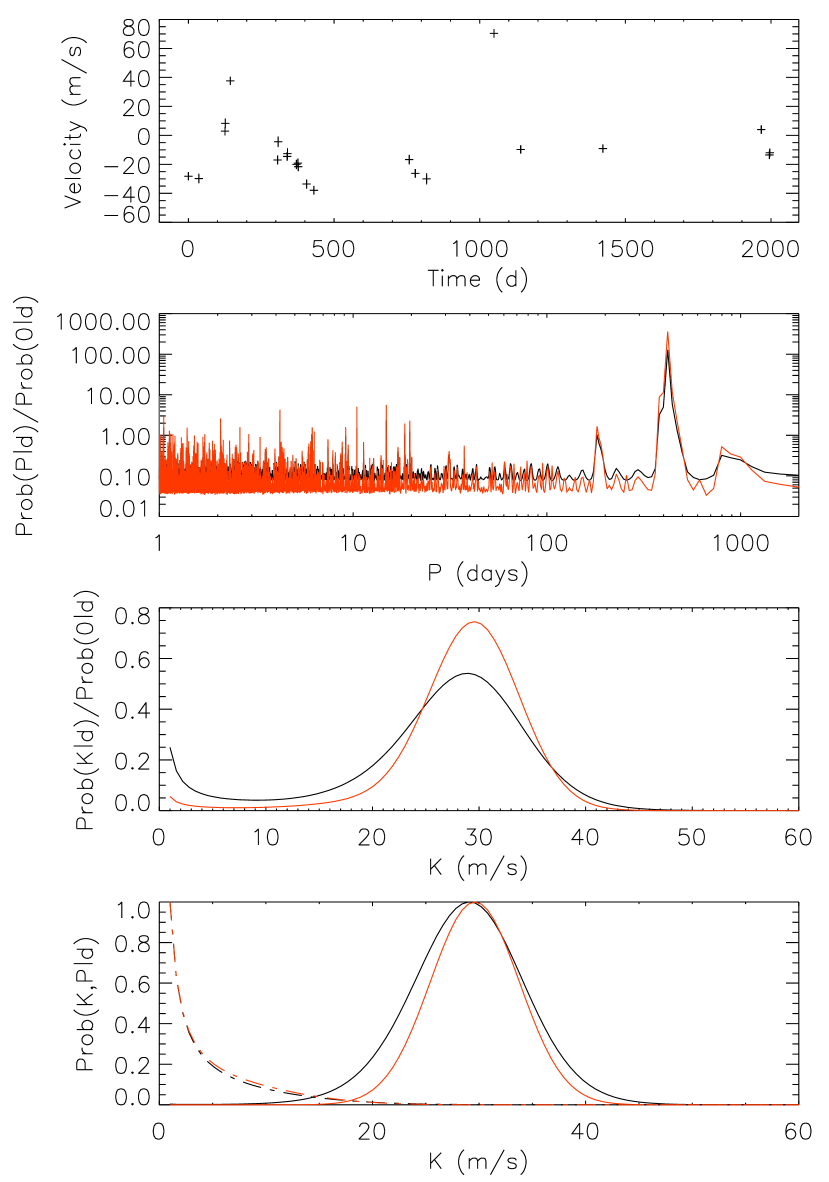
Figure 1: Results of circular orbit fitting to data for HD 4203, using analytic marginalization over $K$ and $\phi$, and reconstructing ${\mathcal{P}}(K)$ using equation (38) (red curves) and by calculating ${\mathcal{P}}(\phi,K,P)$ on a grid (black curves). ${\mathcal{P}}(K)$ in the third panel is normalized such that each curve has the same area beneath the curve. The bottom panel compares the ${\mathcal{P}}(K)$ obtained for periods $420.1$ days (solid curves, close to the best-fitting frequency) and $19.0$ days (dot-dashed curves, no significant fit at this frequency) for the analytic and grid-based approaches.

3.5 Summary and example

Let’s summarize the main results of this section. We have discussed two methods for evaluating ${\mathcal{P}}(P,K|d)$ for circular orbits. First, equations (3.2) and (22) can be used to calculate $\chi^{2}(P,K,\phi)$ for many different values of $P$, $K$, and $\phi$, and from there ${\mathcal{P}}(P,K|d)$ obtained by integration over $\phi$. No approximations are made in this approach, which we refer to as the “grid-based approach”. Second, equations (27) to (33) provide a method for evaluating ${\mathcal{P}}(P|d)$ using analytic marginalization over the linear parameters $A$ and $B$ and therefore $K$ and $\phi$. The analytic marginalization requires that we assume a prior ${\mathcal{P}}(K)\propto K$ rather than $1/K$, but by choosing the normalization appropriately (eq. [33]), we approximately recover the results corresponding to ${\mathcal{P}}(K)\propto 1/K$. Next, given the best fit amplitude $K_{0}=(A_{0}^{2}+B_{0}^{2})^{1/2}$ at each period, ${\mathcal{P}}(P,K|d)$ can be calculated for a grid of $K$ values using the analytic approximation of equation (38). We refer to this second approach as the “analytic approach”.

As an example, we consider the 23 radial velocities for the star HD 4203 made available in the Butler et al. (2006) catalog of nearby exoplanets (see Vogt et al. 2004 for the original discovery of this planet). The orbital parameters given by Butler et al. (2006) are $P=431.88\pm 0.85$ days, $K=60.3\pm 2.2\ {\rm m/s}$, and $e=0.519\pm 0.027$. They also include a linear long term trend of $-4.38\pm 0.71\ {\rm m\ s^{-1}\ yr^{-1}}$. The rms of the residuals to this solution is $4.1\ {\rm m/s}$.

We use both of the techniques described above to fit a circular orbit plus constant to this data. We consider orbital periods between 1 day and the time-span of the data, $T=2000$ days. We evaluate $4N_{f}$ frequencies, where $N_{f}=(\Delta f)T$ is the estimated number of independent frequencies in the frequency range $\Delta f$ (Cumming, 2004). The values of $K$ considered range from $1\ {\rm m/s}$ to $2\Delta v$, where $\Delta v$ is the range of the measured velocities. For the grid-based approach, we find that the typical time required on a 2–3 GHz CPU is $\sim 10^{-7}\ {\rm s}$ per set of parameters $(\phi,K,P)$, so that for example 3000 periods, 100 values of $K$ and $30$ phases, or $10^{7}$ total combinations, takes $1\ {\rm s}$ to evaluate. For $\phi$, we align the grid with the best fit phase $\phi_{0}$ at each $P$. In this way, we guarantee that the best fit value of $\phi$ is included on the grid, which reduces the number of grid points we need to use in $\phi$. The analytic marginalization technique requires $\sim 5\times 10^{-7}\ {\rm s}$ per $P$ and $K$ value, so that a search of 3000 periods, keeping track of 100 values of $K$ takes $\sim 0.1\ {\rm s}$. We use the routine bessi0 from Press et al. (1992) to calculate the Bessel function in equation (38).

Figure 1 compares the two techniques. The red curves show the results of the analytic marginalization, the black curves show the results of the grid-based calculation. The false alarm probabilities are $0.14$ (grid) and $0.060$ (analytic) (odds ratios $6.3$ and $16$ respectively). The distribution of $K$ agrees well between the two techniques, although the probability curve is shifted to larger values of $K$ for the analytic approach compared to the grid approach, consistent with the different priors. The false alarm probability $\sim 0.1$ means that this would not count as a detection. This is an example of a case in which the large eccentricity $e>0.5$ prevents detection by fitting circular orbits. The best fit amplitude $K\approx 30\ {\rm m/s}$ for circular orbits is significantly smaller than for the Keplerian orbit fit of Butler et al. (2006). Using 100 values of $K$ between $1\ {\rm m/s}$ and $60\ {\rm m/s}$, we find the 99% upper limit on $K$ is $41.2\ {\rm m/s}$ (analytic) or $41.3\ {\rm m/s}$ (grid). The bottom panel in Figure 1 compares the probability distribution of $K$ at two different periods obtained from the grid-based approach and the analytic approach. This shows that equation (38) reproduces the distribution from the grid-based calculation well.

4 Eccentric orbits

We now consider full Keplerian fits to the data. The techniques we developed in the previous section for circular orbits can be readily applied to Keplerian orbits, because the Keplerian model is linear in a subset of parameters which can therefore be treated analytically, as we now describe.

4.1 Calculation of ${\mathcal{P}}(P,K,e|d)$

For a Keplerian orbit, the radial velocity can be written

$$V=\gamma+K\left[\cos(\theta+\omega_{p})+e\cos\omega_{p}\right]$$ (39)

where $K$ is the velocity amplitude, $e$ is the eccentricity of the orbit, $\omega_{p}$ is the argument of periastron. The true anomaly $\theta$ is a function of the time $t$ and the three parameters $e$, $P$, and $t_{p}$, where $t_{p}$ is the time of periastron passage (acting as an overall phase for $V(t)$). To calculate $\theta(t;e,P,t_{p})$, we must solve the relations

$$\tan\left({\theta\over 2}\right)=\left({1+e\over 1-e}\right)^{1/2}\tan\left({E\over 2}\right)$$ (40)

$$E-e\sin E=M={2\pi\over P}(t-t_{P})$$ (41)

where $E$ is the eccentric anomaly, and $M$ the mean anomaly.

The first point to note is that the six orbital parameters, $\vec{a}=(\gamma,K,\omega_{p},P,e,t_{p})$ can be divided into two groups, “slow” and “fast” parameters, $\vec{a_{s}}=(P,e,t_{p})$ and $\vec{a_{f}}=(\gamma,K,\omega_{p})$ respectively. Each time we change a value of the slow parameters, we must re-solve equations (40) and (41) to calculate the values of $\theta$, whereas when we change a value of the fast parameters only we do not need to recalculate the values of $\theta$. This is reminiscent of the division into fast and slow parameters in analysis of CMB data (e.g. Lewis & Bridle 2002; Tegmark et al. 2004). We can use this division to increase the speed of the parameter search.

For a given set of the slow parameters, we can find the best fitting fast parameters with a linear least-squares fit, since we can write

$$V=A\sin\theta+B\cos\theta+\tilde{\gamma}$$ (42)

with $A=-K\sin\omega_{p}$, $B=K\cos\omega_{p}$, and $\tilde{\gamma}=\gamma+Ke\cos\omega_{p}$. A linear least-squares fit returns the best-fitting values of $A$,$B$, and $\tilde{\gamma}$, and therefore $K$ ($K^{2}=A^{2}+B^{2}$), $\omega_{p}$ ($\tan\omega_{p}=-B/A$), and $\gamma$. This halves the number of parameters that we need to search to find the best-fitting solution.

The fact that the fast parameters $\vec{a_{f}}$ can be obtained from a linear fit means that we can directly apply the techniques we developed for circular orbits in §3 to marginalize over them. For the grid-based approach, equation (3.2) should be replaced by

$${\chi^{2}(K,\omega_{p})\over\sum w_{i}}=\langle\langle v^{2}\rangle\rangle+2K\left[\langle\langle vS\rangle\rangle\sin\omega_{p}-\langle\langle vC\rangle\rangle\cos\omega_{p}\right]$$

$$+K^{2}\left[\langle\langle C^{2}\rangle\rangle\cos^{2}\omega_{p}+\langle\langle S^{2}\rangle\rangle\sin^{2}\omega_{p}\right.$$

$$\left.-\langle\langle SC\rangle\rangle 2\sin\omega_{p}\cos\omega_{p}\right]$$ (43)

where $\omega_{p}$ now plays the same role as $\phi$ for circular orbits, and the sums over the data involve $\theta_{i}$ rather than $\omega t_{i}$. For example, the definition of $\langle S\rangle$ in equation (3.2) should be replaced by $\langle S\rangle=\sum w_{i}\sin\theta_{i}/\sum w_{i}$.

Similarly, since equations (24) and (42) are of the same form, the analytic integration over $A$ and $B$ can be applied directly to the Keplerian case, giving ${\mathcal{P}}(P,e,t_{p}|d)$ analytically from equations (27) to (33). As for circular orbits, the distribution of velocity amplitude at each $(P,e,t_{p})$, ${\mathcal{P}}(K,P,e,t_{p}|d)$, can be recovered, being well-approximated by equation (38).

Figure 2: Results of Keplerian fits to the HD 4203 data from Butler et al. 2006, including a linear trend. In this coarse scan of parameter space, ${\mathcal{P}}(P,e,K|d)$ is calculated for 10 eccentricities between 0 and 0.9, 10 velocities between 1 and $217\ {\rm m/s}$ (twice the velocity span of the data), and 7978 periods between 1 day and 1996 days (the time span of the data).

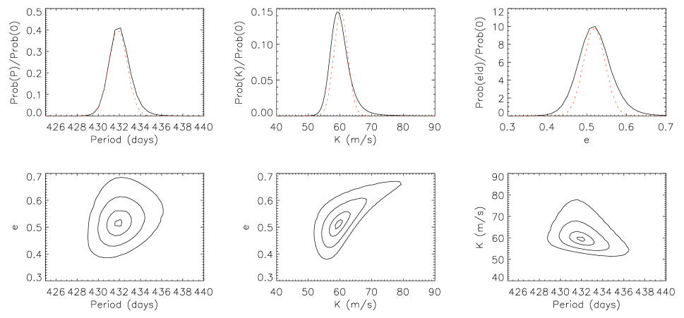
Figure 3: Results of Keplerian fits to the HD 4203 data from Butler et al. 2006, including a long term trend. The dotted curves show Gaussian distributions with central values and standard deviations matching those given by Butler et al. 2006. 100 values of K, 30 eccentricities and 30 periods were calculated in the range shown. The contours enclose 10%, 50%, 90% and 99% of the probability.

4.2 Example

As an example, we return to the HD 4203 data considered previously. We first calculate ${\mathcal{P}}(P,e|d)$ for a grid in $P$ and $e$. The integration over $t_{p}$ is carried out using a simple algorithm in which we double the number of equally-spaced $t_{p}$ values until the required accuracy is obtained. For each combination of $P$, $e$, and $t_{p}$ considered, we analytically integrate over $\gamma$, $K$, and $\omega_{p}$, and at the same time use equation (38) to keep track of ${\mathcal{P}}(K;P,e,t_{p}|d)$. We use Newton’s method to solve Kepler’s equation, taking advantage of the fact that the required derivative can be calculated analytically. Our implementation of this algorithm takes $\approx 5\times 10^{-5}\ {\rm s}$ per $P$, $e$, and $t_{p}$ value considered, with 30 $K$ values tracked through the calculation. For an average 200 values of $t_{p}$, 10 eccentricities, and 3000 periods, the total time needed is $\approx 30\ {\rm s}$ for a scan of parameter space. We have also implemented the grid-based approach, and find that it is about 10 times slower than the analytic approach. The results agree well between both techniques.

The results for HD 4203 are shown in Figures 2 and 3. We first run a coarse scan of the parameter space for a single Keplerian orbit plus a linear trend. We calculate $4N_{f}\approx 8000$ frequencies, corresponding to the period range $1$ day to $\approx 2000$ days (the time span of the data), 10 eccentricities between 0 and 0.9, 10 velocities between $1\ {\rm m/s}$ and $216\ {\rm m/s}$ (twice the velocity span of the data). The resulting constraints on $P$, $e$ and $K$ are shown in Figure 2. The odds ratio is $4\times 10^{4}$ for the Keplerian orbit plus linear trend compared to a constant velocity model. We show the results including a linear trend, because the best fit model presented by Butler et al. (2006) includes a trend, but in fact our results at this stage do not require a trend. The odds ratio for a similar search but without the linear term is $5\times 10^{4}$.

We then carry out a more detailed calculation of the parameter space near the best fitting model corresponding to the peak in ${\mathcal{P}}(P|d)$ at $\approx 440$ days in Figure 2. The results are shown in Figure 3. The odds ratio is $9.5\times 10^{10}$ for a Keplerian orbit plus trend compared to a constant model (for the ranges of parameters shown in Fig. 3). The much larger value of the odds ratio compared to our coarse calculation is because the parameter space considered is smaller and the peak in ${\mathcal{P}}(P,e,K|d)$ has now been resolved. We can renormalize the odds ratio to correspond to the full range of parameter space considered in the coarse search by multiplying by the ratio of $\log P_{2}/P_{1}$ and $\log K_{2}/K_{1}$ in each calculation. Doing this, we find an odds ratio $7.4\times 10^{7}$. Without the linear trend the odds ratio is 100 times smaller, $7\times 10^{5}$, normalized to the full range of parameters. This indicates that a model with a linear trend is strongly preferred given this data. Without the linear trend, the probability peaks at similar values of $P$ and $K$, but with a larger eccentricity, $e\approx 0.7$.

The dotted curves in Figure 3 show Gaussian distributions with the central values and standard deviations given by Butler et al. (2006) for $K$, $P$, and $e$. Overall there is good agreement with the central values and widths.

Repeating the calculation shown in Figure 3 with the grid-based method for marginalizing over $K$ and $\omega_{p}$ gives almost identical constraints on orbital parameters, but a smaller odds ratio by a factor of two, $3.5\times 10^{7}$ compared to $7.4\times 10^{7}$. We have also checked that other peaks in ${\mathcal{P}}(P|d)$ that can be seen in Figure 2 do not contribute significantly to the odds ratio. The next most important is the peak at $P\approx 800$ days, but its odds ratio is 400 times smaller than the peak at 432 days shown in detail in Figure 3.

The coarse sampling for HD 4203 gave an odds ratio that was a factor of 400 smaller than the final odds ratio obtained by zooming in on the most significant peak. We find that increasing the period sampling by a factor of two to $8T\Delta f$ gives an odds ratio from the coarse search in good agreement with the odds ratio from zooming in on the peak.

5 Comparison with previous work

In §4, we presented an algorithm that can efficiently compute ${\mathcal{P}}(P,K,e|d)$ for a radial velocity data set. As described in §2, this contains information about the constraints on $P$, $K$, and $e$ and also allows a false alarm probability to be calculated. We now use our algorithm to recalculate results in the literature from MCMC and other techniques and compare.

Figure 4: The eccentricity distribution derived for HD 76700, using data from Tinney et al. 2003. The solid curve is for analytical marginalization over the noise scaling parameter $k$, the dotted curve is for $k=1$, and the dashed curve shows $e{\mathcal{P}}(e|d)$, corresponding to a uniform prior in $d(e\cos\omega_{p})d(e\sin\omega_{p})$.

5.1 Orbital parameter constraints from MCMC calculations

Ford (2005) used a MCMC calculation to study the constraints on orbital parameters from radial velocity data, and this paper has been followed by several others (Ford, 2006, 2008; Ford & Gregory, 2007; Gregory, 2005b, 2007a, 2007b; Balan & Lahav, 2009). We have calculated the constraints on orbital parameters for the different single planet cases considered in these papers, and overall the agreement is excellent.

One difference is that in several published cases, the posterior probability for eccentricity drops towards zero at low eccentricities, whereas we find ${\mathcal{P}}(e|d)$ is approximately constant as $e$ goes to zero. For HD 76700, this difference appears to be because of the different prior assumed by Ford (2005). The MCMC calculations in that paper take steps in $e\cos\omega_{p}$ and $e\sin\omega_{p}$ in such a way that the assumed prior is uniform in $d(e\cos\omega_{p})d(e\sin\omega_{p})$ giving a prior $e\,de\,d\omega_{p}\propto e$. In Figure 4, we allow for this different prior by plotting $e{\mathcal{P}}(e|d)$, and the result compares favorably with Figure 2 of Ford (2005). (Ford 2005 discusses the use of importance sampling, in which the samples are weighted $\propto 1/e$ to give an effective prior uniform in $e$, but this does not seem to have been applied in Figure 2 of that paper).

For HD 72659, marginalization over the extra noise source opens up considerable parameter space at low eccentricity. In Figure 5, we show the constraints on eccentricity and period with $k$ fixed at $k=1$ and with $k$ marginalized over. Ford (2005), unlike later papers (e.g. Ford 2006) does not include an additional noise term, and our results for $k=1$ compare well with Figures 4 and 5 of that paper.

Figure 5: The eccentricity distribution and joint eccentricity-orbital period distribution derived for HD 72659. The top panels are for analytic marginalization over the noise parameter $k$, whereas the bottom panels take $k=1$ as in Ford 2005. Contours enclose 10, 50, 90 and 99% of the probability.

5.2 Odds ratios from Gregory’s parallel tempering MCMC approach

In a series of papers, Gregory has developed a MCMC code which uses parallel tempering to exchange information between chains running with different “temperatures”. Combining the results of different chains gives the total posterior probability for the model, allowing calculations of odds ratios and therefore model comparisons.

Gregory (2005b) analyzed 18 radial velocities for HD 73526 from Tinney et al. (2003). The period range was from 0.5 days to 3732 days, and velocities from 0 to $400\ {\rm m/s}$ using a Jeffrey’s prior with a break at $1\ {\rm m/s}$. An additional noise term was added which was allowed to range between $0$ and $100\ {\rm m/s}$. He pointed out that there were two additional possible solutions with $P\approx 128$ and $376$ days besides the previously obtained solution at $P\approx 191$ days. A chain covering the entire parameter space did not converge, and so separate chains were run focussing on each of the three probability peaks. The odds ratio for a planet compared to a constant velocity was found to be $9.3\times 10^{5}$ (Table 5 of Gregory 2005b). We ran a calculation with the same period and velocity range as Gregory (2005b) (except that we take the lower bound in $K$ to be $1\ {\rm m/s}$ with a Jeffrey’s prior) ($9940$ frequencies, 30 eccentricities and 30 velocities). The odds ratio was $3.3\times 10^{6}$. Zooming in on the three peaks gives probability distributions for $e$, $P$, and $K$ that are very similar to the results of Gregory (2005b). The odds ratios for the $P\approx 128$, $190$, and $376$ day peaks are $2.4\times 10^{4}$, $1.1\times 10^{5}$, and $1.0\times 10^{6}$ (assuming the full prior range so that these numbers can be compared). The sum of these, $1.1\times 10^{6}$ agrees well with the odds ratio found by Gregory (2005b) whose odds ratio includes only these three peaks. The relative probabilities of the three peaks are 2%, 10% and 88%. Gregory (2005b) found relative probabilities of 4%, 3% and 93%.

Gregory (2007a) found evidence for a second planet in HD 208487; we compare to their odds ratio and posterior probability for a one-planet fit. The posterior probability distributions were calculated for the 35 velocities from Butler et al. (2006). We find excellent agreement with the distributions of $P$, $e$ and $K$ shown in Figure 7 of Gregory (2007a). The odds ratio for a single planet model for this data (Table 6 of Gregory 2007a) was $1.7$–$2.6\times 10^{4}$ for two different choices of the turnover in the modified Jeffrey’s prior for the extra noise scale. For the parameter ranges in Figure 7 of Gregory (2007a), we find an odds ratio of $1.4\times 10^{8}$. Rescaling to a velocity range $1$–$2129\ {\rm m/s}$, and period range $1$ day to 1000 years, this becomes $6.1\times 10^{4}$, a factor of 3 times greater than Gregory (2007a). (The details of the priors were different, for example, the upper limit on velocity in Gregory 2007a’s prior depended on period and eccentricity, but we expect this to give only a small difference).

Gregory (2007b) presented evidence for three planets in HD 11964 from 87 radial velocities in the Butler et al. (2006) catalog. The odds ratio reported for the single planet model is $3\times 10^{9}$ (Table 4 of Gregory 2007b). We find an odds ratio in good agreement, $2\times 10^{9}$. Although Gregory (2007b) does not show posterior probability distributions for orbital parameters for the one planet model, the distributions of $P$, $e$ and $K$ we find compare well with those for the $P\approx 2000$ day signal in the three planet model of Gregory (2007b). For this data, Butler et al. (2006) include a linear term. We find the odds ratio for a linear versus constant no-planet model to be 1300. Including a linear term in the planet model gives an odds ratio of $3\times 10^{6}$, much smaller than the odds ratio for a planet model only. Therefore, we find that a single planet model with $P\approx 2000$ is preferred over a linear trend only or planet plus linear trend by a large factor (in agreement with Wright et al. 2007 who also concluded that the trend reported by Butler et al. 2006 was likely spurious).

5.3 False alarm probabilities

Marcy et al. (2005) discuss the calculation of false alarm probabilities using a scrambled velocity method in which the residuals to the best-fitting Keplerian orbit are used as an estimate of the noise distribution. In that paper, they announced five new planets from the Keck Planet Search. False alarm probabilities were calculated for two cases that looked marginal, HD 45350 (FAP$<0.1$% scrambled, $4\times 10^{-5}$ F-test) and HD 99492 (FAP$\approx 0.1$% scrambled, $3\times 10^{-4}$ F-test). For HD 99492, we find odds ratios scaled to 1.0 for no planet are 0.33 for a linear trend but no planet, 1.66 for a planet, 200.0 for a planet plus linear trend. Therefore, a linear trend is preferred in this case. The FAP using equation (13) for the odds ratio is $7\times 10^{-3}$. For HD 45350, we find odds ratios: 1.0, 0.18, $6.7\times 10^{5}$, $4.7\times 10^{5}$, giving FAP$\approx 10^{-6}$. As Marcy et al. (2005) noted, the evidence for a linear trend in this source is marginal (the odds ratios are similar with and without a trend).

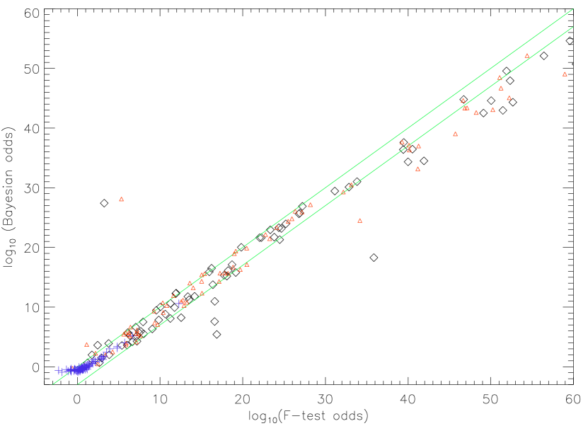
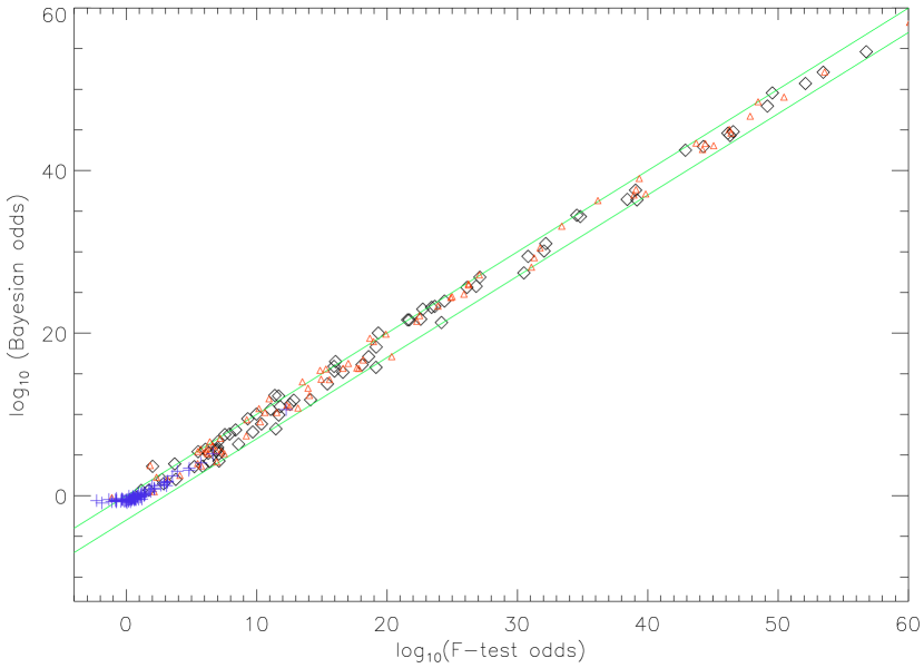
Figure 6: Comparison between logarithm of the odds ratio $\log_{10}\Lambda$ from the Bayesian calculation and the F-test. The Bayesian odds ratios are from coarse sampling ($8T\Delta f$ periods, 10 eccentricities) of the 84 radial velocity data sets from Keck, Lick, and AAT published as part of the Butler et al. 2006 catalog. We compare with analytic F-test FAPs, converted to odds ratios using the relation $\Lambda=(1/F)-1$. The crosses are the odds ratios for a linear trend versus constant velocity, the diamonds are odds ratios for a planet versus constant, and the triangles are for planet plus long term trend versus long term trend only. The upper panel uses a Keplerian fitting routine to determine the F-test FAP, whereas in the lower panel we use the minimum $\chi^{2}$ found in the Bayesian routine to calculate the analytic FAP.

Cumming (2004) described a quick estimate of the FAP based on an F-test at each independent frequency. Generalizing the Lomb-Scargle periodogram to eccentric orbits, the idea is to define a power at each frequency

$$z={(N-5)\Delta\chi^{2}\over 4\chi^{2}_{\rm Kep}}={(N-5)(\chi^{2}_{0}-\chi^{2}_{\rm Kep})\over 4\chi^{2}_{\rm Kep}}.$$ (44)

For Gaussian noise, $z$ follows the $F_{4,N-5}$ distribution, which allows a calculation of ${\rm Prob}(z>z_{\rm max})$ for an observed maximum power $z_{\rm max}$. The FAP is then

$${\rm FAP}=1-(1-{\rm Prob}(z>z_{\rm max}))^{N_{f}}\approx N_{f}{\rm Prob}(z>z_{\rm max}).$$ (45)

The number of independent frequencies $N_{f}$ can be estimated as $N_{f}\approx T\Delta f$.

We have used this approach to calculate the FAP for the 84 stars with published radial velocities as part of the Butler et al. (2006) catalog of exoplanets. To find $\chi^{2}_{\rm Kep}$, we follow the automated procedure used by Cumming et al. (2008), which involves using the top two well-separated peaks in the Lomb-Scargle periodogram as starting periods for full Keplerian fits. To compare with the Bayesian odds ratios, we convert the F-test FAP into an odds ratio by inverting equation (9). To find Bayesian odds ratios, we run a coarse sampling of the parameter space with $8T\Delta f$ periods for each of these 84 stars, with and without a long term linear trend.

The results are shown in Figure 6. In the lower panel, we use the minimum value of $\chi^{2}$ found in the Bayesian calculation to calculate the F-test FAP. In this case, the odds ratios are well-correlated, although with the Bayesian odds ratio between 1 and 1000 times smaller than the F-test odds ratio. In the upper panel, there is more scatter. This arises from differences between the minimum $\chi^{2}$ values found by the Keplerian fitting routine and the Bayesian routine. For example, the two points above and to the left of the upper panel of Figure 6 are for HD 80606, which has a very eccentric orbit. Our Keplerian fitting routine, which uses circular orbit fits as its starting point failed to find the best-fitting solution, whereas the Bayesian routine, with its systematic scan of parameter space did find it. Generally the scatter is downwards, indicating that the Bayesian routine sometimes find a larger minimum $\chi^{2}$ than the Keplerian fitting routine. Likely this is due to the finite period sampling, whereas the Keplerian fitting routine can adjust the period to lower $\chi^{2}$.

The fact that the Bayesian odds ratios tend to be lower than the F-test odds ratios indicates that the Bayesian calculation is more conservative than the F-test. In fact, this is expected. Cumming (2004) showed that the Bayesian odds ratio is closely related to the F-test (periodogram), but with a different definition for the number of independent frequencies. In the Bayesian calculation, the number of trials counts the frequencies, but also the range of the other parameters (Cumming, 2004). In this way, the Bayesian calculation penalizes models with larger ranges of parameters, for all parameters, not just frequency.

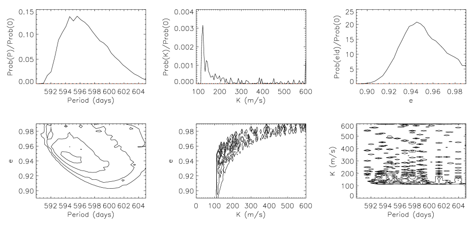
Figure 7: Results of Keplerian fits to the HD 20782 data from O’Toole et al. 2008. 30 eccentricities, 30 periods and 100 $K$ values were calculated in the ranges shown. Contours enclose 10%, 50%, 90%, and 99% of the total probability.

Figure 8: Results of Keplerian fits to the 5319 data including a linear trend. 30 eccentricities, 30 periods and 100 $K$ values were calculated in the ranges shown. Dotted curves show Gaussian distributions with central values and standard deviations taken from Robinson et al. 2007. Contours enclose 10%, 50%, 90%, and 99% of the total probability.

5.4 2D periodograms

Wright et al. (2007) investigate the constraints that can be placed on the orbital parameters of long period orbits that have been only partially observed. They calculated the minimum $\chi^{2}$ at points across the $m\sin i$-$P$ plane. Similarly, O’Toole et al. (2008) introduced a “2D Keplerian Lomb-Scargle periodogram” (2DKLS) in which the periodogram power is evaluated on a grid of $P$ and $e$, with a full Keplerian fit carried out at each point. O’Toole et al. (2008) discuss the considerable computing resources being used to conduct simulations of detectability using this new 2D periodogram. The techniques we discuss earlier for rapid evaluation of multiple $\chi^{2}$ values could prove useful in more efficiently evaluating the 2DKLS periodogram. The constraints on $P$-$e$ or $P$-$K$ calculated in this paper differ from Wright et al. (2007) and O’Toole et al. (2008) in that for each choice of $P$, $e$ or $P$, $K$ all values of the other parameters are taken into account, weighted by their probability, rather than finding the best fit values of the other parameters. This is the standard difference between Bayesian and frequentist approaches.

O’Toole et al. (2008) mention that one of the reasons for looking at the periodogram power as a function of $P$ and $e$ is to help with detection of highly eccentric orbits. They consider the $e=0.97$ planet around HD20782 as an example. Their best fit has $e=0.97\pm 0.01$, $P=591.9\pm 2.8$, and $K=185.3\pm 49.7$. Our results for this data are shown in Figure 7. The discrete nature of the $K$ distribution is due to the finite sampling of the grid in eccentricity. The O’Toole et al. (2008) solution lies on our contours, but towards the edge. The Bayesian calculation, which averages over the marginalized parameters, opens up a wider parameter space than the best-fit and error bars from O’Toole et al. (2008) suggest.

5.5 HD 5319

HD 5319 has a planet with minimum mass $1.9\ M_{J}$ in a 675 day low eccentricity orbit (Robinson et al., 2007). This is an interesting example to compare to because the analysis of Robinson et al. (2007) used several different statistical methods. First, they used Monte Carlo simulations of data sets with noise only (simulated by selecting with replacement from the observed velocities) to assess the FAP, finding $1.3\times 10^{-3}$. They used both a scrambled velocity Monte Carlo simulations and an MCMC Bayesian calculation to estimate the uncertainties in the derived orbital parameters. They used an F-test to test the significance of including a linear trend in their model, finding a FAP of $3\times 10^{-4}$ indicating that a linear term is strongly preferred.

The results of our calculation are shown in Figure 8. The dotted lines show the best fitting parameters and the errors found by Robinson et al. (2007), assuming Gaussian distributions, and agree well both in terms of central values and widths. Interestingly, the MCMC simulations run by Robinson et al. (2007) did not agree as well with their scrambled velocity approach, whereas we find good agreement. The odds ratio for a trend in the no planet model is 0.9. For models with a planet, the odds ratios are $9.0\times 10^{8}$ (with trend) and $1.0\times 10^{6}$ (without trend). The model with a trend therefore has greater odds by a factor of $10^{3}$, in good agreement with the F-test FAP of $3\times 10^{-4}$ found by Robinson et al. (2007). However, the overall false alarm probability we find $\sim 10^{-9}$ is much smaller than the simulations of Robinson et al. (2007) suggested, $\sim 10^{-3}$.

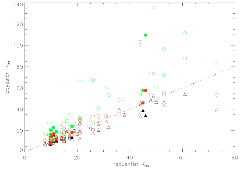
Figure 9: Comparison between the 99% upper limits on $K$ for circular orbits determined by Cumming et al. 1999 for 63 stars from the Lick Planet Search, and the 99% upper limits on $K$ from a Bayesian analysis of the same data. Solid triangles or circles include a linear trend in the fits (these are the 7 stars that Cumming et al. 1999 found to have a significant slope), whereas open triangles or circles do not include a linear trend. The dotted line indicates a 1:1 correspondence between the two calculations of the upper limit. The black triangles are for circular orbits, the red circles are for eccentric orbits with $e<0.5$ and the green circles are for eccentric orbits with $e<0.7$.

5.6 Upper limits on $K$

In an analysis of the Lick Planet Search, Cumming et al. (1999) calculated upper limits for 63 stars with non-detections. They used a Monte Carlo approach, in which simulated data sets with a circular orbit plus noise were analyzed and the velocity amplitude determined which resulted in detection 99% of the time. We have reanalyzed the same data using our Bayesian scheme, first with circular orbits, and then with eccentric orbits. We calculate the 99% upper limit $K_{99}$ by $\int_{0}^{K_{99}}\ dK\ {\mathcal{P}}(K|d)=0.99$ (where ${\mathcal{P}}(K|d)$ is normalized so that the total probability is unity).

The results are shown in Figure 9. The triangles are for circular orbit models, and the circles are for eccentric orbits. For the 7 stars found to have a significant linear trend by Cumming et al. (1999), we include a linear trend in the model. Overall the agreement is good. Cumming et al. (1999) (and Cumming et al. 2008) calculate upper limits for circular orbits to reduce the computational time needed. Based on the calculations of the effect of eccentricity on detectability of Endl et al. (2002) and Cumming (2004), they proposed that $K_{99}$ for circular orbits would be a good estimate of $K_{99}$ for orbits with $e\la 0.5$. We can test that here by calculating $K_{99}$ from the partial $K$ distribution

$${\mathcal{P}}(K|d)=\int^{e_{\rm cutoff}}_{0}\ de\ {\mathcal{P}}(e,K|d)$$ (46)

with different cutoffs $e_{\rm cutoff}$. For $e_{\rm cutoff}=0.9$, we find that the value of $K_{99}$ is generally much greater than $K_{99}$ for circular orbits, due to a tail of large $K$, large eccentricity solutions. However, for $e_{\rm cutoff}=0.5$, the agreement is very good. This is shown in Figure 9, where we show results for $e_{\rm cutoff}=0.5$ (red symbols) and $e_{\rm cutoff}=0.7$ (green symbols). The $e_{\rm cutoff}=0.7$ values of $K_{99}$ are significantly greater than the circular orbit or $e_{\rm cutoff}=0.5$ values.

6 Summary and Conclusions

In this paper, we consider Bayesian analysis of radial velocity data. An advantage of this kind of analysis over traditional methods is that a single calculation gives the false alarm probability and the probability distributions of orbital period, eccentricity and velocity amplitude, allowing error bars or upper limits on these quantities to be determined. Using periodogram methods, separate calculations are required for each of these quantities, typically requiring many Monte Carlo trials.

Previous work on Bayesian analysis of radial velocities has used Markov Chain Monte Carlo (MCMC) techniques (although see Ford 2008 who used analytic techniques to partially carry out the marginalization for circular orbits). Our approach has been to apply some exact and approximate analytic results (based on previous work by Jaynes 1987 and Bretthorst 1988) to the marginalization integrals for Keplerian fits to radial velocity data. In particular, we analytically integrate over the linear model parameters for each combination of $P$, $e$, and $t_{p}$, and use an analytic approximation (eq. [38]) to reconstruct the probability distribution of $K$. An implementation of this algorithm in IDL is available on request from the authors.

With this approach, a full search of parameter space for a single Keplerian orbit takes several minutes on a $2$–$3\ {\rm GHz}$ processor, or several seconds for circular orbits, making it applicable to data sets from large velocity surveys. Constraints on orbital parameters (which involve surveying smaller regions of parameter space) can be calculated in seconds, competitive with MCMC techniques. Our calculation can certainly be improved further. For example, we have focussed on the marginalization over the linear parameters in this paper, and used the simplest approach of evaluation on an evenly-spaced grid to integrate over the remaining parameters $P$, $K$, and $e$.

We compared our results with previous calculations. The constraints on orbital parameters and odds ratios agree well with MCMC results. We find that the Bayesian odds ratios are systematically lower than F-test odds ratios by a factor between 1 and 1000. This is due to the different accounting of trials in the two calculations (Cumming, 2004), with the Bayesian calculation including an Occam’s razor penalty which accounts for the range of all parameters rather than only the frequency range. The techniques we have developed for rapidly calculating $\chi^{2}$ may have application to other techniques, such as the 2D periodograms of Wright et al. (2007) and O’Toole et al. (2008). We find good agreement with the upper limits on velocity amplitude $K$ calculated for circular orbits by Cumming et al. (1999) if we restrict our attention to $e\la 0.5$. More eccentric orbits give rise to a tail of solutions at large $K$. This shows that characterizing the $K$ distribution with a single parameter (e.g. the 99% upper limit; Cumming et al. 2008) is not appropriate for population analyses with highly eccentric orbits included. On the other hand, for low to moderate eccentricity orbits ($e\la 0.5$), upper limits can be derived from circular orbit fits which is much less numerically intensive.

The division of Keplerian parameters into “fast” and “slow” may prove useful in MCMC simulations. At the least, the systemic velocity does not need to be included as a parameter; it can be quickly evaluated for each set of the other parameters, and used to evaluate $\chi^{2}$ (this was also noted by Ford 2006). One possible complication is that Ford (2005) takes steps in a mixture of fast and slow parameters, $e\cos\omega$ and $e\sin\omega$, to help speed convergence. Separating the slow and fast parameters could potentially reduce efficiency in this case. Further investigations are needed.

Appendix A Including a linear term (long term trend)

In the main text, the “no planet” model that we have compared the sinusoid and Kepler fits to was a constant velocity model. Often, a linear term is included in the fit to account for long timescale trends in the data. Since adding a linear trend adds one extra linear term to the model, we can analytically marginalize over the slope in the same way as we marginalize over the constant term. In this Appendix, we give the formulae to do that.

A.1 Is there evidence for a long term trend?

First, consider a constant versus a linear model. Minimizing $\chi^{2}$ as a function of $\gamma$ for $V_{i}=\gamma$, we find the best fit constant term is

$$\gamma_{0}=\langle v\rangle,$$ (47)

the corresponding minimum value of $\chi^{2}$ is

$${\chi^{2}_{\rm const}\over\sum w_{i}}=\langle\langle v^{2}\rangle\rangle,$$ (48)

and

$$\det\alpha=\sum w_{i}.$$ (49)

Inserting these expressions into equation (26) with the number of parameters $m=1$ gives the posterior probability for a fit of a constant.

For a straight line fit, $V_{i}=\gamma+\beta t_{i}$, we find

$$\gamma_{0} = {\langle v\rangle\langle t^{2}\rangle-\langle vt\rangle\langle t\rangle\over\langle\langle t^{2}\rangle\rangle}$$ (50)

$$\beta_{0} = {\langle\langle vt\rangle\rangle\over\langle\langle t^{2}\rangle\rangle}$$ (51)

$${\det\alpha\over(\sum w_{i})^{2}} = \langle\langle t^{2}\rangle\rangle$$ (52)

$${\chi^{2}_{\rm line}\over\sum w_{i}} = \langle v^{2}\rangle-2\gamma_{0}\langle v\rangle-2\beta_{0}\langle vt\rangle$$ (53)

$$+\gamma_{0}^{2}+2m\beta_{0}\gamma_{0}\langle t\rangle+\beta_{0}^{2}\langle t^{2}\rangle$$

Using equation (26), the odds ratio is

$$\Lambda={(\chi^{2}_{\rm line})^{-(N-2)/2}\over(\chi^{2}_{\rm const})^{-(N-1)/2}}\left({\pi\over(\sum w_{i})\langle\langle t^{2}\rangle\rangle}\right)^{1/2}$$

$${\Gamma((N-2)/2)\over\Gamma((N-1)/2)}{1\over\Delta\beta},$$ (54)

where $\Delta\beta$ is the prior range for $\beta$ (the prior range for $\gamma$ is the same in both models, and cancels). Here, we take $\beta$ to lie between $\pm\Delta v/T=\pm(v_{\rm max}-v_{\rm min})/T$, giving $\Delta\beta=2\Delta v/T$, that is we use the range of velocity amplitudes that we consider and the time of the observations to set the range of slopes.

There is an important issue to mention here (we thank the referee for raising it), that the prior range of parameters should not depend on the data (the prior probability should reflect our state of knowledge before the data were taken). That is not true here since the range of observed velocities is used to determine what range of velocity amplitudes to search. Strictly, the normalization of the prior should not reflect this but be completely independent of the data. For example, the range of slopes could be set by looking at the range of slopes in previous planet discoveries (for example, in Butler et al. 2006 the reported slopes extend to $\approx 100\ {\rm m\ s^{-1}\ yr^{-1}}$), or the range of velocity amplitudes extend up to a maximum set by the amplitude induced by a $\approx 10\ M_{J}$ companion Gregory (2005b); Ford & Gregory (2007). However, the final odds ratios are not very sensitive to the exact choice of prior range. The range of velocity amplitudes enters the normalization logarithmically (since the prior is taken to be uniform in log). The range of slopes has the largest effect since it enters linearly, but we find that using a different choice, e.g. a range of $\beta$ from $-100$ to $+100\ {\rm m\ s^{-1}\ yr^{-1}}$ changes the odds ratios by factors of a few to several only.

A.2 Including a trend in the circular or Keplerian orbit fit

Consider the model

$$V_{i}=\gamma+\beta t_{i}+A\sin\theta_{i}+B\cos\theta_{i}$$ (55)

where $\theta_{i}=2\pi t_{i}/P$ for a circular orbit fit. Minimizing $\chi^{2}$ with respect to the four parameters $\gamma,\beta,A,B$, we find that their best fit values can be written in a concise way by defining a new average

$$\overline{xy}\equiv\langle\langle xy\rangle\rangle-{\langle\langle xt\rangle\rangle\langle\langle yt\rangle\rangle\over\langle\langle t^{2}\rangle\rangle}.$$ (56)

Using this notation,

$$\gamma_{0} = \langle v\rangle-\beta_{0}\langle t\rangle-A\langle S\rangle-B\langle C\rangle$$ (57)

$$\beta_{0} = {\langle\langle vt\rangle\rangle-A\langle\langle St\rangle\rangle-B\langle\langle Ct\rangle\rangle\over\langle\langle t^{2}\rangle\rangle}$$ (58)

$$A_{0} = {\overline{vS}\,\overline{C^{2}}-\overline{vC}\,\overline{SC}\over\overline{C^{2}}\,\overline{S^{2}}-\overline{SC}^{2}}$$ (59)

$$B_{0} = {\overline{vC}\,\overline{S^{2}}-\overline{vS}\,\overline{SC}\over\overline{C^{2}}\,\overline{S^{2}}-\overline{SC}^{2}}.$$ (60)

The expressions for $A_{0}$ and $B_{0}$ are the same as previously, but with the new averages. We also find

$${\det\alpha\over\left(\sum w_{i}\right)^{4}}=\langle\langle t^{2}\rangle\rangle\left[\overline{S^{2}}\,\overline{C^{2}}-\left(\overline{S}\,\overline{C}\right)^{2}\right]$$ (61)

and

$${\chi^{2}_{0}\over\sum w_{i}} = \langle\langle v^{2}\rangle\rangle-2\left(A_{0}\langle\langle vS\rangle\rangle+B_{0}\langle\langle vC\rangle\rangle\right)$$ (62)

$$+A_{0}^{2}\langle\langle S^{2}\rangle\rangle+B_{0}^{2}\langle\langle C^{2}\rangle\rangle+2A_{0}B_{0}\langle\langle SC\rangle\rangle$$

$$-\beta_{0}^{2}\langle\langle t^{2}\rangle\rangle$$

$$= \overline{v^{2}}-2\left(A_{0}\,\overline{vS}+B_{0}\,\overline{vC}\right)$$

$$+A_{0}^{2}\,\overline{S^{2}}+B_{0}^{2}\,\overline{C^{2}}+2A_{0}B_{0}\,\overline{SC}.$$

Equations (57) to (62) replace equations (28) to (32) when a long term trend is included. They are essentially the same, but with the average $\overline{xy}$ used instead of $\langle\langle xy\rangle\rangle$. Equation (26) with $m=4$ then allows marginalization over the four parameters $A,B,\beta$ and $\gamma$.

Similarly, for the grid based approach, the expression for $\chi^{2}$ is of the same form as equation (3.2), but with the averages calculated as $\overline{xy}$ instead of $\langle\langle xy\rangle\rangle$.

Appendix B Likelihood for fixed noise scaling parameter $k$

In the main text, we integrated over the noise scaling parameter $k$, giving the likelihood in equation (6) (t-distribution) rather than equation (2) (exponential). As we argued in §2.3, the analytic marginalization over an infinite range of $k$ is a good approximation for a reasonable spread in $k$. However, it could be that we are able to predict $k$ quite accurately, for example, if the level of stellar jitter has been predetermined for a particular star, in which case we might want to carry out a calculation for fixed $k$. Also, this would allow a calculation of the posterior probability for $k$.

For fixed $k$, we have ${\mathcal{P}}(d|\vec{a})\propto k^{-N}\exp(-\chi^{2}(\vec{a})/2k^{2})$. The normalization over the constant term is then, taking circular orbits as an example,

$${\mathcal{P}}(d|\phi,K,P)\propto\int^{\infty}_{-\infty}d\gamma\ k^{-N}\exp\left(-{\chi^{2}\over 2k^{2}}\right)$$ (63)

where $\chi^{2}(\gamma)$ has the quadratic form of equation (15). Therefore we can take

$${\mathcal{P}}(d|\phi,K,P)=k^{-(N-1)}\exp\left(-{\chi^{2}\left[\gamma_{0},\phi,K,P\right]\over 2k^{2}}\right)$$ (64)

as a replacement for equation (19), where we set the prefactor to unity as it cancels when we form the odds ratio.

Similarly, the analytic result giving marginalization over $m$ parameters for a general linear model (eq. [26]) becomes

$$\int d^{m}\vec{a}\ k^{-N}\exp\left(-{\chi^{2}\over 2k^{2}}\right)$$

$$={(2\pi)^{m/2}k^{-(N-m)}\over\sqrt{\det\alpha}}\exp\left(-{\chi_{0}^{2}\over 2k^{2}}\right)$$ (65)

As a check, marginalization over $k$ at this stage takes us back to equation (26).

References

- Balan & Lahav (2009) Balan S. T., Lahav O., 2009, MNRAS, 394, 1936
- Bretthorst (1988) Bretthorst L. G., 1988, Bayesian Spectrum Analysis and Parameter Estimation, Lecture Notes in Statistics vol. 48 (Springer-Verlag)
- Brown (2004) Brown R. A., 2004, ApJ, 610, 1079
- Butler et al. (2006) Butler R. P., et al., 2006, ApJ, 646, 505
- Cumming (2004) Cumming A., 2004, MNRAS, 354, 1165
- Cumming et al. (1999) Cumming A., Marcy G. W., Butler R. P., 1999, ApJ, 526, 890
- Cumming et al. (2008) Cumming A., Butler R. P., Marcy G. W., Vogt S. S., Wright J. T., Fischer D. A., 2008, PASP, 120, 531
- Endl et al. (2002) Endl M., Kürster M., Els S., Hatzes A. P., Cochran W. D., Dennerl K., Döbereiner S., 2002, A&A, 392, 671
- Ford (2005) Ford E. B., 2005, AJ, 129, 1706
- Ford (2006) Ford E. B., 2006, ApJ, 642, 505
- Ford (2008) Ford E. B., 2008, AJ, 135, 1008
- Ford & Gregory (2007) Ford E. B., Gregory P. C., 2007, Statistical Challenges in Modern Astronomy IV, 371, 189
- Gregory (2005a) Gregory P. C., 2005a, Bayesian Logical Data Analysis for the Physical Sciences: A Comparative Approach with Mathematica Support, Cambridge University Press, p.335
- Gregory (2005b) Gregory P. C., 2005b, ApJ, 631, 1198
- Gregory (2007a) Gregory P. C., 2007, MNRAS, 374, 1321
- Gregory (2007b) Gregory P. C., 2007, MNRAS, 381, 1607
- Groth (1975) Groth E. J., 1975, ApJS, 29, 285
- Jaynes (1987) Jaynes E. T., 1987, ‘Bayesian Spectrum and Chirp Analysis (254Kb),’ in Maximum Entropy and Bayesian Spectral Analysis and Estimation Problems, C. R. Smith and G. J. Erickson (eds.), D. Reidel, Dordrecht, p. 1
- Lewis & Bridle (2002) Lewis A., Bridle S., 2002, PRD, 66, 103511
- Lomb (1978) Lomb N. R., 1976, ApSS, 39, 447
- Marcy et al. (2005) Marcy G. W., Butler R. P., Vogt S. S., Fischer D. A., Henry G. W., Laughlin G., Wright J. T., Johnson J. A., 2005, ApJ, 619, 570
- O’Toole et al. (2008) O’Toole S. J., Tinney C. G., Jones H. R. A., Butler R. P., Marcy G. W., Carter B., Bailey J., 2008, MNRAS, 1406
- Press et al. (1992) Press W. H., Teukolsky S. A., Vetterling W. T., Flannery B. P., 1992, Numerical Recipes: The Art of Scienti c Computing, 2nd edition, Cambridge University Press.
- Robinson et al. (2007) Robinson S. E., et al., 2007, ApJ, 670, 1391
- Scargle (1982) Scargle J. D., 1982, ApJ, 263, 835
- Shen & Turner (2008) Shen Y., Turner E. L., 2008, ApJ, 685, 553
- Sivia (1996) Sivia D. S., 1996, Data Analysis: A Bayesian Tutorial (Oxford: Oxford University Press)
- Tegmark et al. (2004) Tegmark M., et al., 2004, PRD, 69, 103501
- Tinney et al. (2003) Tinney C. G., Butler R. P., Marcy G. W., Jones H. R. A., Penny A. J., McCarthy C., Carter B. D., Bond J., 2003, ApJ, 587, 423
- Vogt et al. (2004) Vogt S. S., Butler R. P., Marcy G. W., Fischer D. A., Pourbaix D., Apps K., Laughlin G., 2002, ApJ, 568, 352
- Walker et al. (1995) Walker G. A. H., Walker A. R., Irwin A. W., Larson A. M., Yang S. L. S., Richardson D. C., 1995, Icarus, 116, 359
- Wittenmyer et al. (2006) Wittenmyer R. A., Endl M., Cochran W. D., Hatzes A. P., Walker G. A. H., Yang S. L. S., Paulson D. B., 2006, AJ, 132, 177
- Wright (2005) Wright J. T., 2005, PASP, 117, 657
- Wright et al. (2007) Wright J. T., et al., 2007, ApJ, 657, 533