Perturbations of Dark Matter Gravity

Abstract

Until recently the study of the gravitational field of dark matter was primarily concerned with its local effects on the motion of stars on galaxies and galaxy clusters. On the other hand, the WMAP experiment has shown that the gravitational field produced by dark matter amplify the higher acoustic modes of the CMBR power spectrum, more intensely than the gravitational field of baryons. Such wide range of experimental evidences from cosmology to local gravity suggests the necessity of a comprehensive analysis of the dark matter gravitational field per se, regardless of any other attributes that dark matter may eventually possess.

In the present note we introduce and apply Nash’s theory of perturbative geometry to the study of the dark matter gravitational field alone, in a higher-dimensional framework. It is shown that the dark matter gravitational perturbations in the early universe can be explained by the extrinsic curvature of the standard cosmology. Together with the estimated presence of massive neutrinos, such geometric perturbation is compatible not only with the observed power spectrum in the WMAP experiment, but also with the most recent data on the accelerated expansion of the universe.

It is possible that the same structure formation exists locally, such as in the cases of young galaxies or in cluster collisions. In most other cases it seems to have ceased, when the extrinsic curvature becomes negligible, leading to Einstein’s equations in four-dimensions. The slow motion of stars in galaxies and the motion of plasma substructures in nearly colliding clusters, are calculated with the geodesic equation for a slowly moving object in a gravitational field of arbitrary strength.

I Dark Matter Gravity

The dark matter concept originated from the observed discrepancy between the measured rotation velocity curves for stars in a spiral galaxy and clusters and the theoretical prediction from the Newtonian gravitational theory. This was first noted by F. Zwicky, when looking at the Coma cluster in 1933 Zwicky . The measurement of the velocities are based on the Tully-Fisher relation between the mass of the galaxy and the width of the 21-cm line of hydrogen emissions Tully . As figure 1 shows, the observed curve becomes almost horizontal (flat), unlike that produced by the Newtonian theory Albada . Similar patterns occurs in most spiral galaxies and galaxy clusters Yoshiaki .

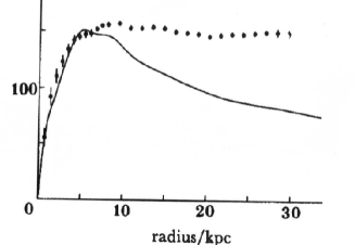
Figure 1: Observed Rotation velocity curve of the NGC3198 (error bars) and the prediction from Newtonian theory.

Except for the fact that dark matter interacts mainly through its gravitational field, not much is know about its other physical properties. This has motivated several attempts to dismiss dark matter altogether, regarding its gravitational effects as evidences for an alternative gravitational theory with respect to Newtonian theoryMilgrom ; Moffat , or for variants of general relativityBekenstein ; Freese ; Skordis . General relativity itself has been traditionally excluded from this analysis essentially because the slow motion of the observed objects usually leads to the Newtonian limit of the theory. This is reinforced by the fact that near the galaxies nuclei where the gravitational field is strong, like that of a black hole, the observed velocities closely agree with the prediction from Newton’s theory (as in Figure 1.), leading to the conclusion that Newton’s gravity should apply everywhere else, but a sufficient amount of dark matter must be added to increase the Newtonian gravitational pull. A recent review and check list for dark matter candidates can be found in Hooper ; Marco .

A qualitative distinction between dark matter gravity and baryons gravity was evidenced in the WMAP experiment Spergel . Referring to Figure 2, we quote : …”Cold dark matter serves as a significant forcing term that amplifies the higher acoustic oscillations. Alternative gravity models (e.g., MOND), and all baryons-only models, lack this forcing term so they predict a much lower third peak than is observed by WMAP and small scale CMB experiments”…

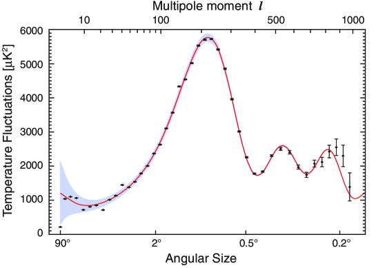
Figure 2: The observed power spectrum of the CBMR of the WMAP experience shows how the dark matter gravitational field can be different from the baryonic one.

These results were confirmed and sharpened by the observations of the luminous red galaxies in the Sloan Digital Sky Survey (SDSS), supporting the $\Lambda CDM$ model Tegmark . This was improved in the recent WMAP fifth year report WMAP5 .

As it seems evident, the study of dark matter gravity and its implications to the formation of structure in the early universe must naturally start with gravitational perturbation theory Rocky ; Mukhanov ; Padmanabham . The traditional gravitational perturbation mechanisms in relativistic cosmology are plagued by coordinate gauges, mostly inherited from the group of diffeomorphisms of general relativity. Fortunately there are some very successful criteria to filter out the latter perturbations Bardeen ; Geroch ; Walker , but they still depend on a choice of a perturbative model. A less known, but far more general approach to gravitational perturbation can be derived from a theorem due to John Nash, showing that any Riemannian geometry can be generated by a continuous sequence of local infinitesimal increments of a given geometry Nash ; Greene .

Nash’s theorem solves an old dilemma of Riemannian geometry, namely that the Riemann tensor is not sufficient to make a precise statement about the local shape of a geometrical object or a manifold. The simplest example is given by a 2-dimensional Riemannian manifold, where the Riemann tensor has only one component $R_{1212}$ which coincides with the Gaussian curvature. Thus, a flat Riemannian 2-manifold defined by $R_{1212}=0$ may be interpreted as a plane, a cylinder or a even a helicoid, in the sense of Euclidean geometry. Riemann regarded his concept of curvature as defining an equivalent class of manifolds instead of an specific one Riemann . While such equivalence of forms is mathematically interesting, it is less than adequate to derive physical conclusions from today’s sophisticated astronomical observations.

The solution to Riemann’s ambiguity problem was originally proposed in 1873 by L. Schlaefli Schlaefli , conjecturing that if a Riemannian manifold could be embedded in another one, then a decision on its real shape could be made by comparing the Riemann curvatures of the embedded surface with the one of the embedding space. The formal solution of this problem took a long time to be developed and it came only after the derivations of the conditions that guarantee the embedding of any Riemannian geometry into another, the well known Gauss-Codazzi-Ricci equations of geometry. The most general solution of the Schlaefli’s conjecture appeared only in 1956 with Nash’s theorem.

The Gauss-Codazzi-Ricci equations are non-linear and difficult to solve in the general case. Some simplifications were obtained by assuming that the metric is analytic in the sense that it is a convergence of a positive power series Cartan ; Janet . Nash’s theorem innovated the embedding problem by introducing the notion of differentiable, perturbative geometry: Using a continuous sequence of small perturbations of a simpler embedded geometry along the extra dimensions, he showed how to construct any other Riemannian manifoldGDE ; QBW . Nash’s approach to geometry not only solves the ambiguity problem of the Riemannian curvature, but also gives a prescription on how to construct geometrical structures by gradual deformations of simpler ones.

The purpose of this paper is to show that Nash’s geometric perturbative process contributes to explain the formation of structures in the universe. To see how this works, in the next section we show how the geometry of the standard cosmology regarded as submanifold embedded a 5-dimensional deSitter bulk, can be perturbed a la Nash, leading to a modified Friedman’s equation. We draw the theoretical CMBR power spectrum resulting from such perturbation, comparing it to the observed spectrum in the WMAP experiment. In section 3 we apply the same procedure for local dark matter gravity. However, since there are no evidences that the perturbative process is still going on today, except perhaps in young galaxies and cluster collisions where experimental data is still scarce, we assume as a first estimate that Nash’s perturbation is locally negligible in most spiral galaxies. This leads to a simpler set of equations where the brane-world gravitational equations reduce to the usual four-dimensional Einstein’s equations. In this case we will see that the motion of stars and of plasma substructures can be described by the application of ”slow geodesic motion” equation which holds true in an gravitational field of arbitrary strength and is not limited to the weak gravitational fields as in General Relativity.

II Dark Matter Cosmology

We start by reviewing some basic ideas of Nash’s geometric perturbation theorem: Suppose we have an arbitrarily given Riemannian manifold $\bar{V}_{n}$ with metric $\bar{g}_{\mu\nu}$, which is embedded into a given higher dimensional Riemannian manifold $V_{D}$, the bulk space. Then we may generate another metric geometry by a small perturbation $\bar{g}_{\mu\nu}+\delta g_{\mu\nu}$ where

$$\delta g_{\mu\nu}=-2\bar{k}_{\mu\nu a}\delta y^{a},\;\;a=N\!+\!1...D$$ (1)

where $\delta y^{a}$ denotes an infinitesimal variation of the extra dimensions orthogonal to $\bar{V}_{n}$ and $\bar{k}_{\mu\nu a}$ denote the extrinsic curvature components of $\bar{V}_{n}$ relative to the extra dimension $y^{a}$. Using this perturbation we obtain new extrinsic curvature $k_{\mu\nu a}$, and by repeating the process we obtain a continuous sequence of perturbations like

$$g_{\mu\nu}=\bar{g}_{\mu\nu}+\delta y^{a}\,\bar{k}_{\mu\nu a}+\delta y^{a}\delta y^{b}\,\bar{g}^{\rho\sigma}\bar{k}_{\mu\rho a}\bar{k}_{\nu\sigma b}\cdots$$

In this way any Riemannian geometry can be generated.

Nash’s original theorem used a flat D-dimensional Euclidean space but this was soon generalized to any Riemannian manifold, including those with non-positive signatures Greene . Although the theorem could also be generalized to include perturbations on arbitrary directions in the bulk, it would make its interpretations more difficult, so that we retain Nash’s choice of independent orthogonal perturbations. It should be noted that the smoothness of the embedding is a primary concern of Nash’s theorem. In this respect, the natural choice for the bulk is that its metric satisfy the Einstein-Hilbert principle. Indeed, that principle represents a statement on the smoothness of the embedding space (the variation of the Ricci scalar is the minimum possible). Admitting that the perturbations are smooth (differentiable), then the embedded geometry will be also differentiable.

The Einstein-Hilbert principle leads to the D-dimensional Einstein’s equations for the bulk metric ${\cal G}_{AB}$ in arbitrary coordinates

$${\mathcal{R}}_{AB}-\frac{1}{2}\mathcal{R}\mathcal{G}_{AB}=\alpha_{*}T^{*}_{AB}$$ (2)

where we have dispensed with bulk cosmological constant and where $T^{*}_{AB}$ denotes the energy-momentum tensor of the known matter and gauge fields. The constant $\alpha_{*}$ determines the D-dimensional energy scale.

The four-dimensionality of the space-time manifold is an experimentally established fact, associated with the Poincar invariance of Maxwell’s equations and their dualities, later extended to all gauge fields. Therefore, all matter which interacts with these gauge fields must for consistency be also defined in the four-dimensional space-times. On the other hand, in spite of all efforts made so far, the gravitational interaction has failed to fit into a similar gauge scheme, so that the gravitational field does not necessarily have the same four-dimensional limitations and it can access the extra dimensions in accordance with (1), regardless the location of its sources.

We assume that the four-dimensionality of gauge fields and ordinary matter applies to all perturbed space-times, so that it corresponds to a confinement condition. In order to recover Einstein’s gravity by reversing the embedding, the confinement of ordinary matter and gauge fields implies that the tangent components of $\alpha_{*}T^{*}_{AB}$ in the above equations must coincide with $8\pi GT_{\mu\nu}$ where $T_{\mu\nu}$ is the energy-momentum tensor of the confined sources .

Since dark matter gravity is not necessarily confined, it also propagates in the bulk. Furthermore, based on the lack of experimental evidences on the energy-momentum of the dark matter in the bulk, we also assume that the normal and the cross components of the dark matter energy-momentum tensor, respectively $T_{\mu a}$ and $T_{ab}$ vanish, meaning that there are no known sources outside the four-dimensional space-times.

The standard Friedman-Lemaitre-Robertson-Walker (FLRW) universe can be embedded without restrictions in a five-dimensional. Therefore, using the Einstein equation (2) written in the Gaussian frame defined by the four-dimensional submanifold, we obtain the equations of the FLRW embedded geometryGDE

$$R_{\mu\nu}-\frac{1}{2}Rg_{\mu\nu}-{Q}_{\mu\nu}=-8\pi GT_{\mu\nu}$$ (3)

$$k_{\mu;\rho}^{\rho}\!-\!h_{,\mu}=0$$ (4)

where now $T_{\mu\nu}$ is the energy-momentum tensor of the confined perfect fluid, $k_{\mu\nu 5}\equiv k_{\mu\nu}$ denotes the components of the extrinsic curvature of the embedded space-time, $h=g^{\mu\nu}k_{\nu\nu}$, $K^{2}=k^{\mu\nu}k_{\mu\nu}$ and

$$Q_{\mu\nu}=k^{\rho}{}_{\mu}k_{\rho\nu}-hk_{\mu\nu}\!\!-\!\!\frac{1}{2}(K^{2}-h^{2})g_{\mu\nu}.$$ (5)

This tensor is independently conserved, as it can be directly verified that (semicolon denoting covariant derivative with respect to $g_{\mu\nu}$)

$$Q^{\mu\nu}{}_{;\nu}=0$$ (6)

In coordinates $(r,\theta,\phi,t)$ the FLRW model can be expressed s Rosen :

$$ds^{2}=-dt^{2}+a^{2}(t)[dr^{2}+f_{k}^{2}(r)(d\theta^{2}+\mbox{sin}^{2}\theta d\phi^{2})]$$ (7)

where $f_{k}(r)=r,\mbox{sin}\,r,\mbox{sinh}\,r$ corresponding to $k=0,+1,-1$ (spatially flat, closed, open respectively). We start solving (4) for the above metric in the deSitter bulk. It is easier to find the solution of Codazzi’s equations

$$k_{\mu[\nu;\rho]}=0$$

of which (4) is just its trace. The general solution of this equation is

$$k_{ij}=\frac{b}{a^{2}}g_{ij},\;\;\,k_{44}=-\frac{1}{\dot{a}}\frac{d}{dt}\left(\frac{b}{a}\right)\;\;i,j=1\ldots 3$$ (8)

Defining $B=\frac{\dot{b}}{b}$, we may express the components of $Q_{\mu\nu}$ as

$$Q_{ij}=\frac{b^{2}}{a^{4}}\left(2\frac{B}{H}-1\right)g_{ij},\;\;\;Q_{44}=-\frac{3b^{2}}{a^{4}},\;\;\;Q=-\frac{6b^{2}}{a^{4}}\frac{B}{H},\;\;\;i,j=1..3$$ (9)

where $H=\dot{a}/a$ is the usual Hubble parameter. After replacing in (3) we obtain Friedman’s equation modified by the extrinsic curvature:

$$(\frac{\dot{a}}{a})^{2}+\frac{k}{a^{2}}=\frac{8\pi G}{3}\rho+\frac{b^{2}}{a^{4}}$$ (10)

To interpret this result we have compared it with the XCDM, phenomenological x-fluid model, with state equation $p_{x}=\omega_{x}\rho_{x}$, which corresponds to the geometric equation on $b(t)$

$$\frac{\dot{b}}{b}=\frac{1}{2}(1-3\omega_{x})\frac{\dot{a}}{a}$$ (11)

This cannot be readily integrated because $\omega_{x}$ is not known. However, in the particular case when $\omega_{x}=\omega_{0}$=constant, we obtain a simple solution

$$b(t)=b_{0}(\frac{a}{a_{0}})^{\frac{1}{2}(1-3\omega_{0})}$$ (12)

where $a_{0}$ and $b_{0}\neq 0$ are integration constants. Replacing this solution in (10) we obtain an accelerated universe which is consistent with the most recent observations, when the values of $\omega_{0}$ are taken within the range $-1\leq\omega_{0}\leq-1/3$ GDE . Furthermore, the theoretical power spectrum obtained from the extrinsic curvature perturbation of the FLRW model, is not very different from the observed power spectrum in the WMAP/5y, displayed in Fig. 2.

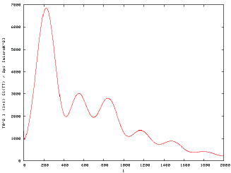
Figure 3: The theoretical power spectrum calculated with the CAMB for $-1\leq\omega_{0}\leq-1/3$, Massive Neutrinos=1, massless neutrinos =3.04.

III Local Dark Matter Gravity

It is possible that in young galaxies which are still in the process of formation Puzia ; in galaxies with active galaxy nuclei deVries ; or even in cluster collisions, Nash’s perturbations could be applied, where the metric symmetry is taken to be local. However, there not sufficient experimental data to support such local perturbations. Therefore, in the following we restrict our study on local dark matter gravity to the cases where Nash’s perturbations has ceased. From (1) we see that this limiting condition is given by $k_{\mu\nu}$. Furthermore, if $T_{\mu\nu}$ is composed by ordinary matter and gauge fields, the rsulting equations are the same as the vacuum Einstein’s equations

$$R_{\mu\nu}-\frac{1}{2}Rg_{\mu\nu}=0$$ (13)

These equations are be understood in the context of the embedded space-times and with the confinement conditions for ordinary matter and gauge fields. They do not represent the whole of General Relativity because the principle of general covariance does not necessarily apply to the bulk geometry. This follows from the fact that Nash’s perturbations are restricted to be along the orthogonal directions only.

The recently observed correlation between the highest-energy cosmic rays sources and active galactic nucleiAuger suggests the existence of strong gravitational fields in those regionsRichstone ; Ferrarese1 ; Ferrarese2 . Nonetheless, the observed motion of stars near black holes observed at the nuclei of some of these galaxies indicate that the velocities are small, of the order of a few hundreds of kilometers per second. This requires the description of a slow geodesic motion in the presence of strong gravitational fields In what follows we use essentially the first part of the exposition in the Misner, Thorn & Wheeler’s book Wheeler .

Consider a slow free falling particle (or star) in a gravitational field described by a solution of the vacuum Einstein’s equations (like in (13) in a suitable coordinate system. Initially the particle is located in a far away region, where the action of the gravitational field is supposedly weak, and we can write (The notation $h_{\mu\nu}$ reminds that this is not Nash’s perturbation)

$$g_{\mu\nu}=\eta_{\mu\nu}+\delta h_{\mu\nu},\;\;\mbox{where}\;\;\delta h^{2}_{\mu\nu}<<\delta h_{\mu\nu},$$ (14)

Here the small deviation from Minkowski’s metric has nothing to do with the velocity of the particle. However, since $v<<1$, we can use Newtonian coordinates (with $x^{4}=t$, $t$ being the Newtonian time), so that the spatial components of the geodesic equations become

$$\frac{d^{2}x^{i}}{dt^{2}}=-\Gamma^{i}_{\mu\nu}\frac{dx^{\mu}}{dt}\frac{dx^{\nu}}{dt}-2\Gamma^{i}_{\mu 4}\frac{dx^{\mu}}{dt}=-\Gamma_{44}^{i}=-\frac{1}{2}\delta h_{44,i},\;\;\;i,j=1..3$$ (15)

At this point a scalar field $\varphi$ may be defined such that

$$\frac{d^{2}x^{i}}{dt^{2}}=-\frac{\partial\varphi}{\partial x^{i}}$$ (16)

Comparing (15) and (16) we obtain an equation to determine the field $\varphi$:

$$\frac{\partial\varphi}{\partial x^{i}}=-\frac{1}{2}\delta_{ij}\frac{\partial\delta h_{44}}{\partial x_{j}}$$ (17)

As the particle continues its fall, the gravitational pull continuously builds up by small increments of the metric as in

$$g_{\mu\nu}\approx\eta_{\mu\nu}+\delta h_{\mu\nu}+(\delta h_{\mu\nu})^{2}+\cdots$$

Actually, there is no way to stop this process without applying an external force. Thus, equation (17) can be integrated along the geodesic, where $\delta h_{\mu\nu}$ continuously increase up to a finite value $h_{\mu\nu}$, leading to the scalar gravitational potential (often referred to as the nearly Newtonian potential, not to be confused with the post Newtonian approximations):

$$\varphi=-\frac{1}{2}\int_{0}^{h_{44}}d(\delta h_{44})=-\frac{1}{2}(1+g_{44})$$ (18)

Notice that except at the beginning of the free fall a weak gravitational field was not imposed. Here $g_{44}$ is obtained from an exact solution of Einstein’s equations, so that at the end all metric components $g_{\mu\nu}$ contribute to (18). In the following we exemplify this application of (18) to the motion of stars in galaxies and clusters.

%subsubsectionRotation Velocity curves in Galaxies

The gravitational field of a simple disk galaxy model can be obtained from the cylindrically symmetric Weyl metric, expressed in cylindrical coordinates $(r,z,\theta,t)$ as Weyl :

$$dS^{2}=e^{2(\lambda-\sigma)}dr^{2}+r^{2}e^{-2\sigma}d\varphi^{2}+e^{2(\lambda-\sigma)}dz^{2}-e^{2\sigma}dt^{2}$$ (19)

where $\lambda=\lambda{(r,z)}$ and $\sigma=\sigma{(r,z)}$. As shown in Rosen ; Zipoy , the Weyl cylindrically symmetric solution is diffeomorphic to the Schwarzschild solution. Replacing the Weyl metric with these conditions in (3) and (6) we obtain

$$-\lambda_{,r}+r\sigma_{,r}^{2}-r\sigma_{,z}^{2}=0$$ (20)

$$-\sigma_{,r}-r\sigma_{,rr}-r\sigma_{,zz}=0$$ (21)

$$\lambda_{,rr}+\lambda_{,zz}+\sigma_{,r}^{2}+\sigma_{,z}^{2}=0$$ (22)

$$2r\sigma_{,r}\sigma_{,z}=\lambda_{,z}$$ (23)

The cylinder solution is diffeomorphic to a Schwarzschild’s solution.

In the following we apply this solution to find a the geodesic motion of slowly free falling star under the gravitational field in the galactic plane. Since the slow motion geodesic equation (16) is not invariant under diffeomorphisms, we may consider three separate stages separately, in accordance with the symmetry of the gravitational field which is effective at the current position of the star:

(A) The star is far away from the galaxy:
In this case, the gravitational field of the galaxy is weak, like that of a point source. Therefore, the predominant gravitational field is given by the exterior Schwarzschild solution, as seen from a large distance from the galaxy nucleus. In spherical coordinates, we can write the metric component $g_{44}=-(1-2M/r)$, and (18) gives

$$\varphi\rfloor_{Newton}=-M/r,\;\;\;r>>r_{0}$$

which is equivalent to the Newtonian gravitational potential produced by a distant mass $M$, determined by the Newtonian (weak field) limit. In such situation (18) agrees with all estimates resulting from the Newtonian gravitational theory for a spherically symmetric dark matter halo, producing the same rotation velocity curves.
(B) The star is close to the galaxy’s disk:
When the star is close to the galaxy, in the disk plane, the predominant dark matter gravitational field can be simulated by the vacuum cylindrically symmetric Weyl metric, satisfying the vacuum Einstein’s equations (20) to (23). However, to configure a disk galaxy we need to apply the condition that Weyl’s cylinder has a thickness that is much smaller than its radius: $h<<r_{0}$. With this condition we can no longer apply the diffeomorphism invariance of general relativity, so that the solution must be written in cylindrical coordinates.

The disk-symmetry condition can be written as $z\in[-h_{0}/2,h_{0}/2],\;\;\;\mbox{for}\;\;\;r\in[0,r_{0}],\;\;\;h_{0}<<r_{0}$, so that the functions $\sigma(r,z)$ and $\lambda(r,z)$ may be expanded around $z=0$ as

$$\phantom{x}\sigma(r,z)=\sigma(r,0)+za(r)+\cdots$$

$$\phantom{x}\lambda(r,z)=\lambda(r,0)+zb(r)+\cdots$$

where we have denoted $a(r)=\left.\frac{\partial\sigma(r,z)}{\partial z}\right\rfloor_{z=0}\;\;\mbox{and}\;\;\,b(r)=\left.\frac{\partial\lambda(r,z)}{\partial z}\right\rfloor_{z=0}$. Neglecting the higher order terms, it follows that equations (21) and (23) become a simple system of equations on $\sigma$, with general solution $\sigma(r,z)=\frac{K}{2}\ln r+c_{2}(z)$ where $c_{2}(z)$ is an r-integration constant and where we have denoted $K={b(r)}/{a(r)}$. Derivation of $\sigma$ with respect to $z$ gives $c_{2}(z)=a(r)z+c_{0}$, but since $c_{2}$ does not depend on $r$, it follows that $a(r)$ must be a constant $a_{0}$. By similar arguments we find that $b(r)=b_{0}=$constant, so that $K=K_{0}=b_{0}/a_{0}$ is also a constant. Replacing these results in (20) and (22), we again obtain another simple solvable system of equations in $\lambda$, so that the solution of the vacuum Einstein’s equations for the Weyl disk is

$$\sigma(r,z)=\frac{K_{0}}{2}\ln r+a_{0}z+c_{0}$$ (24)

$$\lambda(r,z)=\frac{K_{0}^{2}}{2}\ln r-a_{0}\frac{r^{2}}{2}+b_{0}z+d_{0}$$ (25)

where $c_{0}$ and $d_{0}$ are again integration constants. From (24) we obtain $g_{44}=-e^{2\sigma}=-e^{2\frac{K_{0}}{2}\ln r}e^{2a_{0}z}e^{2c_{0}}$. Therefore, for a star near the galaxy in the galaxy plane $z=0$, in the region between the nucleus radius $r_{c}$ and the disk radius $r_{0}$ (18) is

$$\varphi\rfloor_{disk}=-\frac{1}{2}(1+g_{44})\rfloor_{z=0}=-\frac{1}{2}(1-e^{2c_{0}}r^{K_{0}}),\;\;\;r_{c}<r<r_{0}$$ (26)

Here we cannot make use of the Newtonian limit to determine the integration constant $e^{2c_{0}}$ in (26), because we do not have the same symmetry and the same boundary conditions appropriate for the Newtonian gravitational field. Instead, we may compare (26)with the local Newtonian potential produced by a disk of visible mass M, suggesting that the above integration constant can be written as proportional to the to the total baryonic mass $M_{b}$ of the galaxy. Thus, in units G=c=1 we set $e^{2c_{0}}K_{0}/2=\beta_{0}M_{b}$, where $\beta_{0}$ is a mass scale factor, proportional to the estimated visible mass of the galaxy Salucci .

The rotation velocity of a test particle under (18) is $v=\omega_{0}r$, $\omega_{0}=$ constant, obtained by comparing the radial force $\frac{v^{2}}{r}\hat{r}$, with $-\frac{\partial\varphi}{\partial r}\hat{r}$, so that the velocity is given by $v=\sqrt{|r\frac{\partial\varphi}{\partial r}|}$. In the particular case of the disk, using (26) we obtain

$$v(r)=\sqrt{|\beta_{0}M_{b}r^{K_{0}}|},\;\;\;r_{c}<r<r_{0}$$ (27)

Here $K_{0}$ represents the ratio between the coefficients $a(r)$ and $b(r)$ of the expansion of the metric functions $\sigma$ and $\lambda$ respectively. In the considered linear expansion in (24) and (25), $K_{0}$ can be adjusted experimentally. In practice it can be scaled by a constant, so as to belong to interval between $0$ and $1$, corresponding to the galaxy nucleus radius where the spherical symmetry applies, and to the distance where the disk symmetry applies. The extreme values in that interval are excluded: The value $K_{0}=0$ is excluded because for that value the potential (26) does not exert any force. The value $K_{0}=1$ is also excluded because it gives velocity proportional to $\sqrt{r}$ which is not experimentally verified.

Using the minimum square root curve fitting, figures 2, 3 and 4 show the velocities near the disk, calculated with (27) for some known galaxies (red dots) for $r$ larger than the estimated core radius where the disk symmetry applies. The values of the two free parameters $K_{0}$ and $\beta_{0}$ in each case were determined by the minimum squares numerical iteration method, extracted from known experimental data Sanders . For comparison purposes, we included the black error bars showing the measured velocities and the green triangles corresponding to the Newtonian predictions.

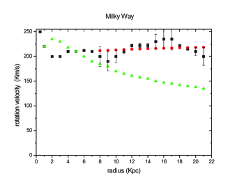
Figure 4: Via Lactea with $M_{b}=1.99\times 10^{41}$Kg, $R=8,5$Kpc, $K_{0}=0.0682$ and $\beta_{0}=0.0901$.

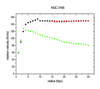
Figure 5: NGC3198, with $M_{b}=1.19\times 10^{40}$Kg, $R=16,6$Kpc, $K_{0}=0.0162$ and $\beta_{0}=0.8224$

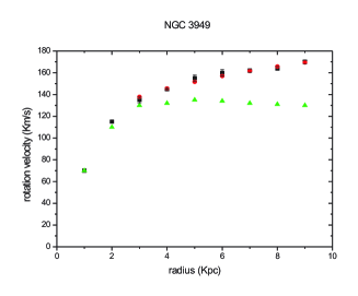
Figure 6: NGC3949, with $M_{b}=4.97\times 10^{39}$Kg, $R=6$Kpc, $K_{0}=0.3766$ and $\beta_{0}=1.1657$

(C) The star is near the galaxy’s nucleus:
When the star reach the nucleus of the galaxy, the observed velocity is still small, but the gravitational field is likely to be strong. A simple configuration of the gravitational field acting on the star can be obtained if we neglect the rotation of the galaxy’s nucleus, so that we obtain a spherically symmetric gravitational field, described by the by the Schwarzschild solution of (13) with $g_{44}=-(1-2M/r)$. Then we obtain from (18)

$$\phi\rfloor_{Nucleus}=-M/r,\;\;\;r\leq r_{c}$$ (28)

and the star rotation velocity is given by $v(r)=\sqrt{{M}/{r}}$, were now $M$ is associated with the Schwarzschild mass of the Nucleus. Thus, the velocity looks exactly like the one in the Newtonian theory, with the exception that the gravitational field is not necessarily weak. This is a consequence of the assumed metric symmetry at the galaxy’s nucleus.

Two recent observations of colliding cluster dark matter halos have provided new insights on the dark matter gravity issue: One of them is the bullet cluster 1E0657-558, showing the motion of a sonic boom effect in the intercluster plasma with velocity $\sim 4700$km/s, visible through x-ray astronomy Clowe . Under the assumption that the gravitational field of the two clusters is Newtonian and the existence of gravitational field of dark matter halos in each cluster, the (linear) superposition of the two dark matter gravitational fields produce a center of mass of the system which coincides with the observed position of the plasma bullet. This has been claimed to be an observational evidence for the existence of dark matter.

On the other hand, using (18) instead of the Newtonian gravity, and admitting that the gravitational field of each cluster is spherically symmetric, we have the gravitational field of the spherically symmetric dark matter halos would be given by two separate Schwarzschild solutions. Then the action of each of these gravitational field on the plasma can be taken as in (28), which resembles the Newtonian potential, producing the same center of mass as described in Newtonian theory. However, such superposition of two Schwarzschild’s solution is only a crude approximation to compare with the dark matter halos. To be more precise, either we consider a two body problem solution of (13), or else we consider the cluster collision as a Nash’s perturbation process. In the latter case we may start with an embedded spherically symmetric cluster which is perturbed by the extrinsic curvature generated by the second cluster according to (1). This is easier said than done, because the differentiable embedding of a Schwarzschild solution requires six dimensions. Nonetheless, in principle this solution can be calculated and tested.

The second observation is that of the Abel 520 cluster MS0451+02, showing again two colliding ”dark matter halos”, where at least one of them do not seem to be anchored to a baryonic structure. The most immediate explanation is that this ”pure dark matter halos” may be an evidence of a non-linear effect of the dark matter gravitational field, which does not agree with the Newtonian gravitational field assumption. So, in a sense this observation backs up the hypothesis of a non-linear alternative gravitational theory at the galaxy/cluster scale of observations.

In particular it is possible to explain the existence of a gravitational effect which is not anchored to a baryonic source as a solution of (13), as a for example a vacuum Schwarzschild solution or a Weyl disk solution, which may act as a perturbation to another cluster, again applying (1) to find the final gravitational field of the system. The result may be compared with the motion of the x-ray observed plasma structure. However, we are still pending on further details on the Abel 520 collision.

IV Summary

Gravitational perturbation theory has become an essential tool for the explanation of the formation of large structures in the universe. Here we have presented an application of Nash’s theorem on perturbations of geometries to the formation of space-time structures and to explain the local effects usually attributed to dark matter. In a brief justification we have argued that the theorem improves Riemann’s geometry in the sense that it replaces the somewhat absolute notion of Riemann curvature, by a relative notion of curvature with respect to the Riemann tensor of the bulk defined by the Einstein-Hilbert principle.

The relevant detail in Nash’s theorem, is that it provides a mathematically sound and coordinate gauge free way to construct any Riemannian geometry, and in particular any space-time structures, by a continuous sequence of infinitesimal perturbations along the extra dimensions of the bulk space, generated by the extrinsic curvature.

The four-dimensionality of space-time is regarded here as an experimental fact, related to the symmetry properties of Maxwell’s equations or, more generally of the gauge theories of the standard model. Thus, any matter that interacts with gauge fields, including the observers, must remain confined to four-dimensions. However, in accordance with Nash’s theorem, gravity as represented by a metric cannot be confined because it is perturbable along the extra dimensions.

In a first cosmological application of that theorem we have compared our results with the present observational data. Starting with the FLRW cosmological model embedded in the five-dimensional deSitter bulk, and applying equations (3) and (4). We have found that Friedman’s equation is necessarily modified by the presence of the extrinsic curvature. We have shown that this modification is consistent with the observed acceleration of the universe, including with the observed power spectrum of the CMBR.

In principle the local effects of dark matter gravitation should have the same explanation, although they have different observational aspects. The simplest case is that of the rotation curves in galaxies and galaxy clusters, which originated the dark matter issue. In this case, there is no evidence that the gravitational perturbation process is still active, except perhaps in young galaxies. Therefore, we have considered the case where Nash’s perturbations vanish, obtaining the vacuum Einstein’s equations, applied to the metric with an specific symmetry. Instead of the Newtonian potential we have applied the geodesic equations for slow motion. Using the Weyl metric to simulate a disk galaxy, we have compared the result with some known cases.

More recently the observations of merging clusters have provided additional information on the dark matter issue. The slow motion of the plasma substructures can be handled by the same equations but it appears to us that the correct formulation of the problem should be made with Nash’s perturbative analysis.

References

- (1) F. Zwicky, Helv. Phys. Acta, 6, 110 (1933)
- (2) R. B. Tully & J.R. Fisher, Astron. & Astrophys. 54, 661 (1977)
- (3) T. S. Van Albada, and R. Sancisi, Phil. Trans. R. Soc. London, A 320, 447 (1986)
- (4) Y. Sufue, The Astrophysical Journal 458, 120, (1996), astro-ph/0010595
- (5) M. Milgrom, The Astrophysical Journal 270, pag. 365, Ibid pag. 371, Ibid, pag. 384 (1983)
- (6) J.R. Brownstein & J.W. Moffat, Astrophysisical Journal 636, (2006), astro-ph/0506370
- (7) J. Bekenstein and M. Milgrom, The Astrophysical Journal 286, 7, (1984)
- (8) K. Freese, New Astron.Rev. 49, 103, (2005), astro-ph/0501675
- (9) C. Skordis, D. F. Mota, P.G. Ferreira, & D. Boehm, Phys. rev. Lett. 96, 011301 (2006)
- (10) S. Dodelson, Phys. Rev. Lett. 97, 231301, (2006), astro-ph/0608602
- (11) Dan Hopper & E. A. Blatz, arXiv:0802.0702V2
- (12) Marcos Taoso, Gianfranco bertone & Antonio Masiero, arXiv:0711.4996v2
- (13) D.N. Spergel et al, Astrophys.J.Suppl. 170, 377 (2007), astro-ph/0603449
- (14) Max Tegmark et al. Phys.Rev. D74, 123507 (2006), astro-ph/0608632. See also the SDSS phase 3 at http://sdss3.org
- (15) E. Komatsu et al, (WMAP/5y, arXiv:0803.0547
- (16) E. Kolb & M.S. Turner, The Early Universe, Addison-Wesley (1990)
- (17) V. F. Mukhanov, H. A. Feldman & R. H. Brandenberger, Phys. Rep. 5, 6, 203-333, (1992)
- (18) T. Padmanabham, Structure Formation in the Universe, Cambridge U. press, (1993)
- (19) J. Bardeen, Phys. Rev. D31, 1792 (1985)
- (20) R. Geroch, Comunn. Math. Phys. 13, 180 (1969)
- (21) J. M. Stewart and M. Walker, Proc. Roy. Soc. (London), A341, 49 (1974)
- (22) J. Nash, Ann. Maths. 63, 20 (1956)
- (23) R. Greene, Memoirs Amer. Math. Soc. 97, (1970)
- (24) B. Riemann (Translated by W. K. Clifford), Nature 8, 114 and 136 (1873)
- (25) L. Schlaefli, Ann. di mat. ( series), 5, 170-193 (1871)
- (26) E. Cartan, Ann. Soc. Pol. Mat 6, 1, (1927)
- (27) M. Janet, Ann. Soc. Pol. Mat 5, (1928)
- (28) J. E. Campbell, A Course of Differential Geometry, Claredon Press, Oxford (1926)
- (29) F. Dahia, C. Romero, Braz.J.Phys. 35, 1140, (2005)
- (30) M.D. Maia , E.M. Monte, J.M.F. Maia, J.S. Alcaniz. C.Q.G. 22 1623 (2005), astro-ph/0403072
- (31) M.D. Maia, Nildsen Silva, M.C.B. Fernandes, JHEP 04, 047 (2007), arXiv:0704.1289 [gr-qc]
- (32) T. H. Puzzia, B. Mobasher & P. Goudfrooij, arXiv:0705.4092
- (33) N. de Vries, et al, arXiv:0708.2672
- (34) The Pierre Auger Collaboration, Science, 318, 938, (2007), DOI: 101126/Science.1151124
- (35) D. Richstone et al, Nature 395, A14, (1998)
- (36) L. Ferrarese & H. Ford astro-ph/0411247
- (37) L. Ferrarese & D. Merrit, Phys.World 15N6, 41-46, (2002), astro-ph/0206222
- (38) C. Misner, K.S. Thorne & J. A. Wheeler, Gravitation, W.H. Freeeman & co. 1st ed. p. 412 ff.
- (39) H. Weyl, Ann. Phys. 54, 117 (1917)
- (40) N. Rosen, Rev. Mod. Phys. 21, 503, (1949
- (41) D. M. Zipoy, Jour. Math. Phys. 7, 1137 (1966)
- (42) M.A.H. MacCallum, 28th Spanish Relativity Meeting (ERE05). AIP Conf.Proc.841:129-143,2006, gr-qc/0601102. Also, H. Stephani et al, Exact Solutions of Einstein’s Field Equations, ed, Cambridge Monographs on Mathematical Physics, C.U. Press (2003)
- (43) M. Persic et al, Mon. Not. R. Astron. Soc. 281, 27, (1996); P. Salucci & M.Persic, astro-ph/9601018; F. Shankar et al, astro-ph/0601577
- (44) Legacy Archive for Microwave Background Data Analysis, http://lambda.gsfc.nasa.gov
- (45) R. H. Sanders & M. A. W. Verheijen, ApJ 503, 97 (1998). R. H. Sanders, ApJ 473, 117 (1996)
- (46) D. Clowe et al, Astrophys.J.648, L109-L113,(2006), astro-ph/0608407
- (47) A Dark Core in Abell 520. A. Mahdavi, H.y Hoekstra, A.y Babul, D.y Balam, P. Capak arXiv:0706.3048
- (48) L.P. Eisenhart, Princeton U. P. Sixth print, p.159 ff, (1966).