The local content of bipartite qubit correlations

Abstract

One of the last open problems concerning two qubits in a pure state is to find the exact local content of their correlation, in the sense of Elitzur, Popescu and Rohrlich (EPR2) [Phys. Lett. A 162, 25 (1992)]. We propose a new EPR2 decomposition that allows us to prove, for a wide range of states $\mbox{$|\psi(\theta)\rangle$}=\cos\theta\mbox{$|00\rangle$}+\sin\theta\mbox{$|11\rangle$}$, that their local content is $\bar{p_{L}}(\theta)=\cos 2\theta$. We also share reflections on how to possibly extend our result to all two-qubit pure states.

I Introduction

The incompatibility of quantum mechanics with local variable theories, as shown by Bell Bell (1964), lies at the statistical level: local variable theories cannot reproduce all statistical predictions of quantum theory. In a typical Bell experiment, one observes correlations between the measurement results of two partners (Alice and Bob), and averages them over measurements on many pairs of particles. One may then conclude that non-locality was observed if the average correlations thus obtained violate a Bell inequality.

However, if the statistics of the observations exhibit non-locality, it does not imply that all individual pairs behave non-locally. This observation lead Elitzur, Popescu and Rohrlich Elitzur et al. (1992), hereafter referred to as EPR2, to wonder whether one could consider that a fraction of the pairs still behaves locally, while another fraction would behave non-locally (and possibly more non-locally than quantum mechanics allows).

More explicitly, writing $P_{Q}$ the quantum mechanical probability distribution for Alice and Bob’s results, the EPR2 approach consists in decomposing $P_{Q}$ as a convex sum of a local part, $P_{L}$, and of a non-local part, $P_{NL}$, in the form

$$P_{Q}=p_{L}P_{L}+(1-p_{L})P_{NL},\quad\textrm{with }p_{L}\in[0,1].$$ (1)

The maximal weight $\bar{p_{L}}=\max p_{L}$ that can be attributed to the local part can be regarded as a measure of (non-)locality of the quantum distribution $P_{Q}$. Finding this maximal possible local weight is not a trivial problem; so far one only knows how to calculate lower and upper bounds on $\bar{p_{L}}$.

In this paper, we concentrate on the simplest case of a quantum probability distribution originating from Von Neumann measurements on two-qubit pure states. After recalling previously known results for this case, we propose a new EPR2 decomposition and derive a new lower bound on $\bar{p_{L}}$, which reaches the previously known upper bound Scarani (2008) for a wide class of states. This gives a definite value for the exact local content $\bar{p_{L}}$ of those states. We then share reflections on how one might possibly extend our result to all two-qubit pure states.

II The EPR2 approach for two-qubit pure states

II.1 Correlations of two-qubit pure states

Without loss of generality, any two-qubit pure state can be written in the form

$$\mbox{$|\psi(\theta)\rangle$}=\cos\theta\mbox{$|00\rangle$}+\sin\theta\mbox{$|11\rangle$}$$ (2)

with $\theta\in[0,\frac{\pi}{4}]$. In the following, we shall use the notation $c=\cos 2\theta,s=\sin 2\theta$ (with $c,s\in[0,1]$).

Each qubit is subjected to a Von Neumann measurement, labeled by unit vectors $\vec{a}$ and $\vec{b}$ on the Bloch sphere $S^{2}$. Let us denote by $a_{z}$ and $b_{z}$ the $z$ components of $\vec{a}$ and $\vec{b}$, by $a_{\perp}=\sqrt{1-a_{z}^{2}}$ and $b_{\perp}=\sqrt{1-b_{z}^{2}}$ the amplitudes of the components of $\vec{a}$ and $\vec{b}$ in the $xy$ plane, and by $\chi\in\,]\!-\pi,\pi]$ the difference between the azimuthal angles of $\vec{a}$ and $\vec{b}^{\prime}$, with $\vec{b}^{\prime}$ defined as the reflection of $\vec{b}$ with respect to the $xz$ plane.

With these notations, and for binary results $\alpha,\beta=\pm 1$, quantum mechanics predicts the following conditional probability distribution:

$$\begin{array}[]{rcl}P_{Q}(\alpha,\beta|\,\vec{a},\vec{b})&=&\frac{1}{4}\big{(}1+\alpha\,M_{Q}(\vec{a})+\beta\,M_{Q}(\vec{b})\\ &&\qquad\quad+\ \alpha\beta\,E_{Q}(\vec{a},\vec{b})\big{)}\end{array}$$ (5)

$$\mathrm{with}\quad M_{Q}(\vec{a})=c\,a_{z},\quad M_{Q}(\vec{b})=c\,b_{z},$$ (6)

$$\begin{array}[]{rl}&E_{Q}(\vec{a},\vec{b})=a_{z}b_{z}+s\,(a_{x}b_{x}-a_{y}b_{y})\\ &\phantom{E_{Q}(\vec{a},\vec{b})}=a_{z}b_{z}+s\,a_{\perp}b_{\perp}\cos\chi\,.\end{array}$$ (9)

As explained before, the EPR2 problem is to find a decomposition of $P_{Q}(\alpha,\beta|\,\vec{a},\vec{b})$ as a convex sum of a local and a non-local probability distribution, in the form (1). For a given state (i.e., a given value of $\theta$), the equality is required to hold for all possible measurements $\vec{a},\vec{b}$ and for all results $\alpha,\beta$. The weight $p_{L}\in[0,1]$ of the local distribution should be independent of the measurements and of the outcomes.

The probability distribution $P_{L}(\alpha,\beta|\,\vec{a},\vec{b})$ is required to be local, in the sense that it can be explained by local variables $\lambda$, i.e. it can be decomposed in the form

$$P_{L}(\alpha,\beta|\,\vec{a},\vec{b})=\int\mathrm{d}\!\lambda\,\rho(\lambda)\ P^{A}_{\lambda}(\alpha|\vec{a})P^{B}_{\lambda}(\beta|\vec{b}).$$ (10)

On the other hand, no restriction is imposed on $P_{NL}$, except that it must be non-negative for all inputs and outputs:

$$P_{NL}=\frac{1}{1-p_{L}}(P_{Q}-p_{L}P_{L})\,\geq\,0\ .$$ (11)

In particular, $P_{NL}$ is allowed to be even more non-local than quantum mechanical correlations.

The goal is to find, for a given state, a decomposition with the largest possible value for $p_{L}$, denoted $\bar{p_{L}}(\theta)$, which characterizes the locality of the probability distribution $P_{Q}$ as defined by (5–9).

II.2 Previously known results and conjecture

In their original paper Elitzur et al. (1992), Elitzur, Popescu and Rohrlich proposed an explicit local probability distribution $P_{L}$, which lead to an EPR2 decomposition with $p_{L}=\frac{1-s}{4}$. This was the first known lower bound on $\bar{p_{L}}(\theta)$. Clearly, this was not optimal, at least when approaching the product state ($\theta=0$, i.e., $s=0$) which is fully local, and therefore satisfies $\bar{p_{L}}(0)=1$.

They also argued that for the maximally entangled state ($\theta=\pi/4$), $P_{Q}$ contains no local part: $\bar{p_{L}}(\frac{\pi}{4})=0$, i.e. no EPR2 decomposition with $p_{L}>0$ exists for this state. This is in fact a much more general result, as shown later by Barrett et al Barrett et al. (2006): the maximally entangled state of two $d$-dimensional quantum systems, for any dimension $d$, has no local component.

In Scarani (2008), one of the authors could improve on the first lower bound for $\bar{p_{L}}(\theta)$, as he gave an explicit decomposition that achieves $p_{L}=1-s$. Interestingly, it was noted that this is the largest possible value that can be attributed to $p_{L}$, if $P_{L}$ depends only on the $z$ components $a_{z}$ and $b_{z}$ of $\vec{a}$ and $\vec{b}$. Recently, this bound ($\bar{p_{L}}\geq 1-s$) has been extended to mixed two-qubit states by noticing that $s$ is actually the concurrence of the state Zhang et al. (2009).

It is worth mentioning here that finding lower bounds on $\bar{p_{L}}$ (ie., explicit EPR2 decompositions) can be useful for the problem of simulating quantum correlations with non-local resources, as only the non-local part then needs to be simulated. The decomposition of Scarani (2008) was thus successfully used to simulate partially entangled 2-qubit states Brunner et al. (2008).

On the other hand, an upper bound on $\bar{p_{L}}(\theta)$ can be obtained with the help of Bell inequalities Barrett et al. (2006). Let $I\leq I_{L}$ be a Bell inequality (defined by a linear combination of conditional probabilities), $I_{Q}$ the quantum value obtainable with the probability distribution $P_{Q}$, and $I_{NS}(>I_{L})$ the maximum value obtainable with non-signaling distributions. Then from (1) it follows that $I_{Q}\leq p_{L}I_{L}+(1-p_{L})I_{NS}$, i.e.,

$$p_{L}\leq\frac{I_{NS}-I_{Q}}{I_{NS}-I_{L}}\ .$$ (12)

Using the family of “chained Bell inequalities” Pearle (1970); Braunstein and Caves (1990), an upper bound for $\bar{p_{L}}(\theta)$ was derived (numerically) in Scarani (2008), namely $\bar{p_{L}}(\theta)\leq\cos 2\theta$.

So far, the gap was still open between the two bounds

$$1-\sin 2\theta\leq\bar{p_{L}}(\theta)\leq\cos 2\theta\ .$$ (13)

It has been conjectured Scarani (2007) that there should exist an EPR2 decomposition that reaches the upper bound, i.e. with $p_{L}=c$. If this could be proven to be true, then the lower and upper bounds would coincide, and one could conclude that the value of $\bar{p_{L}}(\theta)$ is exactly $\cos 2\theta$.

In the following we describe our (partially successful) attempts to prove this conjecture.

III Reformulation of the problem         to prove the conjecture

Our goal is now to see whether it is indeed possible to attribute a weight $p_{L}=c$ in the EPR2 decomposition of the 2-qubit probability distribution $P_{Q}$ (5), and write

$$P_{Q}=cP_{L}+(1-c)P_{NL}\ .$$ (14)

For that, we want to find an explicit local probability distribution $P_{L}$, such that $P_{NL}=\frac{1}{1-c}(P_{Q}-cP_{L})$ is a valid probability distribution, i.e. $P_{NL}$ must be non-negative. The problem thus translates into

$$\mathbf{Problem:}\quad\mathrm{find}\ P_{L},\ \mathrm{such\ that}\ \ P_{Q}-cP_{L}\geq 0\ .$$ (15)

At this point, we shall impose an additional (and possibly questionable) constraint on the EPR2 decomposition we are looking for: we want the non-local part to have random marginals, i.e., with obvious notations, $M_{NL}(\vec{a})=M_{NL}(\vec{b})=0$. The intuition is that the marginals are local properties, which should be concentrated on the local component only.

As equality (14) should also hold individually for the marginals on Alice’s and Bob’s sides, one should then have $M_{Q}(\vec{a})=cM_{L}(\vec{a})$ and $M_{Q}(\vec{b})=cM_{L}(\vec{b})$, i.e.

$$M_{L}(\vec{a})=a_{z}\ ,\quad M_{L}(\vec{b})=b_{z}\ .$$ (16)

With these constraints, the condition $P_{Q}-cP_{L}\geq 0$ reads:

$$\mathrm{for\ all}\ \alpha,\beta,\vec{a},\vec{b},$$

$$\qquad 1-c+\alpha\beta(E_{Q}(\vec{a},\vec{b})-cE_{L}(\vec{a},\vec{b}))\geq 0\ .$$ (17)

Thus, the problem now translates into:

$$\mathbf{Problem:} \mathrm{find}\ P_{L},\ \mathrm{such\ that}$$ (21)

$$\ \left\{\begin{array}[]{l}M_{L}(\vec{a})=a_{z}\\ M_{L}(\vec{b})=b_{z}\\ |E_{Q}(\vec{a},\vec{b})-cE_{L}(\vec{a},\vec{b})|\leq 1-c\end{array}\right.$$

IV Proposal for a new EPR2 decomposition

As we are dealing with qubits, the natural geometry of the problem involves unit vectors on the Bloch sphere; we shall propose a local component $P_{L}$ that makes the most of this geometry. Inspired also by models that Bell devised to reproduce the measurement statistics on a single qubit in the state $|0\rangle$  Bell (1966) (which gives precisely the marginals we want), or to approximate the statistics of the singlet state Bell (1964), we introduce the following model to define $P_{L}$:

Local model: Alice and Bob share a random local variable $\vec{\lambda}$, uniformly distributed on the Bloch sphere. When Alice receives the measurement direction $\vec{a}$, she outputs $\alpha(\vec{a},\vec{\lambda})=\mathrm{sign}(a_{z}-\vec{a}\cdot\vec{\lambda})$. Similarly, when Bob receives the measurement direction $\vec{b}$, he outputs $\beta(\vec{b},\vec{\lambda})=\mathrm{sign}(b_{z}-\vec{b}^{\prime}\cdot\vec{\lambda})$, where $\vec{b}^{\prime}$ is the reflection of $\vec{b}$ with respect to the $xz$ plane.

Let us check whether the constraints (21) are satisfied.

Marginals.

Alice’s and Bob’s marginals corresponding to our local probability distribution $P_{L}$ are, as required in (21):

$$M_{L}(\vec{a})=\int\!\!\!\!\!\int_{S^{2}}\frac{\mathrm{d}\!\lambda}{4\pi}\ \mathrm{sign}(a_{z}-\vec{a}\cdot\vec{\lambda})\ =\ a_{z}$$ (22)

$$M_{L}(\vec{b})=\int\!\!\!\!\!\int_{S^{2}}\frac{\mathrm{d}\!\lambda}{4\pi}\ \mathrm{sign}(b_{z}-\vec{b}^{\prime}\cdot\vec{\lambda})\ =\ b_{z}\ .$$ (23)

Correlation term.

The details for the calculation of the local correlation coefficient $E_{L}(\vec{a},\vec{b})$ are given in Appendix A. We find

$$E_{L}(\vec{a},\vec{b}) = \int\!\!\!\!\!\int_{S^{2}}\frac{\mathrm{d}\!\lambda}{4\pi}\ \mathrm{sign}(a_{z}-\vec{a}\cdot\vec{\lambda})\ \mathrm{sign}(b_{z}-\vec{b}^{\prime}\cdot\vec{\lambda})$$ (31)

$$= \left\{\begin{array}[]{l}1-|a_{z}-b_{z}|\qquad\mathrm{if}\ \chi=0\ ,\vspace{3mm}\\ |a_{z}+b_{z}|-1\qquad\mathrm{if}\ \chi=\pi\ ,\vspace{3mm}\\ \begin{array}[]{c}1-\frac{2|\chi|}{\pi}+\frac{2}{\pi}a_{z}\arctan(\frac{a_{\perp}b_{z}-a_{z}b_{\perp}\cos\chi}{b_{\perp}\sin|\chi|})\\ +\frac{2}{\pi}b_{z}\arctan(\frac{a_{z}b_{\perp}-a_{\perp}b_{z}\cos\chi}{a_{\perp}\sin|\chi|})\end{array}\\ \phantom{1-|a_{z}-b_{z}|}\qquad\mathrm{if}\ 0<|\chi|<\pi\ .\end{array}\right.$$

One can then check that for all settings $\vec{a}$ and $\vec{b}$,

$$|E_{Q}(\vec{a},\vec{b})-cE_{L}(\vec{a},\vec{b})|\,\leq\,\max(1-c,c-s)\ .$$ (32)

The last constraint in (21) is thus satisfied when $c-s\leq 1-c$, i.e. when $c\leq\frac{4}{5}$:

$$\mathrm{For\ all}\ c\leq 0.8,\ \mathrm{for\ all\ }\vec{a},\vec{b},$$

$$\qquad\qquad|E_{Q}(\vec{a},\vec{b})-cE_{L}(\vec{a},\vec{b})|\leq 1-c\ .$$ (33)

V Conclusion regarding our EPR2 decomposition

When $c\leq 0.8$, since our local probability distribution $P_{L}$ satisfies the three constraints (21), it defines a valid EPR2 decomposition for $P_{Q}$, with a local weight that can take the value $p_{L}=c$. This gives the lower bound $\bar{p_{L}}(\theta)\geq\cos 2\theta$ for all pure two-qubit states (2) such that $\cos 2\theta\leq 0.8$ (or $\theta\gtrsim 0.1\pi$). As $\cos 2\theta$ is also known to be an upper bound for $\bar{p_{L}}(\theta)$ Scarani (2008), we conclude that this is actually its definite value:

$$\mathrm{when}\ \cos 2\theta\leq 0.8,\quad\bar{p_{L}}(\theta)=\cos 2\theta\ .$$ (34)

When $\cos 2\theta>0.8$ however, there exists measurement settings $\vec{a},\vec{b}$ for which the third constraint in (21) is not satisfied by $P_{L}$. Our local probability distribution cannot be attributed a weight $p_{L}=c$ in that case.

Still, our decomposition gives a non-trivial lower bound on $p_{L}$ even when $c>0.8$, namely $p_{L}\geq c+s-1+\sqrt{2(1-c)(1-s)}$. As long as $c\leq\frac{12}{13}$ (or $\theta\gtrsim 0.06\pi$), this lower bound is larger than the previously known bound $1-s$ Scarani (2008), but when $c\geq\frac{12}{13}$ our new decomposition gives a smaller bound.

Figure 1 summarizes all the bounds we now know on $\bar{p_{L}}(\theta)$.

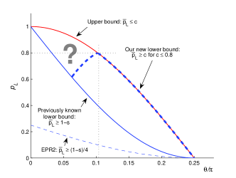
Figure 1: Bounds on $\bar{p_{L}}(\theta)$ in the EPR2 decomposition for two-qubit pure states, as a function of the state parameter $\theta$. Our new lower bound $\bar{p_{L}}(\theta)\geq\cos 2\theta$, valid for all states such that $\cos 2\theta\leq 0.8$, coincides with the upper bound obtained in Scarani (2008). There is still a gap between the lower and upper bound when $\cos 2\theta>0.8$.

VI Prospects

We thus could prove the conjecture that $\bar{p_{L}}(\theta)=\cos 2\theta$ for all states such that $\cos 2\theta\leq 0.8$. This reinforces our opinion, that the result should indeed hold for all pure two-qubit states.

Unfortunately, we could not find so far an EPR2 decomposition with $p_{L}=\cos 2\theta$ for the very partially entangled states (such that $\cos 2\theta>0.8$). Let us however share a few reflections on how one could possibly look for a suitable local component $P_{L}$, which would allow one to prove the conjecture in full generality.

We realize that our local distribution $P_{L}$ above fails to satisfy the constraints (21) when the state under consideration becomes less and less entangled. In our local model, it might be that we correlated the two parties too strongly, by imposing that they share the same local variable $\vec{\lambda}$.

One idea would be to provide the two parties with two local variables $\vec{\lambda}_{a}$ and $\vec{\lambda}_{b}\in S^{2}$, while still considering response functions of the form $\alpha(\vec{a},\vec{\lambda}_{a})=\mathrm{sign}(a_{z}-\vec{a}\cdot\vec{\lambda}_{a})$ and $\beta(\vec{b},\vec{\lambda}_{b})=\mathrm{sign}(b_{z}-\vec{b}^{\prime}\cdot\vec{\lambda}_{b})$. Instead of imposing $\vec{\lambda}_{a}=\vec{\lambda}_{b}$ as in our previous model, we would correlate $\vec{\lambda}_{a}$ and $\vec{\lambda}_{b}$ in a smoother way, depending on the state we consider. In the extreme cases, we would still impose $\vec{\lambda}_{a}=\vec{\lambda}_{b}$ for the maximally entangled state ($\theta=\frac{\pi}{4}$), while the two $\vec{\lambda}$’s would be completely decorrelated for the product state ($\theta=0$).

The problem is now to find the proper way to correlate the two $\vec{\lambda}$’s for each state, i.e. determine the distribution functions $\rho_{\theta}(\vec{\lambda}_{a},\vec{\lambda}_{b})$. Here are a few properties that we might want to impose on $\rho_{\theta}(\vec{\lambda}_{a},\vec{\lambda}_{b})$:

• Forgetting about $\vec{\lambda}_{b}$, $\vec{\lambda}_{a}$ should be uniformly distributed, and vice versa. This will ensure in particular that the marginals are those expected: $M_{L}(\vec{a})=a_{z},M_{L}(\vec{b})=b_{z}$. One should thus have:

  $${\textrm{for all}}\ \vec{\lambda}_{a},\int\!\!\!\!\!\int_{S^{2}}\!\mathrm{d}\!\lambda_{b}\rho_{\theta}(\vec{\lambda}_{a},\vec{\lambda}_{b})=\frac{1}{4\pi}\ ;$$ (35)

  $${\textrm{for all}}\ \vec{\lambda}_{b},\int\!\!\!\!\!\int_{S^{2}}\!\mathrm{d}\!\lambda_{a}\rho_{\theta}(\vec{\lambda}_{a},\vec{\lambda}_{b})=\frac{1}{4\pi}\ .$$ (36)

• Let us denote by ($\vartheta_{a(b)}$,$\varphi_{a(b)}$) the spherical coordinates of $\vec{\lambda}_{a(b)}$. It looks very natural to impose that $\rho_{\theta}(\vec{\lambda}_{a},\vec{\lambda}_{b})$ should only depend on $\vartheta_{a},\vartheta_{b}$ and $\varphi=\varphi_{b}-\varphi_{a}$, that it should be symmetrical when exchanging $\vec{\lambda}_{a}$ and $\vec{\lambda}_{b}$, and that it should have an even dependence on $\varphi$:

  $$\rho_{\theta}(\vec{\lambda}_{a},\vec{\lambda}_{b}) = \rho_{\theta}(\vartheta_{a},\vartheta_{b},\varphi)$$ (37)

  $$= \rho_{\theta}(\vartheta_{b},\vartheta_{a},\varphi)$$ (38)

  $$= \rho_{\theta}(\vartheta_{a},\vartheta_{b},-\varphi)\ .$$ (39)

• According to an argument presented in Appendix B, not all pairs $(\vec{\lambda}_{a},\vec{\lambda}_{b})$ should be allowed. More precisely, writing $c_{a}=\cos\frac{\vartheta_{a}}{2},s_{a}=\sin\frac{\vartheta_{a}}{2},c_{b}=\cos\frac{\vartheta_{b}}{2},s_{b}=\sin\frac{\vartheta_{b}}{2}$ and $c_{\varphi}=\cos\varphi$, one should have

  $$\rho_{\theta}(\vec{\lambda}_{a},\vec{\lambda}_{b})=0\quad\textrm{if}\quad\frac{s_{a}s_{b}}{1-c_{a}c_{b}c_{\varphi}}<s\ .$$ (40)

We therefore suggest the following research program, to prove the above conjecture for all states: find candidate functions $\rho_{\theta}(\vec{\lambda}_{a},\vec{\lambda}_{b})$ that have the previous desired properties (36–40), and then check whether the induced local probability distributions $P_{L}$ satisfy the constraints (21). If one can find such solutions, then this will prove that $\bar{p_{L}}(\theta)=\cos 2\theta$ indeed holds for all two-qubit pure states. On the other hand, if it turned out to be impossible to find such a function, then we might need to change our local model, and maybe relax the assumption that the non-local part should have random marginals.

VI.1 Acknowledgements

We are grateful to Antonio Acín, Mafalda Almeida, Jean-Daniel Bancal, Nicolas Brunner, Loren Coquille, Marc-André Dupertuis, Alexandre Fête and Stefano Pironio for stimulating discussions.

This work is supported by the Swiss NCCR Quantum Photonics, the European ERC-AG QORE, and the National Research Foundation and Ministry of Education, Singapore.

Appendix A: Calculation of $E_{L}(\vec{a},\vec{b})$

Here we calculate the correlation coefficient $E_{L}(\vec{a},\vec{b})$ for our local probability distribution $P_{L}$:

$$E_{L}(\vec{a},\vec{b})$$

$$\quad=\int\!\!\!\!\!\int_{S^{2}}\frac{\mathrm{d}\!\lambda}{4\pi}\ \mathrm{sign}(a_{z}-\vec{a}\cdot\vec{\lambda})\ \mathrm{sign}(b_{z}-\vec{b}^{\prime}\cdot\vec{\lambda})$$

$$\quad=\int\!\!\!\!\!\int_{S^{2}}\frac{\mathrm{d}\!\lambda}{4\pi}\ \big{(}1-2[\vec{a}\cdot\vec{\lambda}\geq a_{z}]\big{)}\ \big{(}1-2[\vec{b}^{\prime}\cdot\vec{\lambda}\geq b_{z}]\big{)}$$

$$\quad=a_{z}+b_{z}-1+\frac{1}{\pi}\int\!\!\!\!\!\int_{S^{2}}\mathrm{d}\!\lambda\ [\vec{a}\cdot\vec{\lambda}\geq a_{z}]\ [\vec{b}^{\prime}\cdot\vec{\lambda}\geq b_{z}],$$

(41)

where $[\cdot]$ is the logical value of what is inside the brakets. The integral represents the area of the intersection of two spherical caps centered around $\vec{a}$ and $\vec{b}^{\prime}$, and tangent to the north pole of the Bloch sphere.

Let us parameterize $\vec{\lambda}\in S^{2}$ by its zenithal and azimuthal angles $(\vartheta,\varphi)$, where $\varphi$ is defined (for simplicity) with respect to the vertical half-plane that contains $\vec{a}$. As $E_{L}(\vec{a},\vec{b})$ should not depend on the sign of $\chi$ (the difference between the azimuthal angles of $\vec{a}$ and $\vec{b}^{\prime}$), it is sufficient to calculate it for $\chi\geq 0$, and simply replace $\chi$ by $|\chi|$ in the final expression. Also, we assume for now that $\vec{a}$ and $\vec{b}$ are both in the north hemisphere of the sphere.

The two spherical caps can then be defined as

$$\{\vec{\lambda}\ |\ \vec{a}\cdot\vec{\lambda}\geq a_{z}\}$$

$$\quad=\{(\vartheta,\varphi)\ |\ \varphi\in[-\frac{\pi}{2},\frac{\pi}{2}]\ \mathrm{and}\ \vartheta\in[0,\vartheta_{m}^{A}(\varphi)]\}$$

$$\{\vec{\lambda}\ |\ \vec{b}^{\prime}\cdot\vec{\lambda}\geq b_{z}\}$$

$$\quad=\{(\vartheta,\varphi)\ |\ \varphi\in[\chi-\frac{\pi}{2},\chi+\frac{\pi}{2}]\ \mathrm{and}\ \vartheta\in[0,\vartheta_{m}^{B}(\varphi)]\}$$

with $\vartheta_{m}^{A}(\varphi),\vartheta_{m}^{B}(\varphi)\in[0,\pi]$ such that

$$\cos\vartheta_{m}^{A}(\varphi) = \frac{a_{z}^{2}-a_{\perp}^{2}\cos^{2}\varphi}{a_{z}^{2}+a_{\perp}^{2}\cos^{2}\varphi}\ ,$$

$$\cos\vartheta_{m}^{B}(\varphi) = \frac{b_{z}^{2}-b_{\perp}^{2}\cos^{2}(\varphi-\chi)}{b_{z}^{2}+b_{\perp}^{2}\cos^{2}(\varphi-\chi)}\ .$$

Let us define $\varphi_{0}$ as the azimuthal angle for which $\vartheta_{m}^{A}(\varphi_{0})=\vartheta_{m}^{B}(\varphi_{0})$. The integral in (41) can then be calculated as follows:

$$\int\!\!\!\!\!\int_{S^{2}}\mathrm{d}\!\lambda\ [\vec{a}\cdot\vec{\lambda}\geq a_{z}]\ [\vec{b}^{\prime}\cdot\vec{\lambda}\geq b_{z}]$$

$$\qquad=\int_{\chi-\pi/2}^{\pi/2}\mathrm{d}\varphi\int_{0}^{\min(\vartheta_{m}^{A}(\varphi),\vartheta_{m}^{B}(\varphi))}\sin\vartheta\mathrm{d}\vartheta$$

$$\qquad=\int_{\chi-\pi/2}^{\varphi_{0}}\mathrm{d}\varphi\big{[}1-\cos\vartheta_{m}^{B}(\varphi)\big{]}$$

$$\qquad\quad+\int_{\varphi_{0}}^{\pi/2}\mathrm{d}\varphi\big{[}1-\cos\vartheta_{m}^{A}(\varphi)\big{]}\ .$$

Using the antiderivative $\int\!\mathrm{d}\varphi\frac{a_{z}^{2}-a_{\perp}^{2}\cos^{2}\varphi}{a_{z}^{2}+a_{\perp}^{2}\cos^{2}\varphi}=2a_{z}\arctan(a_{z}\tan\varphi)-\varphi$, we find:

$$\int\!\!\!\!\!\int_{S^{2}}\mathrm{d}\!\lambda\ [\vec{a}\cdot\vec{\lambda}\geq a_{z}]\ [\vec{b}^{\prime}\cdot\vec{\lambda}\geq b_{z}]$$

$$\qquad\qquad=2\pi-2\chi+2a_{z}\arctan(a_{z}\tan\varphi_{0})-\pi a_{z}$$

$$\qquad\qquad\qquad+2b_{z}\arctan(b_{z}\tan(\chi-\varphi_{0}))-\pi b_{z}\ .$$

(42)

We note that $\vartheta_{m}^{A}(\varphi_{0})=\vartheta_{m}^{B}(\varphi_{0})$ implies $a_{z}b_{\perp}\cos(\chi-\varphi_{0})=a_{\perp}b_{z}\cos\varphi_{0}$, which in turn implies $\ a_{z}\tan\varphi_{0}=\frac{a_{\perp}b_{z}-a_{z}b_{\perp}\cos\chi}{b_{\perp}\sin\chi}\$ and $\ b_{z}\tan(\chi-\varphi_{0})=\frac{a_{z}b_{\perp}-a_{\perp}b_{z}\cos\chi}{a_{\perp}\sin\chi}\$. Inserting these values in (42), then inserting the integral in (41) and writing $|\chi|$ instead of $\chi$, we get the correlation coefficient:

$$E_{L}(\vec{a},\vec{b}) = 1-\frac{2|\chi|}{\pi}+\frac{2}{\pi}a_{z}\arctan(\frac{a_{\perp}b_{z}-a_{z}b_{\perp}\cos\chi}{b_{\perp}\sin|\chi|})$$

$$\qquad\qquad+\frac{2}{\pi}b_{z}\arctan(\frac{a_{z}b_{\perp}-a_{\perp}b_{z}\cos\chi}{a_{\perp}\sin|\chi|})\ .$$

So far we have calculated this coefficient for settings in the north hemisphere of the Bloch sphere. If the settings are in the south hemisphere, one can use the fact that $E_{L}(\vec{a},\vec{b})=-E_{L}(\vec{a},-\vec{b})=-E_{L}(-\vec{a},\vec{b})=E_{L}(-\vec{a},-\vec{b})$. One can check that the above expression is actually still valid for all cases.

Note finally that in the above calculation, we didn’t pay attention to particular cases, when the denominators in the fractions would be zero. For $\chi=0$ or $\pi$, $E_{L}$ (as in eq (31)) can be obtained by taking the corresponding limit in the previous expression, or can be obtained directly in a much simpler way.

Appendix B: Allowed pairs ($\vec{\lambda}_{a},\vec{\lambda}_{b}$) in our last proposal

Here we will argue that in our last proposal with two different local variables $\vec{\lambda}_{a}$ and $\vec{\lambda}_{b}$ for Alice and Bob, not all pairs ($\vec{\lambda}_{a},\vec{\lambda}_{b}$) should be allowed.

The argument is based on the following observation: suppose that Alice measures along direction $\vec{a}=(a_{\perp}\cos\varphi_{a},a_{\perp}\sin\varphi_{a},a_{z})$, and finds the outcome $\alpha=+1$; this projects Bob’s state onto $\mbox{$\langle+\vec{a}|$}\otimes\mathbbm{1}\ \mbox{$|\psi(\theta)\rangle$}=\sqrt{\frac{1+ca_{z}}{2}}\mbox{$|\vec{b}_{\vec{a}}\rangle$}$, with $\vec{b}_{\vec{a}}=(\frac{sa_{\perp}}{1+ca_{z}}\cos\varphi_{a},-\frac{sa_{\perp}}{1+ca_{z}}\sin\varphi_{a},\frac{c+a_{z}}{1+ca_{z}})$. If Bob then measures the setting $\vec{b}_{\vec{a}}$, he will necessarily get the result $\beta=+1$, and therefore

$$P_{Q}(+-|\vec{a},\vec{b}_{\vec{a}})=0.$$

This in turn implies, for the EPR2 decomposition $P_{Q}=p_{L}P_{L}+(1-p_{L})P_{NL}$ (with $p_{L}\neq 0$), that

$$P_{L}(+-|\vec{a},\vec{b}_{\vec{a}})=0.$$

This constraint must be satisfied by any setting $\vec{a}$ (which defines the setting $\vec{b}_{\vec{a}}$). To ensure this, we shall not allow pairs $(\vec{\lambda}_{a},\vec{\lambda}_{b})$ that may give the results $(\alpha=+1,\beta=-1)$, for some choice of settings of the form $(\vec{a},\vec{b}_{\vec{a}})$.

To make this more explicit, let us fix the first local variable $\vec{\lambda}_{a}$. For simplicity, we assume that $\vec{\lambda}_{a}$ is in the $xz$ plane. If this is not the case, the analysis below would be slightly more tedious, but the final result would be the same.

The settings $\vec{a}$ that give the result $\alpha(\vec{a},\vec{\lambda}_{a})=+1$ span the half-sphere $\cal{A}$ above the bisector plane between $\vec{z}$ and $\vec{\lambda}_{a}$; see Figure 2 (left) for a 2D representation. $\cal{A}$ can be defined as

$${\cal A}=\{\vec{a}|\vec{u}\cdot\vec{a}\geq 0\},\quad\mathrm{where}\ \ \vec{u}=(-c_{a},0,s_{a}).$$

(Let us recall the notations: ($\vartheta_{a(b)}$,$\varphi_{a(b)}$) are the spherical coordinates of $\vec{\lambda}_{a(b)}$, and we write $c_{a}=\cos\frac{\vartheta_{a}}{2},s_{a}=\sin\frac{\vartheta_{a}}{2},c_{b}=\cos\frac{\vartheta_{b}}{2},s_{b}=\sin\frac{\vartheta_{b}}{2}$ and $c_{\varphi}=\cos(\varphi_{b}-\varphi_{a})$.)

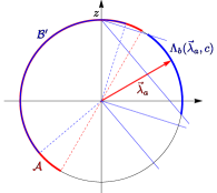
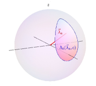
Figure 2: Construction of the set $\Lambda_{b}(\vec{\lambda}_{a},c)$ of allowed local variables $\vec{\lambda}_{b}$, given the first variable $\vec{\lambda}_{a}$. Left: 2D cut in the vertical plane that contains $\vec{\lambda}_{a}$. Right: 3D representation of $\Lambda_{b}(\vec{\lambda}_{a},c)$. For both figures, $\vartheta_{a}=\frac{\pi}{3}$, $c=0.5$.

The settings $\vec{b}_{\vec{a}}$, corresponding to these settings $\vec{a}\in\cal{A}$, then also span a spherical cap, $\cal{B}$, included in $\cal{A}$. Using the fact that $a_{z}=\frac{(b_{\vec{a}})_{z}-c}{1-c(b_{\vec{a}})_{z}}$ and $a_{\perp}=\frac{s(b_{\vec{a}})_{\perp}}{1-c(b_{\vec{a}})_{z}}$, $\cal{B}$ can in turn be defined as

$${\cal B}=\{\vec{b}_{\vec{a}}|\vec{u}\cdot\vec{a}\geq 0\}=\{\vec{b}|-\vec{v}\cdot\vec{b}\geq cs_{a}\},$$

$$\mathrm{where}\ \ \vec{v}=(sc_{a},0,-s_{a}).$$

According to the above observation, the allowed local variables $\vec{\lambda}_{b}$ must be such that for all those settings $\vec{b}_{\vec{a}}$ in $\cal{B}$, $\beta(\vec{b}_{\vec{a}},\vec{\lambda}_{b})\neq-1$, i.e., $(\vec{\lambda}_{b}-\vec{z})\cdot\vec{b}_{\vec{a}}^{\prime}\leq 0$. This implies that $\vec{\lambda}_{b}-\vec{z}$ should be in a cone centered around $\vec{v}$, and with a half-angle $\xi=\arcsin\frac{cs_{a}}{||\vec{v}||}$. This writes

$$\vec{v}\cdot\frac{\vec{\lambda}_{b}-\vec{z}}{||\vec{\lambda}_{b}-\vec{z}||}\geq||\vec{v}||\cos\xi=s\,.$$

For the fixed $\vec{\lambda}_{a}$ considered here, the set of allowed variables $\vec{\lambda}_{b}$ is then the intersection of this cone, translated by $\vec{z}$, and the Bloch sphere; see Figure 2. Writing $\vec{\lambda}_{b}=(2c_{b}s_{b}c_{\varphi},2c_{b}s_{b}s_{\varphi},1-2s_{b}^{2})$, the previous condition implies, that:

$$\mathrm{the\ pair\ }(\vec{\lambda}_{a},\vec{\lambda}_{b})\ \mathrm{should\ be\ allowed\ only\ if\ \ }\frac{s_{a}s_{b}}{1-c_{a}c_{b}c_{\varphi}}\geq s\ .$$

This justifies the constraint (40).

References

- Bell (1964) J. S. Bell, Physics 1, 195 (1964).
- Elitzur et al. (1992) A. C. Elitzur, S. Popescu, and D. Rohrlich, Phys. Lett. A 162, 25 (1992).
- Scarani (2008) V. Scarani, Phys. Rev. A 77, 042112 (2008).
- Barrett et al. (2006) J. Barrett, A. Kent, and S. Pironio, Phys. Rev. Lett. 97, 170409 (2006).
- Zhang et al. (2009) F. Zhang, C. Ren, M. Shi, and J. Chen, arXiv:0909.1634 (2009).
- Brunner et al. (2008) N. Brunner, N. Gisin, S. Popescu, and V. Scarani, Phys. Rev. A 78, 052111 (2008).
- Pearle (1970) P. M. Pearle, Phys. Rev. D 2, 1418 (1970).
- Braunstein and Caves (1990) S. L. Braunstein and C. M. Caves, Ann. Phys. 202, 22 (1990).
- Scarani (2007) V. Scarani, arXiv:0712.2307v1 (2007), early version of Scarani (2008).
- Barrett and Pironio (2005) J. Barrett and S. Pironio, Phys. Rev. Lett. 95, 140401 (2005).
- Jones and Masanes (2005) N. S. Jones and L. Masanes, Phys. Rev. A 72, 052312 (2005).
- Bell (1966) J. S. Bell, Rev. Mod. Phys. 38, 447 (1966).