How well can the LHC distinguish between the SM light Higgs scenario, a composite Higgs and the Higgsless case using VV scattering channels?
Abstract:
A complete parton level analysis of + four jets () and + two jets production at the LHC is presented, including all processes at order , and when appropriate. The infinite Higgs mass scenario, which is considered as a benchmark for strong scattering theories and is the limiting case for composite Higgs models, and one example of a model incorporating a Strongly Interacting Light Higgs are confronted with the Standard Model light Higgs predictions. This analysis is combined with the results in the + four jets channel presented in a previous paper, in order to determine whether a composite Higgs signal can be detected as an excess of events in boson–boson scattering.
1 Introduction
The Standard Model (SM) describes Electroweak Symmetry Breaking (EWSB) in the most simple and economical fashion through a single complex Higgs doublet, with only a neutral scalar field in the spectrum. The fit of EW precision data is in agreement with the SM predictions to an unprecedented accuracy and gives an upper limit on the Higgs mass of about 182 GeV [1]. Direct searches at LEP2 imply [2] while, more recently D0 and CDF at the Tevatron have excluded at 95%CL a SM Higgs in the range [3]. The LHC will have the task to reveal whether this minimal realization of EWSB takes place in Nature or a more complex structure is present111 Detailed reviews and extensive bibliographies can be found in Refs. [4, 5, 6, 7, 8].
If the Higgs field is not found, scattering processes between longitudinally polarized vector bosons will play a prominent role because, without a Higgs, the corresponding amplitudes grow with energy and violate perturbative unitarity at about one TeV [9], requiring new physics in the energy range accessible to the LHC.
Many alternative mechanisms of EWSB have been explored. We will not try to summarize the different models and simply refer to the literature. For our purpose we will only remark that it is conceivable and widely discussed [10, 11, 12, 13, 14, 15, 16] that composite states are responsible for EWSB as nicely recently reviewed in Ref. [17]. These theories are characterized by the presence of new states which could be produced at the LHC, if light enough.
In view of the large number of different proposals it is useful to determine the model independent features of this class of theories. There has been recent progress in this area [18, 19, 20], using the effective theory language [21]. In Ref. [19] it has been pointed out that, if EWSB is triggered by a light composite Higgs which is a pseudo–Goldstone boson related to some large scale strongly interacting dynamics, the growth with energy of the vector boson scattering amplitudes typical of Higgsless models might not be completely canceled by Higgs exchange diagrams but only slowed down because of the modified couplings between the Higgs field and the vector bosons with respect to the SM ones. Such a Higgs has been called Strongly Interacting Light Higgs (SILH). If the mass of the Higgs boson becomes larger than the typical energy scale at which boson–boson scattering is probed, the contribution of the Higgs exchange diagrams decreases and completely vanishes, in the Unitary gauge we employ throughout our calculation, in the limit of an infinite mass which we will refer to as the Higgsless case. As a consequence, the scattering cross section for an infinitely massive Higgs in the SM represents, at large energies, an upper limit for VV scattering processes in SILH models, and can be taken as a benchmark for the observability of signals of strong scattering and of Higgs compositeness in boson–boson reactions. On the other hand the Higgsless case is also representative of models in which heavy resonances which unitarize boson–boson scattering are present but cannot be directly detected at the LHC.
Scattering processes among vector bosons have been scrutinized since a long time [22, 23]. In Ref. [24, 25] an analysis of + four jets and + four jets production at the LHC has been presented, with the limitation of taking into account only purely electroweak processes. Preliminary results concerning the inclusion of the background, which include and top–antitop production have appeared in Ref. [26]. A preliminary analysis in the Equivalent Vector Boson Approximation of the observability of partial unitarization of longitudinal vector boson scattering in SILH models at the LHC can be found in Ref. [27]. In the last few years QCD corrections to boson–boson production via vector boson fusion [28] at the LHC have been computed and turn out to be below 10%. Recently, VBFNLO [29] a Monte Carlo program for vector boson fusion, double and triple vector boson production at NLO QCD accuracy, limited to the leptonic decays of vector bosons, has been released.
In Ref. [30] a complete parton level analysis of + four jets production at the LHC, including all processes at order , and has been presented, comparing a typical SM light Higgs scenario with the Higgsless case. It was noted that the + 4j background is so large to make the usual approach of comparing the number of events in the two scenarios at large invariant masses rather ineffective. An alternative strategy was suggested, namely to focus on the invariant mass distribution of the two central jets which is characterized by a peak corresponding to the decays of vector bosons which is present in the vector–vector scattering signal and by an essentially flat background produced by processes. The latter can be measured from the sidebands drastically decreasing the theoretical uncertainties. In Ref. [30] the probability of observing a signal of new physics in the channel was estimated constructing the probability distribution of experimental results both in the SM and in the Higgsless case, taking into account the statistical uncertainties for both signals and background and the theoretical uncertainty for the signal alone, assuming that the background can be extrapolated from the measured sidebands. The probability that the benchmark Higgsless scenario would result in an experimental outcome outside the SM 95% exclusion limit, assuming a 200 fb-1 luminosity for both the muon and electron decay channel, turned out to be about 97%.
In this paper we complete our study examining at parton level the processes and , including all irreducible backgrounds contributing to these six parton final states. These are the only vector–vector scattering reactions, together with mentioned above, in which the presence of at least one pair of leptons in the final state ensures a sufficiently clean determination of the invariant mass of the outgoing vector bosons, up to the ambiguity related to the momentum reconstruction of the unobserved neutrino. The latter can be however be estimated by imposing the condition that the missing momentum and the charged lepton reconstruct the W mass. It is here implied that the channel, while allowing a more precise reconstruction of the mass, has a negligible rate at the LHC at large invariant masses of the four-lepton system due to the small branching ratio of the leptonic decays. The invariant mass of the two outgoing bosons is the analogue of the center–of–mass energy for on–shell vector boson scattering: differences between the Higgsless scenario and the SM predictions increase, for the processes we analyze, with the boson pair invariant mass.
In this paper we consider three scenarios: a light Higgs SM framework with GeV, one instance of the SILH models which we will describe shortly and an infinite mass Higgs scenario. We combine the results for and with those obtained in Ref. [30] for the channel in order to obtain a global estimate, including all three channels, of the probability of distinguishing the considered Beyond Standard Model (BSM) cases from the SM scenario.
2 The Strongly Interacting Light Higgs scenario
The effective field theory approach [21] is a powerful tool for describing the low energy dynamics of systems with broken symmetries. It provides a systematic expansion of the full unknown Lagrangian in terms of the fields which are relevant at scales much lower than the symmetry breaking scale. In Ref. [19] this general framework has been employed to describe the main features of the models of EWSB in which the Higgs field can be identified with a pseudo–Goldstone boson of some broken strong interaction at high energy. Models which fall into this class are for instance the Holographic Higgs [15], the Little Higgs of Ref. [16] and the Littlest Higgs [12].
These theories generally predict new resonances and their search may well be the best way to detect New Physics effects at the LHC. However they also lead to modifications of boson–boson scattering which might provide further evidence and possibly be the only accessible effects if the new resonances are heavy.
The leading low energy effects are described by two parameters (one responsible for a universal modification of all Higgs couplings, and the other one for a universal modification of Higgs couplings to fermions) characterized by the ratio , where is the Higgs vacuum expectation value and is the –model scale. The natural range of the parameter is between and which correspond respectively to the limiting cases of the Standard Model and of technicolor theories. Because of the modified Higgs couplings, longitudinal gauge–boson scattering amplitudes violate unitarity at high energy, even in the presence of a light Higgs [19]. The –growing amplitude is typically smaller than in the Higgsless case and the violation is moved to a larger energy regime.
Therefore, even if a light Higgs is discovered, boson–boson scattering is a crucial process to study and can give us useful information on the nature of the Higgs boson. It is worth pointing out that, in this framework, since the Higgs can be viewed as an approximate fourth Goldstone boson, its properties are related to those of the exact (eaten) Goldstone bosons. Strong gauge–boson scattering will be accompanied by strong Higgs pair production [19].
The effective Lagrangian approach of Ref. [19] is valid for small values of , while larger values demand a more detailed description of the particular model at hand. Such a Lagrangian leads to a modification of the Higgs couplings by a factor , which can be reabsorbed in a Higgs propagator modification by a factor in boson boson scattering studies. is a pure number of order unity [12, 15, 16, 19]. For the present study we have selected the value which we intend as a possible upper limit for the model independent lagrangian description of Ref. [19].
3 Outline of the analysis
The observation of strong boson–boson scattering as an excess of events compared to the SM prediction requires, as an essential condition, that a signal of VV scattering is extracted from the background. At the same time the selection strategy must be capable to maximize the differences between the light Higgs and the BSM cases.
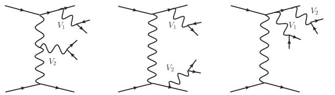
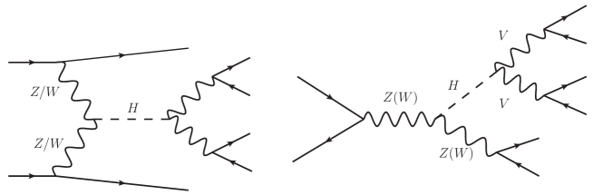
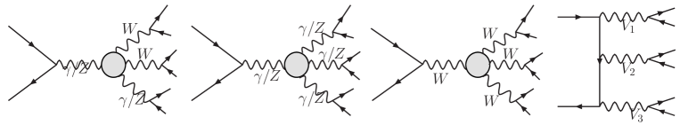
Three(two) perturbative orders contribute to the background for () final states. At there are a large number of diagrams which cannot be interpreted as boson–boson scattering and which cannot be separated in any sensible way from the scattering type diagrams due to large cancellations between the two sets [25]. For illustrative purpose a number of diagrams are shown in Figs. 1–6. Fig. 1 illustrates the class of diagrams which include boson–boson scattering subdiagrams while Fig. 2 presents some representative diagrams in which two vector bosons are produced but no fusion takes place. Fig. 3 and Fig. 4 show diagrams which describe Higgs production and three vector boson production.
At we have to deal with the production of two electroweak bosons plus two jets without any scattering contribution. Some representative diagrams are shown in Fig. 5 which also includes diagrams describing production which contribute only to the channel. For the final state there are contributions at in which only one electroweak boson is effectively produced, while the additional jets, which, taken in pairs, do not peak at any particular mass, populate the full available phase space with a production rate which is much larger than the signal one. A few diagrams in this set are presented in Fig. 6.
The first step is concerned with the identification of a suitable kinematic signature which allows to capture the essence of scattering. The selection of events widely separated in pseudorapidity is a well established technique for enhancing the scattering contributions at the LHC [22, 23]. Looking at the topology of the diagrams embedding the gauge boson scattering as a subprocess, one concludes that it is appropriate to associate the two most forward/backward jets to the tag quarks which radiate the bosons which initiate scattering. As shown in Ref. [30] a powerful tool to increase the separation between the SM predictions and those of the Higgsless scenario is provided, at large invariant masses, by the request that the vector bosons and their decay products are in the central part of the detector since the vector bosons in the Higgsless case have smaller rapidities and larger momenta than in the presence of a light Higgs. The main purpose of this kinematic selection is to isolate a sample of genuine events while suppressing the contribution of irreducible backgrounds such as three boson production or top quark production.
Having isolated a sample of candidate scattering events, one needs to define an observable quantity which is as susceptible as possible to the details of the mechanism of EWSB in order to maximize the sensitivity to effects of alternative models such as strong scattering. For the channel this task is straightforward only apparently. As already mentioned, the QCD background is expected to provide a significant number of fake events as a consequence of the large cross section. The classical approach is to focus on the invariant mass distribution of the final state boson pair. The huge QCD background, with its large scale uncertainty, makes this procedure rather dubious for the case. Detecting signals of EWSB in the vector pair mass distribution remains a formidable challenge. The analysis of Ref. [30] shows that, even focusing the attention on the high invariant vector pair mass region and requiring the mass of the two central jets to be close to the mass of a vector boson, the expected signal over background ratio is of the order of 1/10. This way of measuring the signal, typical of a counting experiment, finds a substantial obstacle in the spread of the interesting excess of events over a wide region in .
A possible way out for this problem is to look instead at the invariant mass of the two central jets () for events with large vector pair mass. Provided a convenient set of kinematic cuts has been applied, the + cross section is dominated by the peaks corresponding to and decays to quarks, while the contribution is non–resonant in this respect. When restricting to the window between 70 and 100 GeV, which covers completely the and resonances, we find that the distribution is essentially flat and therefore can reliably be measured from the sidebands of the physical region of interest. This procedure has several advantages. On one side, it eliminates the theoretical uncertainty associated with the scale dependence of the contribution. On the other side, it allows to subtract the dominant contribution to the irreducible QCD background, enhancing the visibility of genuine EWSB effects. The signal has a very clear signature, a bump in the two central jet mass distribution, which is much easier to hunt for experimentally than a diffuse excess in production cross section.
Once the non–resonant background has been subtracted, one is left with a peak whose size is strictly related to the regime of the EWSB dynamics: a strongly–coupled scenario would result in a more prominent peak than a weakly–coupled one. This feature suggests to take the integral of the peak as the discriminator among different models. At a given collider luminosity, the number of expected events can be derived. With a slight abuse of language, we call this number the VBS signal. It is by analyzing the probability density function (p.d.f.) associated with this discriminator that we can determine, in the last step, the confidence level for a given experimental result to be or not to be SM–like, in the same spirit of the statistical procedure adopted for the search of the Standard Model Higgs boson at LEP [31].
For the channel the physical picture is straightforward, the invariant mass of the vector boson pair can be directly measured from the momenta of the charged leptons and the reconstructed neutrino momentum. Since the background is much smaller than in the case we use the total expected number of events as discriminator and estimate the probability that the experimental results in the BSM models are incompatible with the SM.
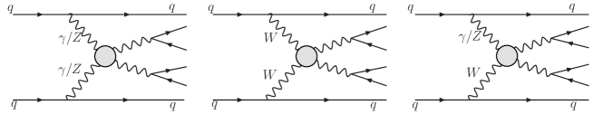
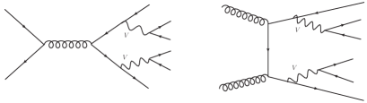
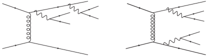
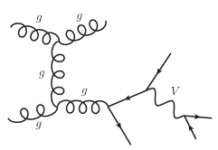
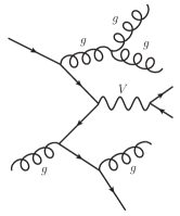
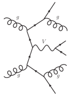
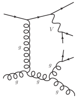
Representative Feynman diagrams for the ,
production processes at the LHC.
4 Calculation
As discussed in Sect. 3, three perturbative orders contribute to at the LHC, while only two perturbative orders contribute to . The and samples have been generated with PHANTOM, a dedicated tree level Monte Carlo generator which is documented in Ref. [32] while additional material can be found in Refs. [33, 34, 35]. The sample has been produced with MADEVENT [36]. Both programs generate events in the Les Houches Accord File Format [37]. In all samples full matrix elements, without any production times decay approximation, have been used. For the LHC we have assumed the design energy of 14 TeV. For each perturbative order we have generated a sample of five hundred thousand unweighted events.
For the Standard Model parameters we use the input values:
| (1) |
The masses of all other partons have been set to zero. We adopt the standard –scheme to compute the remaining parameters.
All samples have been generated using CTEQ5L [38] parton distribution functions. For the and samples, generated with PHANTOM, the QCD scale has been taken as:
| (2) |
while for the sample the scale has been set to . This difference in the scales conservatively leads to a definite relative enhancement of the background. Tests in comparable reactions at have shown an increase of about a factor of 1.5 for the processes computed at with respect to the same processes computed with the larger scale Eq.(2).
We work at parton level with no showering and hadronization. The two jets with the largest and smallest rapidity are identified as forward and backward tag jet respectively. The two intermediate jets called central and are considered as candidate vector boson decay products.
The neutrino momentum is reconstructed according to the usual prescription, requiring the invariant mass of the pair to be equal to the boson nominal mass,
| (3) |
in order to determine the longitudinal component of the neutrino momentum.
For very large Higgs masses, all Born diagrams with Higgs propagators become completely negligible in the Unitary Gauge we work in. Therefore the Higgsless model results for all processes coincide with those in the limit.
The cuts in Tab. 1 have been applied either at generation level or as a preliminary step to any further analysis. They require containment within the active region of the detectors and minimum transverse momentum for all observed partons; a minimum mass separation is imposed for all same–family opposite–sign charged leptons, while a minimum separation both in mass and in is required for jet pairs. At large transverse momentum, jet pairs with mass comparable to the mass of electroweak bosons or even larger can merge into one single jet when an angular measure like is adopted for reconstructing jets. Therefore we have imposed that all partons satisfy , a value smaller than usually employed in LHC analyses. However, in Sect. 8 we discuss in more detail the effect of removing the angular separation constraint or, on the contrary, of imposing a more stringent requirement . Furthermore, the most forward and most backward jets are required to be separated by at least four units in rapidity and their combined mass is forced to be outside the electroweak vector boson mass window; on the contrary the mass of the two remaining jets, which we will call central in the following, is required to be compatible with the mass of the weak bosons; no () triplet is allowed in the neighborhood of the top mass for the () channel.
| Acceptance cuts |
|---|
| () |
| () |
5 The channel
The total cross section for the channel with the generation cuts in Tab. 1 is presented in Tab. 2 as a function of the minimum invariant mass for the system. These results refer to the mass window and include all three perturbative orders. In parentheses the results for the sum of the and processes. Tab. 2 shows that the cross section is dominated by the contribution. If we assume a luminosity of and sum over the electron and muon channels the difference between the number of events expected for an infinite mass Higgs and a light one is smaller than the expected statistical uncertainty for the processes and no meaningful separation between the two cases can be obtained.
| no Higgs | SILH | GeV | |
| (GeV) | (fb) | (fb) | (fb) |
| 600 | 45.8(1.2) | 45.7(1.06) | 45.6(1.01) |
| 800 | 23.3(0.605) | 23.2(0.515) | 23.2(0.471) |
| 1000 | 12.7(0.318) | 12.6(0.263) | 12.6(0.24) |
| 1200 | 7.15(0.177) | 7.1(0.147) | 7.1(0.134) |
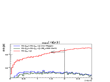
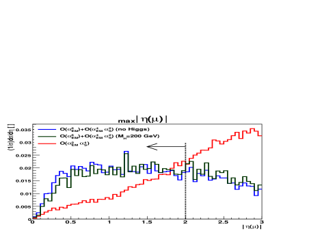
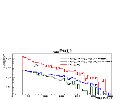
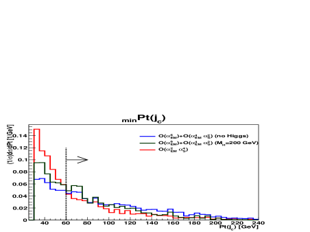
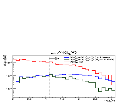
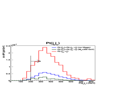
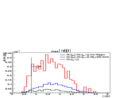
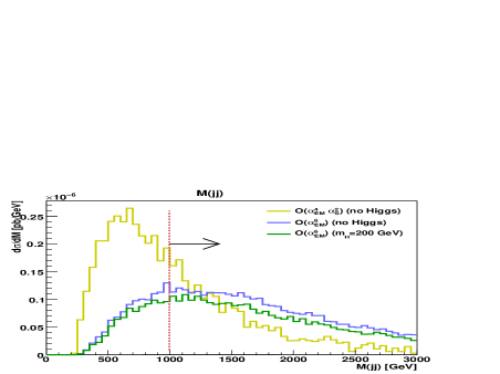
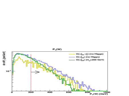
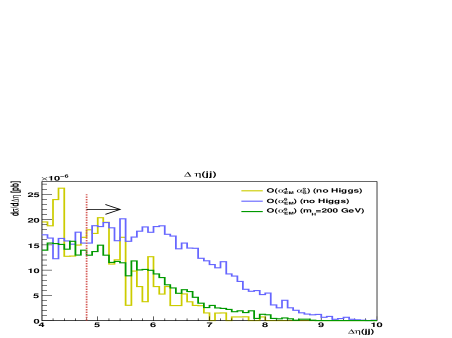
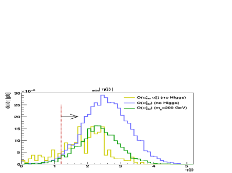
Therefore, on the generated samples we have applied some additional selection cuts. They are shown in Tab. 3 for the channel in the order in which they have been implemented. The corresponding distributions are presented in Figs. 7–9 for the SM and Higgsless cases. In each figure all previous cuts are applied. The vertical dotted line indicates the value of the cut and the arrow indicates which part of the events is kept. For the distribution of the largest absolute pseudorapidity of the charged leptons in Fig. 7 and the distribution of the smallest transverse momentum of the two central jets in Fig. 8 we also present the plots normalized to unit area in order to show more clearly the differences in shape between the different cases.
The essence of the set of cuts in Tab. 3 can be easily understood: they amount to requiring that the two tag jets are highly energetic and well separated both from each other and from the candidate vector bosons; moreover the two reconstructed vector bosons are required to be central and have large transverse momentum.
In Tab. 4 we present the total cross section with the full set of cuts in Tab. 1 and Tab. 3 as the minimum invariant mass for the system is increased between 600 and 1200 GeV. These results refer to the mass window . In parentheses the results for the samples. The last column gives the cross sections for the processes alone; the reported values are computed with the Higgs mass taken to infinity, they agree within statistical errors with those obtained for GeV.
| Selection cuts |
|---|
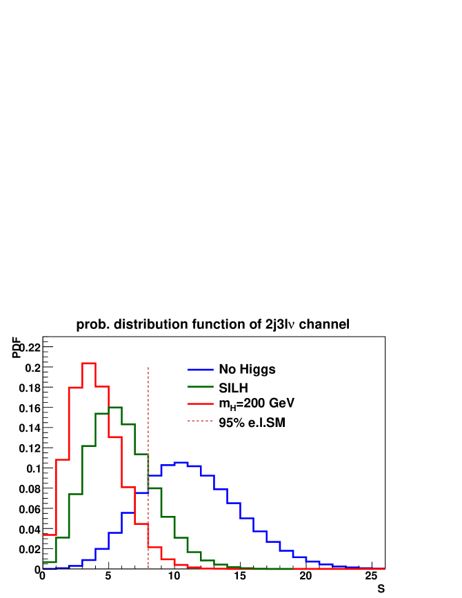
For both the Higgsless and SILH cases we have computed the probability of what we call, for brevity and with a slight abuse of language, the BSM hypothesis at 95% SM exclusion limit, namely the probability that, assuming the absence of a Higgs boson or that the SILH model correctly describes nature, the result of an experimental outcome, with a given luminosity, has a chance of less than 5% in the Standard Model (PBSM@95%CL). For this we proceed as described in Ref. [30], which we briefly summarize for convenience. We define the background as the expected yield of the processes and the signal as the expected number of events from all and processes, both restricted to the mass interval and satisfying all cuts in Tab. 1 and Tab. 3. These contributions correspond respectively to the representative diagrams of Fig. 6 () and Figs. 1–5 (). In other words corresponds to the events which produce a resonant boson peak above the flat background due to in the mass distribution of the two central jets. and are considered as random variables representing the number of background and signal events for a possible experimental outcome. and are the corresponding average values which will be taken equal to the predictions of our simulation for a luminosity and summing over the electron and muon channels. We take into account the statistical uncertainty of both and assuming a standard Poisson distribution with average and respectively. The predicted signal cross section is also affected by theoretical uncertainties, so the parameter is itself subject to fluctuations. For we assume, in addition to the statistical fluctuations, a theoretical error defined as a flat distribution in the window which, in our opinion, is a reasonable choice to account for both pdf’s and scale uncertainties for the signal. The processes we are interested in require center of mass energies of the order of the TeV and therefore involve rather large– quarks, at a typical scale of about 100 GeV. In this region the uncertainty due to the parton distribution functions is of the order of 5% [40, 41]. As already stated, QCD corrections are in the range of 10% and, as a consequence theoretical uncertainties are expected to be well within this order of magnitude. Only statistical fluctuations have been taken into consideration in the case of . This is motivated by the fact that the background is likely to be well measured experimentally from the region outside the signal peak, so that the theoretical error on is not expected to be an issue at the time when real data analysis will be performed. We define the test statistics [39] using the following prescription,
| (4) |
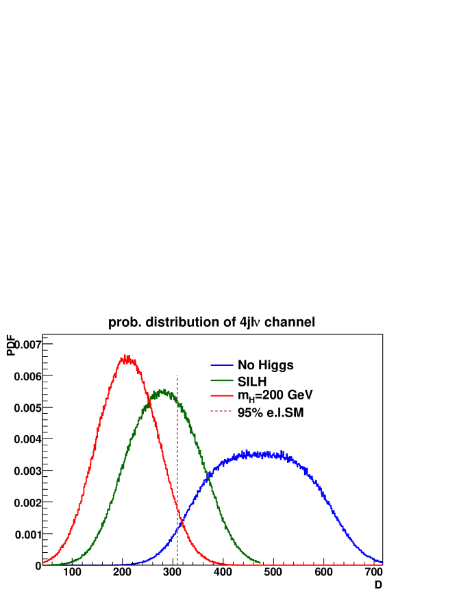
represents the actual number of events found in the peak taking into account statistical fluctuations. The probability distribution of for the three scenarios is reported in Fig. 10 for with the full set of cuts in Tab. 1 and Tab. 3 and under the constraint . The red curve refers to a Higgs of 200 GeV while the green one refers to the SILH model and the blue one to the no–Higgs case. The dotted vertical line in the plot marks the 95% exclusion limit for the SM predictions. We assume a luminosity and sum over the and final states.
| no Higgs | SILH | GeV | ||||
|---|---|---|---|---|---|---|
| (GeV) | (fb) | PBSM | (fb) | PBSM | (fb) | (fb) |
| 600 | 0.705(0.154) | 77.1% | 0.625(0.076) | 16.8% | 0.595(0.0484) | 0.022 |
| 800 | 0.415(0.102) | 75.3% | 0.358(0.0457) | 16.1% | 0.337(0.025) | 0.010 |
| 1000 | 0.209(0.06) | 65.8% | 0.174(0.0245) | 12.3% | 0.162(0.0129) | 0.005 |
| 1200 | 0.117(0.0328) | 44.7% | 0.098(0.0141) | 9.91% | 0.092(0.0077) | 0.003 |
As reported in Tab. 4, the probability of an experiment to find a result incompatible with the SM at 95%CL assuming that the Higgsless model is realized in Nature is of the order of 77% for and decreases to about 45% for . At first sight this is surprising since the difference between the SM and the Higgsless case increases with if only the processes are considered. In fact if for instance one considers the ratio of the Higgsless to the SM cross sections, this can be seen to be larger at higher . This behaviour can however be understood qualitatively in the following way. We can neglect as a first approximation the effect of theory errors which only affects the component. Then, the separation, in terms of events for a luminosity and two lepton channels, between the no–Higgs and the light Higgs case amounts to about 2.5 times the standard deviation of the two distributions for . For however the same separation is about equal to the corresponding standard deviation and therefore the overlap between the two distributions is larger and the statistical discriminating power is reduced. In other terms, the increase of the relative statistical error as the total number of events diminishes at larger is not compensated by the increase of the ratio between the number of genuine scattering events in the Higgsless case compared to the SM one.
For the SILH model the PBSM@95%CL is only about 17% at most, for .
For and summing over the and final states, the expected total rates are about 280/250/240 events for the Higgsless/SILH/SM case for and 47/40/37 for . The background, in the mass window we are focusing on, yields about 220 events for and 33 events for .
6 The channel
The total cross section for the channel with the acceptance cuts in Tab. 1 is presented in Tab. 5 as a function of the minimum invariant mass for the system. In parentheses the results for the processes.
| no Higgs | SILH | GeV | |
| (GeV) | (fb) | (fb) | (fb) |
| 600 | 0.499(0.242) | 0.462(0.213) | 0.452(0.204) |
| 800 | 0.252(0.134) | 0.227(0.114) | 0.219(0.106) |
| 1000 | 0.139(0.078) | 0.122(0.0635) | 0.117(0.0585) |
| 1200 | 0.0815(0.0476) | 0.071(0.0374) | 0.0675(0.0339) |
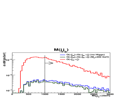
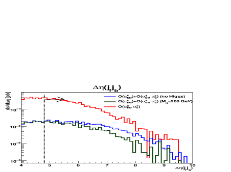
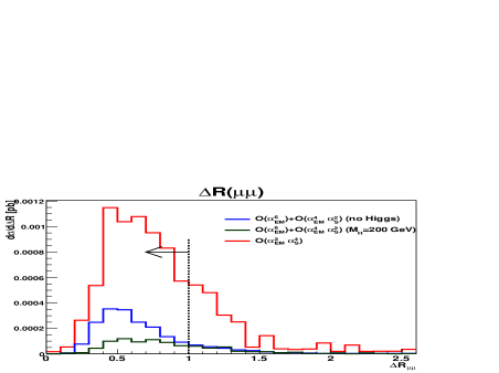
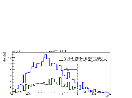
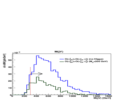
Tab. 5 shows that the cross section for the processes is about equal to the cross section for the contribution. In the following we will consider the full sample as our signal since essentially all events contain a and a boson. It is possible to improve the discriminating power of the analysis increasing the fraction of events in the event sample since only those are sensitive to the mechanism of EWSB. Therefore, on the generated samples we have applied some additional selection cuts. They are shown in Tab. 6 in the order in which they have been implemented. The corresponding distributions are presented in Figs. 11, 12. The vertical dotted line indicates the value of the cut and the arrow indicates which part of the events is kept. The cuts in Tab. 6, as in the case, force the two tag jets to be highly energetic and well separated and the two (reconstructed) vector bosons to be central and to have large transverse momentum.
| Selection cuts |
|---|
The total cross section in attobarns for the channel, with the full set of cuts in Tab. 1 and Tab. 6, as a function of the minimum invariant mass is shown in Tab. 7. In parentheses the results for the contribution are reported. The cross section is dominated by the contribution. The processes including two QCD vertexes give only a small contribution which decreases sharply at larger .

| no Higgs | SILH | GeV | |||
|---|---|---|---|---|---|
| (GeV) | (ab) | PBSM | (ab) | PBSM | (ab) |
| 600 | 26.9(24.8) | 80.0% | 13.5(11.9) | 19.5% | 8.50(6.95) |
| 800 | 18.8(17.8) | 84.1% | 8.20(7.45) | 24.0% | 4.46(3.72) |
| 1000 | 12.8(12.6) | 72.9% | 5.15(4.79) | 15.9% | 2.21(1.83) |
| 1200 | 8.65(8.55) | 65.7% | 3.08(3.00) | 13.1% | 1.19(1.12) |
In Tab. 7 we also give the PBSM@95%CL for the two BSM scenarios. In the present case, since no background is present, we use as discriminant , the sum of the events for all and processes for a luminosity of , summing over the , , and channels. We take into account the statistical uncertainty assuming a standard Poisson distribution and we assume a theoretical error defined as a flat distribution in the window .
The corresponding normalized frequency for the three scenarios is reported in Fig. 13 for . The red curve refers to a Higgs of 200 GeV while the green one refers to the SILH model and the blue one to the no–Higgs case. The dotted vertical line in the plot marks the 95% exclusion limit for the SM predictions.
The probability of an experiment to find a result incompatible with the SM at 95%CL assuming that the Higgsless model is realized in Nature is of the order of 80% and decreases to about 65% for . Because of the absence of large backgrounds this channel has a discriminating power which is in fact higher than the corresponding one for final states. However the expected rates are quite small. Only about ten events are expected for all combinations of muons and electrons for a luminosity of and . It might be extremely difficult to obtain an actual measurement for such a tiny predicted rate once all the experimental efficiencies are folded in and all sources of isolated leptons from the underlying event or from jets faking isolated leptons are taken into account. Clearly this channel would greatly benefit from a larger luminosity. The corresponding probabilities for the SILH model vary between 13% and 25%. In the channel the PBSM@95%CL is somewhat larger at than at smaller value because of the steep decrease of the background at larger .
7 The channel
In this section we recall the results presented in Ref. [30] and complete them with those relative to the SILH model. In addition to the acceptance cuts in Tab. 1 we apply the selection cuts in Tab. 8. The corresponding cross sections are shown in Tab. 9. These results refer to the mass window and include all three perturbative orders. In parentheses the results for the sum of the and processes which we take as our signal as for the channel. The last columns gives the cross sections for the processes alone; the reported values are computed with the Higgs mass taken to infinity, they agree within statistical errors with those obtained for GeV. The PBSM probabilities are obtained using the procedure detailed in Sect. 5.
| Selection cuts |
|---|
| no Higgs | SILH | GeV | ||||
|---|---|---|---|---|---|---|
| (GeV) | (fb) | PBSM | (fb) | PBSM | (fb) | (fb) |
| 600 | 6.07(1.18) | 96.5% | 5.59(0.704) | 35.9% | 5.41(0.524) | 0.23 |
| 800 | 3.76(0.779) | 96.8% | 3.40(0.418) | 29.2% | 3.29(0.309) | 0.13 |
| 1000 | 2.26(0.483) | 95.4% | 2.01(0.227) | 19.8% | 1.94(0.169) | 0.08 |
| 1200 | 1.32(0.263) | 83.9% | 1.19(0.132) | 16.9% | 1.15(0.094) | 0.05 |
For the expected background in the mass window is about 1950 events with a luminosity of and summing over the electron and muon channels. Correspondingly, 209 signal events are expected in the light Higgs SM scenario and 474 in the no Higgs case. The corresponding prediction in the SILH model is 282 events.
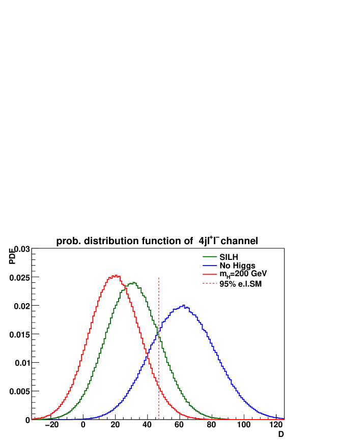
The normalized frequency of the discriminant for the three scenarios is reported in Fig. 14 for . The red curve refers to a Higgs of 200 GeV while the green one refers to the SILH model and the blue one to the no–Higgs case. The dotted vertical line in the plot marks the 95% exclusion limit for the SM predictions.
The channel, as expected, is the one with the best discriminating power between the BSM models and the SM. The expected number of events in this final state is about ten times larger than in the channel.
The probability of an experiment to find a result incompatible with the SM at 95%CL assuming that the Higgsless model is realized in Nature is of the order of 96% for and decreases to about 84% for . For the SILH model the PBSM@95%CL varies between 35% and 17%.
8 Combining all channels
In this section we derive the probability that, assuming that either the Higgsless scenario or the instance of SILH model we have considered is realized in Nature, the results of the measurements of the , and channels at the LHC yield results which are outside the 95% probability region for the SM. In order to do so, it is convenient to rephrase the method employed in Ref. [30] and in the previous sections for the case of a single measurement. In the new language the generalization to a set of several simultaneous measurements will be obvious. Given two models and and the probability distributions of some physical observable , and , the 95%CL region for model can be defined considering the probability ratio
| (5) |
One can consider all the possible values with and fix with the condition that
| (6) |
For distributions like those in Fig. 10, 13 and 14 this procedure would lead for the SM to the one–sided exclusion regions shown by a vertical dotted line. The probability for model to yield a result outside this 95%CL region for would then be
| (7) |
Eqs.(5–7) can be easily generalized to a set of observables introducing the joint probability and transforming the integrals Eqs.(6–7) to –dimensional ones. In the present case we have assumed the probabilities to be independent and defined
| (8) |
This method is obviously equivalent to the one, based on the Neyman–Pearson lemma, of using the likelihood ratio for discriminating between two different hypotheses for a multidimensional test statistics [39].
In Tab. 10 we present the PBSM@95%CL for the Higgsless and SILH model compared to the SM predictions for each channel and for their combination for . We assume and sum over all electron and muon channels.
| channel | NOH | SILH |
|---|---|---|
| 80.0% | 19.5% | |
| 77.1% | 16.8% | |
| 96.5% | 35.9% | |
| semi-leptonic | 99.4% | 41.2% |
| all | 99.9% | 51.5% |
Tab. 10 shows, within the limits of the parton level, lowest-order analysis presented in this paper, that if no Higgs is present we are essentially certain that the LHC will obtain combined results in the , and channels which will lay outside the 95% CL region of the Standard Model. If however some version of the SILH models discussed in Ref. [19] is instead realized the probability of such an outcome drops to about 50%.
| channel | NOH | SILH | ||||
|---|---|---|---|---|---|---|
| 80.0% | 80.0% | 80.0% | 19.5% | 19.5% | 19.5% | |
| 90.1% | 77.1% | 38.5% | 22.5% | 16.8% | 8.5% | |
| 99.9% | 96.5% | 79.9% | 51.8% | 35.9% | 25.1% | |
| semi-leptonic | 99.99% | 99.4% | 90.1% | 58.9% | 41.2% | 26.8% |
| all | 99.999% | 99.9% | 98.7% | 66.4% | 51.5% | 39.8% |
In Tab. 11 we show how our results depend on the size of the separation cut among jets, comparing our standard choice with the the requirement of a stronger separation, and with case in which no cone separation among jet is required, . In all cases each jet pair is required to have an invariant mass of at least 60 GeV. As already mentioned in Sect. 4, at large transverse momentum, jet pairs with mass comparable to the mass of electroweak bosons can merge into one single jet when an angular measure like is adopted for reconstructing jets. Since we insist on requiring four jets in the final state these events are discarded and the cross sections are smaller at larger . However since the ’s transverse momentum distribution is harder in the SILH model and in the Higgsless case than in the SM the PBSM@95%CL decreases significantly at larger values of for the semileptonic channels. The overall combination is less sensitive since the channel is not affected by the cut.
In several analyses [42] it has been shown that significantly better results in the identification of hadronic decays of vector boson, Higgs bosons or supersymmetric partners of ordinary particles can be obtained analyzing the substructure of high– jets in order to separate ordinary QCD jets from those generated by the decay of heavy objects. Such an approach might overcome the loss in discrimination between the SM and the BSM scenarios at large . We leave this possibility for further work.
9 Conclusions
We have examined at parton level the processes , and including all irreducible backgrounds contributing to these six parton final states. We have considered three scenarios: a light Higgs SM framework with , one instance of the SILH models and an infinite mass Higgs scenario in order to determine whether the two BSM models can be distinguished from the SM at the LHC using boson–boson scattering. For the semileptonic channels, the largest background is at which can be subtracted looking at the distribution of the invariant mass of the two most central jets in the region outside the weak boson mass window. We have estimated the probability, in the two BSM scenarios, of finding, combining all set of measurements, a result outside the 95% probability range in the Standard Model. This probability turns out to be about 99.9% for the Higgsless case and 51.5% for the SILH model. These probabilities correspond to an integrated luminosity of and to the sum of all electron and muon channels for a mass of the reconstructed pair of vector bosons larger than 600 GeV. Jet resolution plays a crucial role in the present analysis as in all processes in which high transverse momentum vector bosons or top particles are present and decay hadronically.
Acknowledgments
A.B. wishes to thank the Dep. of Theoretical Physics of Torino University
for support.
We gratefully acknowledge discussions with R. Rattazzi on the
details of the SILH model.
This work has been supported by MIUR under contract 2006020509 004 and by the
European Community’s Marie-Curie Research Training Network under contract
MRTN–CT–2006–035505 Tools and Precision Calculations for Physics Discoveries
at Colliders
References
- [1] The LEP Collaborations (ALEPH, DELPHI, L3 and OPAL), the LEP Electroweak Working Group and the SLD Heavy Flavour Group, A combination of preliminary Electroweak measurements and constraints on the Standard Model, LEPEWWG/2007-01; http://lepewwg.web.cern.ch/LEPEWWG.
- [2] The LEP Collaborations (ALEPH, DELPHI, L3 and OPAL), the LEP Electroweak Working Group and the SLD Heavy Flavour Group, http://lepewwg.web.cern.ch/LEPEWWG.
- [3] CDF Collaboration and D0 Collaboration, To appear in the proceedings of 44th Rencontres de Moriond on QCD and High Energy Interactions, La Thuile, Valle d’Aosta, Italy, 14-21 Mar 2009, arXiv:0905.2090 [hep-ex]; CDF Collaboration and D0 Collaboration, To appear in the proceedings of 44th Rencontres de Moriond EW 2009: Electroweak Interactions and Unified Theories, La Thuile, Italy, 7-14 Mar 2009, arXiv:0906.1403 [hep-ex]
- [4] Proceedings of the Large Hadron Collider Workshop, Aachen 1990, CERN Report 90–10, G. Jarlskog and D. Rein (eds.).
- [5] A. Djouadi, The Anatomy of Electro–Weak Symmetry Breaking. Tome I: The Higgs in the Standard Model, [arXiv:hep-ph/0503172].
- [6] ATLAS Collaboration, Detector and Physics Performance Technical Design Report, Vols. 1 and 2, CERN–LHCC–99–14 and CERN–LHCC–99–15.
- [7] K.A. Assamagan, M. Narain, A. Nikitenko, M. Spira, D. Zeppenfeld (conv.) et al., Report of the Higgs Working Group, Proceedings of the Les Houches Workshop on “Physics at TeV Colliders”, 2003, [arXiv:hep-ph/0406152].
- [8] CMS Collaboration,Technical Design Report, Vols. 1 and 2, CERN/LHCC 2006–001 and CERN/LHCC 2006–021.
- [9] M.S. Chanowitz, Strong WW scattering at the end of the 90’s: theory and experimental prospects. In Zuoz 1998, Hidden symmetries and Higgs phenomena 81-109. [arXiv:hep-ph/9812215]
- [10] D. B. Kaplan and H. Georgi, Phys. Lett. B 136 (1984) 183.
- [11] N. Arkani-Hamed, A. G. Cohen and H. Georgi, Phys. Lett. B 513 (2001) 232.
- [12] N. Arkani-Hamed, A. G. Cohen, E. Katz and A.E. Nelson, JHEP 0207, 034 (2002), [arXiv:hep-ph/0206021].
- [13] N. S. Manton, Nucl. Phys. B 158 (1979) 141; Y. Hosotani, Annals Phys. 190 (1989) 233.
- [14] C. Csaki, C. Grojean and H. Murayama, Phys. Rev. D 67 (2003) 085012; C. A. Scrucca, M. Serone and L. Silvestrini, Nucl. Phys. B 669 (2003) 128.
- [15] K. Agashe, R. Contino and A. Pomarol, Nucl. Phys. B 719 (2005) 165.
- [16] S. Chang, JHEP 0312, 057 (2003), [arXiv:hep-ph/0306034].
- [17] G.F. Giudice, J.Phys.Conf.Ser.110:012014,2008, arXiv:0710.3294 [hep-ph].
- [18] R. Contino, T. Kramer, M. Son and R. Sundrum, JHEP 0705 (2007) 074.
- [19] G.F. Giudice, C. Grojean, A. Pomarol, R. Rattazzi, JHEP 0706:045,2007, [arXiv:hep-ph/0703164].
- [20] R. Barbieri, B. Bellazzini, V.S. Rychkov, A. Varagnolo, Phys.Rev.D76:115008,2007, arXiv:0706.0432 [hep-ph].
- [21] T. Appelquist and C.W. Bernard, Phys. Rev. D22 (1980) 200; A.C. Longhitano, Phys. Rev. D22 (1980) 1166; A.C. Longhitano, Nucl. Phys. B188 (1981) 118;T. Appelquist and G.H. Wu, Phys. Rev. D48 (1993) 3235(1993) [hep-ph/9304240].
- [22] M.J. Duncan, G.L. Kane and W.W. Repko, Nucl. Phys. B272 (1986) 517; D.A. Dicus and R. Vega, Phys. Rev. Lett. 57 (1986) 1110; J.F. Gunion, J. Kalinowski and A. Tofighi–Niaki, Phys. Rev. Lett. 57 (1986) 2351.
- [23] R.N. Cahn, S.D. Ellis, R. Kleiss and W.J. Stirling, Phys. Rev. D35 (1987) 1626; V. Barger, T. Han and R. Phillips, Phys. Rev. D37 (1988) 2005 and D36 (1987) 295; R. Kleiss and J. Stirling, Phys. Lett. 200B (1988) 193; V. Barger et al., Phys. Rev. D42 (1990) 3052; V. Barger et al., Phys. Rev. D44 (1991) 1426; V. Barger et al., Phys. Rev. D46 (1992) 2028; D. Froideveaux, in Ref. [4] Vol II, p. 444; M. H. Seymour, in Ref. [4] Vol II, p. 557; U. Baur and E.W.N. Glover, Phys. Lett. B252 (1990) 683; D. Dicus, J. Gunion and R. Vega, Phys. Lett. B258 (1991) 475; D. Dicus, J. Gunion, L. Orr and R. Vega, Nucl. Phys. B377 (1991) 31; J. Bagger et al.,Phys. Rev. D49 (1994) 1246;V. Barger, R. Phillips and D. Zeppenfeld, Phys. Lett. B346 (1995) 106; J. Bagger et al.,Phys. Rev. D52 (1995) 3878;K. Iordanidis and D. Zeppenfeld, Phys. Rev. D57 (1998) 3072; R. Rainwater and D. Zeppenfeld, Phys. Rev. D60 (1999) 113004; erratum ibid D61 (2000) 099901.
- [24] E. Accomando, A. Ballestrero, S. Bolognesi, E. Maina and C. Mariotti, JHEP 0603 (2006) 093 [arXiv:hep-ph/0512219].
- [25] E. Accomando, A. Ballestrero, A. Belhouari and E. Maina, Phys. Rev. D 75 (2007) 113006 [arXiv:hep-ph/0603167].
- [26] G. Bevilacqua, in F. Ambroglini et al., Proceedings of the Workshop on Monte Carlo’s, Physics and Simulations at the LHC PART II, Frascati, Italy.
- [27] K. Cheung, C. Chiang and T. Yuan, Phys. Rev.D78(2008)051701, arXiv:0803.2661 [hep-ph].
- [28] B. Jäger, C. Oleari and D. Zeppenfeld, JHEP 0607 (2006) 015,[hep-ph/0603177]; B. Jäger, C. Oleari and D. Zeppenfeld, Phys.Rev.D73:113006,2006, [hep-ph/0604200]; G. Bozzi, B. Jäger, C. Oleari and D. Zeppenfeld, Phys.Rev.D75:073004,2007 , [hep-ph/0701105].
- [29] K. Arnold et al., arXiv:0811.4559 [hep-ph].
- [30] A. Ballestrero, G. Bevilacqua, and E. Maina JHEP 05 (2009) 015, [arXiv:0812.5084].
- [31] R. Barate et al. [LEP Working Group for Higgs boson searches and ALEPH, DELPHI, L3 and OPAL Collaborations], Phys. Lett. B 565 (2003) 61 [arXiv:hep-ex/0306033].
- [32] A. Ballestrero, A. Belhouari, G. Bevilacqua, V. Kashkan and E. Maina, Comp. Phys. Commun. 180 (2009) 401, arXiv:0801.3359 [hep-ph].
- [33] E. Accomando, A. Ballestrero, E. Maina, JHEP 0507 (2005) 016, [arXiv:hep-ph/0504009].
- [34] A. Ballestrero and E. Maina, Phys. Lett. B350 (1995) 225, [arXiv:hep-ph/9403244].
- [35] A. Ballestrero, PHACT 1.0 - Program for Helicity Amplitudes Calculations with Tau matrices’ [arXiv:hep-ph/9911318] in Proceedings of the 14th International Workshop on High Energy Physics and Quantum Field Theory (QFTHEP 99), B.B. Levchenko and V.I. Savrin eds. (SINP MSU Moscow), pg. 303.
-
[36]
F. Maltoni, T. Stelzer, JHEP 0302 (2003) 027;
T. Stelzer and W. F. Long, Comput. Phys. Commun. 81 (1994) 357;
J. Alwall et al., JHEP 0709:028,2007, arXiv:0706.2334;
H. Murayama, I. Watanabe and K. Hagiwara, KEK-91-11. - [37] J. Alwall et al., A Standard format for Les Houches event files. Written within the framework of the MC4LHC-06 workshop: Monte Carlos for the LHC: A Workshop on the Tools for LHC Event Simulation (MC4LHC), Geneva, Switzerland, 17-16 Jul 2005, Comp. Phys. Commun. 176 (2007) 300, [arXiv:hep-ph/0609017].
- [38] CTEQ Coll.(H.L. Lai et al.) Eur. Phys. J. C12 (2000) 375.
- [39] G. Cowan, Statistical Data Analysis, Oxford University Press, 1998.
- [40] A.D. Martin, R.G. Roberts, W.J. Stirling and R.S. Thorne, Eur. Phys. J. C28 (2003) 455, [hep-ph/0211080].
- [41] A.D. Martin, R.G. Roberts, W.J. Stirling and R.S. Thorne, Eur. Phys. J. C35 (2004) 325, [hep-ph/0308087].
-
[42]
J.M. Butterworth,B.E. Cox and J.R. Forshaw, Phys. Rev. D65 (2002) 96014,
[arXiv:hep-ph/0201098];
J.M. Butterworth, J. Ellis and A.R. Raklev, JHEP 0705 (2007) 033, [arXiv:hep-ph/0702150];
J.M. Butterworth,A. Davison, M. Rubin and G. Salam, Phys. Rev. Lett. 100(2008)242001, arXiv0802.2470 [hep-ph].