The Gas Consumption History to Redshift 4

Abstract

Using the observations of the star formation rate and H I densities to $z\sim 4$, with measurements of the Molecular Gas Depletion Rate (MGDR) and local density of H₂ at $z=0$, we derive the history of the gas consumption by star formation to $z\sim 4$. We find that closed-box models in which H₂ is not replenished by H I require improbably large increases in $\rho(H_{2})$ and a decrease in the MGDR with lookback time that is inconsistent with observations. Allowing the H₂ used in star formation to be replenished by H I does not alleviate the problem because observations show that there is very little evolution of $\rho_{HI}(z)$ from $z=0$ to $z=4$. We show that to be consistent with observational constraints, star formation on cosmic timescales must be fueled by intergalactic ionized gas, which may come from either accretion of gas through cold (but ionized) flows, or from ionized gas associated with accretion of dark matter halos. We constrain the rate at which the extraglactic ionized gas must be converted into H I and ultimately into H₂. The ionized gas inflow rate roughly traces the SFRD: about 1 – 2 $\times 10^{8}$ M_☉ Gyr^-1 Mpc^-3 from $z\simeq 1-4$, decreasing by about an order of magnitude from $z=1$ to $z=0$ with details depending largely on MGDR(t). All models considered require the volume averaged density of $\rho_{H_{2}}$ to increase by a factor of 1.5 – 10 to $z\sim 1.5$ over the currently measured value. Because the molecular gas must reside in galaxies, it implies that galaxies at high $z$ must, on average, be more molecule rich than they are at the present epoch, which is consistent with observations. These quantitative results, derived solely from observations, agree well with cosmological simulations.

1. Introduction

The time variation of the mean star formation rate in galaxies is by now well established (Madau et al., 1996; Steidel et al., 1999; Hippelein et al., 2003; Hopkins & Beacom, 2006). The star formation rate is either flat or slowly rising with time, reaching a maximum near $z\sim$ 1 – 2, and then declines precipitously down to the current epoch. This change in the star formation rate must be closely coupled to both the inventory of gas available for star formation, and the way in which this gas is channeled into galaxies.

Stars condense only from molecular gas at the current epoch and at all epochs in the past. This statement derives from both observational and theoretical considerations. Observationally, the youngest stars are always found to be associated with their nascent molecular material both in the local Universe and at high $z$ (e.g. Blaauw 1964; Herbig & Kameswara Rao 1972; Schwartz et al. 1973; Omont et al. 1996; Carilli et al. 2002). The interstellar gas in star forming regions is almost completely molecular, representing a stable phase of the ISM with little atomic content (Burton et al., 1978). Theoretically, there is general consensus that the initiation of star formation requires the nascent gas to become Jeans unstable, probably mediated by magnetic fields (Shu et al., 1987). In star forming regions, $T$ is typically 10 - 20 K, but in any event cannot be less than 2.7 K. In order to get a solar mass star at 10 K, the Jeans instabiliy criterion would require a density of $\rho_{J}>(kT/{\mu}{m_{H}}G)^{3}(\pi^{5}/36M_{J}^{2})\sim 10^{6}{\rm cm}^{-3}$ if a molecular core forms a star at 100% efficiency. The density must be higher if the efficiency is lower as many observations now suggest (e.g. Motte et al. 1998; Alves et al. 2007; Myers 2008). In order to reach these temperatures and densities, the gas must be fully molecular in order to achieve the necessary cooling. We would therefore expect that, in a broad sense, the gas consumption rate is closely tied to the star formation rate.

Unfortunately, there are few constraints on the gas from observations because little is known about the distribution of neutral gas at high $z$. There are very few detections of atomic gas in emission at $z\gtrsim$ 0.1, and what little we know about the atomic gas comes from Lyman-alpha lines seen in absorption toward quasars and radio-loud AGN (e.g. Prochaska & Wolfe 2009; Wolfe et al. 2005; Zwaan & Prochaska 2006). Molecular line observations at high-$z$ have been largely limited to the brightest objects, though some recent observations at $z\sim 2$ have begun to probe lower luminosity systems (Förster Schreiber et al., 2009; Daddi et al., 2009; Tacconi et al., 2010).

Gas consumption by star formation in galaxies has been investigated previously via observations of the gas depletion time, $\tau_{dep}=M_{gas}/SFR$. This represents the amount of time it will take the galaxy to completely exhaust its gas supply at the current star formation rate. Studies of individual local disk galaxies find depletion times on the order of a few Gyr, much shorter than the Hubble time (e.g. Larson et al. 1980; Kennicutt et al. 1994). This is the gas depletion problem: without some form of gas replenishment, star formation in disk galaxies should be coming to an abrupt end. One proposed solution is stellar recycling, which Kennicutt et al. (1994) find can extend the gas depletion times in many local disk galaxies by a factor of 1.5 to 4. Gas accretion has long been suggested as a solution to the gas depletion problem as well, and observational support for inflow is accumulating. Sancisi et al. (2008) review the observational evidence for gas accretion such as galaxy interactions and minor mergers, high velocity clouds (HVCs), extra-planar gas and warped or lop-sided HI disks. These observations yield an estimate for the ’visible’ gas accretion rate onto a typical disk galaxy of $\sim 0.2$ M_⊙ yr^-1, which falls short of the typical star formation rate of $\sim 1$ M_⊙ yr^-1. These studies focus on recycling and inflow in local disk galaxies, but one may ask how does gas consumption evolve with redshift?

The time evolution of gas in disk galaxies has been studied on large scales using observations of damped Ly$\alpha$ systems (DLAs) to infer the cosmic mass density of HI as a function of redshift. The cosmic mass density is the mass density averaged over a large volume so as to be representative of a typical Mpc^-3 of the universe. Lanzetta et al. (1995) and Pei & Fall (1995) build simple models of gas consumption focusing on the chemical evolution of the gas using the cosmic mass density of HI and observed metallicities as inputs. Their models predict the star formation rate density (SFRD) of the universe as a function of redshift for their chosen inflow and outflow parameters. However, the SFRD is now becoming increasingly well constrained by observations and we can use SFRD$(z)$ as an input to our models in order to place constraints on the gas inflow rates.

Finally, this problem has been approached using numerical simulations to explain observations of the SFRD and galaxy properties. The shape of the SFRD has been investigated using cosmological, hydrodynamical simulations that include prescriptions for star formation and feedback (e.g. Hernquist & Springel 2003; Schaye et al. 2010). These studies suggest that the shape of the SFRD at high redshifts is determined by the buildup of dark matter halos and the gas brought in with them, and the decline of the SFRD at low redshifts is due to lower cooling rates in the halo gas, gas exhaustion and stellar and black hole feedback. The results of simulations have also been used to build simple models in order to better understand gas accretion to fuel star formation in galaxies. Bouché et al. (2009) build a simple model of gas consumption starting with simulated halo growth histories with different prescriptions for gas accretion and star formation. The predictions from the different prescriptions are compared to the observed SFR-Mass and Tully-Fisher relations for galaxies from $z\sim 2$ to $z=0$. The authors find that the prescription for gas accretion modeled on cold flows with halo mass cutoffs agrees best with observations.

In this paper, we look at the issue in reverse. We build simple models of gas consumption based solely on observations in order to understand the roles of the different phases of gas in star formation in galaxies. Using observations at $z$ = 0, we examine which quantitative conclusions can be extrapolated to high $z$, and using observations of the star formation history, we make several inferences about how the gas consumption into stars must have proceeded. We find that the relationship of the inventory of gas to that of the stars is not straightforward: the observations imply that that all phases of the interstellar and intergalactic medium must be taken into account in order to understand how the gas forms stars. Building a model that includes all the gas phases, we make predictions about gas densities and their variation at intermediate- and high-$z$, and how this gas must have been accreted into galaxies.

The paper is organized as follows. §2 describes the observations of the SFRD, MGDR, $\rho_{H_{2}}$ and $\rho_{HI}\$that we use as inputs to our models. In §3, we build three models to fit the observations: the restricted closed box model, the general closed box model and the open box model. In §4, we discuss potential changes to our star formation prescription at high redshift and examine the predictions of the open box model. Throughout this paper, we adopt a standard $\Lambda$CDM cosmology with (h, $\Omega_{M}$, $\Omega_{\Lambda}$) = (0.7, 0.3, 0.7). All of the densities are in comoving units.

2. Observations

2.1. SFRD

The observed (comoving) star formation rate density, SFRD, was estimated by Madau et al. (1996) over a large range of $z$ and re-examined by several other investigators (Steidel et al., 1999; Hippelein et al., 2003; Hopkins & Beacom, 2006). We will focus on the results of Hopkins & Beacom (2006), a compilation of SFRD measurements at different wavelengths. The measurements are converted to a common cosmology, SFRD calibration, and dust obscuration correction; the data are then fit to a piecewise linear form in $\log(1+z)$ vs. $\log(SFRD)$ space as well as the parameterization from Cole et al. (2001). Hopkins & Beacom (2006) find that changing the assumed IMF corresponds to a simple change in the overall amplitude of the SFRD, so each fit is done using two extreme IMF forms in order to provide bounds on the actual form. These two extreme forms for the IMF are a modified Salpeter A IMF and the form of Baldry & Glazebrook (2003). Fig. 1 plots the fits for the two IMFs in red and blue. We have smoothed the original piecewise linear fits from Hopkins & Beacom (2006) for our models (solid lines). The form of the smoothed piecewise linear fit is given in Appendix A.

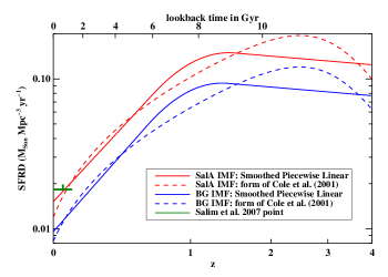
Figure 1.— Comparison of forms of the SFRD. The solid curves show our smoothed version of the piecewise linear fits from Hopkins & Beacom (2006); the dashed curves show the fits to the Cole et al. (2001) form. Two IMFs are plotted: the modified Salpeter A IMF (SalA IMF; red) and the IMF from Baldry & Glazebrook (2003) (BG IMF; blue). The green symbol denotes the SFRD at $z=0$ measured by Salim et al. (2007).

At $z$ = 0, the SFRD fits from Hopkins & Beacom (2006) predict a local SFRD of $(0.8-1.5)\times 10^{-2}$ M${}_{\sun}\,{\rm Mpc^{-3}}$ yr^-1. In an extensive study of galaxies in the local universe (to $z$ = 0.1), Salim et al. (2007) find that the SFRD is $1.828^{+0.148}_{-0.039}\times 10^{-2}\ h_{70}$ M${}_{\sun}\,{\rm Mpc^{-3}}$ yr^-1 from UV observations (using the Chabrier 2003 IMF), a value they argue is the most accurate determination of this number to date. This value (shown as a data point in Fig. 1) is indeed close to those found from other recent investigations (Houck et al., 2007; Hanish et al., 2006) and is also in reasonable agreement with the forms of Hopkins & Beacom (2006).

The agreement between the locally determined SFRD and extrapolation from studies at higher $z$ (Hopkins & Beacom, 2006; Steidel et al., 1999; Hippelein et al., 2003) is encouraging and provides some confidence that the star formation rates and their time variation are being measured reliably. While somewhat different functional forms for the decline of the SFRD with time have been proposed in the literature, e.g., log(SFRD) has been found to be linear in $z$ (Steidel et al., 1999), in $t$ (Hippelein et al., 2003), and in $\log(1+z)$ (Hopkins & Beacom, 2006), these differences have only a small quantitative effect in what follows.

2.2. MGDR

2.2.1 Measurements at z = 0

The star formation efficiency, SFE, is often defined as the star formation rate per comoving volume divided by the mass per comoving volume of gas; its units are yr^-1 (Leroy et al. 2008 and references therein). Defined in this way, the SFE is not properly an efficiency, but a rate, and we drop this unfortunate usage even though it has become firmly entrenched in the observational literature. Since we are interested in SFE_M, the star formation rate density divided by the density of molecular gas, $\rho_{H_{2}}$, we introduce the molecular gas depletion rate, MGDR, to replace the usage of SFE_M. We define MGDR as SFRD divided by the density of molecular hydrogen, $\rho_{H_{2}}$ (this does not include He). The inverse of MGDR is the molecular gas depletion time, $\tau_{\mathrm{M}}$, which represents the time it takes to consume all of the molecular gas at the current rate of star formation.

Recently, Leroy et al. (2008) have measured MGDR($z$ = 0) from a comprehensive analysis of 23 nearby galaxies. The results are based on H I surface densities measured from the THINGS H I survey (Walter et al., 2008), H₂ surface densities inferred from the BIMA SONG (Helfer et al., 2003) and HERACLES (Leroy et al. 2008b) CO surveys, and star formation rates from both SINGS (Kennicutt et al., 2003) and GALEX (Gil de Paz et al., 2007) data. The galaxies surveyed include spiral and dwarf galaxies and the analysis was done on a pixel-by-pixel basis convolved to a common resolution, typically $\sim$800 pc. This comparison is the most extensive work done to date and the authors find a remarkable constancy of MGDR over a wide range of conditions: $0.525\pm 0.25{\rm\ Gyr}^{-1}$, equivalent to a molecular gas depletion time of 1.9 Gyr. Their measured star formation rates and H₂ column densities vary by three orders of magnitude averaged over entire galaxies, and the pixel-by-pixel values vary even more. Thus the constancy of the MGDR occurs over a wide range of conditions both within galaxies (including nuclei and disks) and from galaxy to galaxy.

2.2.2 Measurements at high z

The Leroy et al. (2008) study only applies to galaxies near $z=0$. To extend the range of $z$ we appeal to observations of the MGDR in normal, $z\gtrsim 1$ galaxies. Daddi et al. (2009) report the SFR and total gas mass for six, near-infrared selected BzK galaxies at $z\sim 1.5$. Using numerical simulations, they calculate a conversion factor $\alpha_{CO}=M_{gas}/L_{CO}=3.6\pm 0.8$ M_⊙ (K km s^-1 pc²)^-1. This value is close to a Milky Way-like value of $\alpha_{CO}\sim 4.6$ and excludes a typical ULIRG value of $\alpha_{CO}\sim 1$. This gas mass includes He, so we divide by $1.4$ to calculate the MGDR, which we have defined to not include He. The MGDR values for these six galaxies in Daddi et al. (2009) vary between 1.9 and 4.7 Gyr^-1, three to nine times the Leroy et al. (2008) value for $z=0$. Apparently, molecular gas is consumed by star formation at a much higher rate at high redshift than it is today.

Similarly, Tacconi et al. (2010) have made an extensive survey of normal, star forming galaxies at redshifts 1 and 2, measuring the MGDR for a sample of 19 galaxies. At each redshift locus, the selected galaxies sample the high mass end of the main sequence galaxy population in the M_∗-SFR plane. The Tacconi et al. (2010) results use a Milky Way-like value for $\alpha_{CO}$. They find MGDR values in agreement with the Daddi et al. (2009) values at $z\sim 1.5$. The data points from these studies are plotted in Figures 3 and 5: Daddi et al. (2009) as purple diamonds and Tacconi et al. (2010) as green squares.

In samples of galaxies selected by different optical and near-IR criteria, Reddy et al. (2005) find that BzK, BX/BM and DRG selected galaxies account for an SFRD of $\sim 0.1$ M${}_{\sun}\,{\rm Mpc^{-3}}$ yr^-1 in the range $1.4<z<2.6$. This is most of the observed SFRD (see Fig. 1). More recently, Reddy et al. (2008) find that galaxies with $L_{\mathrm{IR}\,}\approx L_{\mathrm{bol}\,}\lesssim 10^{12}\ L_{\odot}$ account for $\approx 70\%$ of the SFRD at $1.9\leq z<2.7$. The BX/BM, BzK and DRG selection criteria sample luminous, star forming galaxies with L $\sim 10^{11}-10^{12}$ L_⊙ and SFR $\sim 10-500$ M_☉ yr^-1 (Tacconi et al., 2008). Therefore, these systems sampled by Daddi et al. (2009) and Tacconi et al. (2010) account for most of the SFRD at these redshifts so that the MGDR value that typifies these galaxies should describe the average cosmic MGDR in Eq. 1. This motivates us to use these samples to constrain our guessed forms of the MGDR at other redshifts.

Numerous other authors have estimated the MGDR from individual high redshift galaxies, or from starbursts or ULIRGS (e.g. Gao & Solomon 2004), and all have found that the MGDR is greater in these galaxies than is typical of galaxies at $z$ = 0. In fact, there is no observational evidence for a declining MGDR with increasing redshift to at least $z\sim 4$. Taken together, all of these observations lead us to reject any model of gas consumption that requires lower MGDR values at redshifts significantly greater than zero.

2.3. $\rho_{H_{2}}$

Using a combination of CO and H I measurements in the local universe, Obreschkow & Rawlings (2009) have determined the density of H₂ at $z=0$, $\rho_{H_{2}}(0)$, to be 1.9 – 2.8 $\times 10^{7}$ h M${}_{\sun}\,{\rm Mpc^{-3}}$. The range of values corresponds to different assumptions about how metallicity affects the CO-to-H₂ conversion ratio (the authors quote an error of $\pm 40\%$ on each individual calculated value). Using $h=0.7$ gives $\rho_{H_{2}}(0)=(1.3-2.0)\times 10^{7}$ M${}_{\sun}\,{\rm Mpc^{-3}}$, or an average value of $1.65\times 10^{7}$ M${}_{\sun}\,{\rm Mpc^{-3}}$. This value is within 50% of the estimate of $\rho_{H_{2}}(0)=1.1\times 10^{7}$ M${}_{\sun}\,{\rm Mpc^{-3}}$ by Zwaan & Prochaska (2006) (no error quoted) using a different set of observations and should therefore be reasonably reliable.

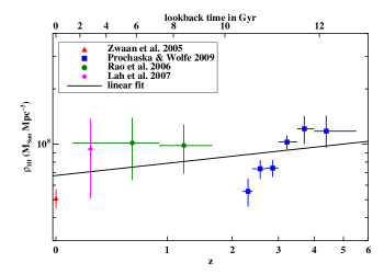
Figure 2.— Data points for the comoving $\rho_{HI}\$from Zwaan et al. (2005); Rao et al. (2006); Lah et al. (2007); and Prochaska & Wolfe (2009) with linear fit in $\log(1+z)$ vs $\log(\rho_{HI})$ space.

2.4. $\rho_{HI}\$

A number of recent studies have reported measurements of the mean H I comoving mass density in galaxies, $\rho_{HI}(z)$, from the local universe to $z\sim 6$. At $z=0$, Zwaan et al. (2005) present a study of the H I mass function using the H I Parkes All Sky Survey (HIPASS) data. At low redshift, Lah et al. (2007) calculate $\rho_{HI}\$by co-adding H I 21-cm emission from galaxies with known positions and redshifts. At higher redshifts, estimates of $\rho_{HI}\$are mainly obtained from DLA studies (Rao et al., 2006; Prochaska & Wolfe, 2009). We use these observations of H I to construct an analytical form for $\rho_{HI}\$as a function of $z$. We fit a straight line to these points in $\log(1+z)$ vs $\log(\rho_{HI})$ space. The data points and the fit are shown in Fig. 2. The observations suggest very little evolution of $\rho_{HI}\$, which increases by only a factor of 2-3 between $z=0$ and $z=6$. A more recent DLA study (Noterdaeme et al., 2009) using SDSS DR7 finds the values at $z\sim 2$ to 3 to be somewhat higher than the Prochaska & Wolfe (2009) points; this would make our linear fit in Fig. 2 correspond even better to the observations.

3. Building a Model to Fit the Observations

The observations above allow us to compare the evolution of the SFRD and $d\rho_{H_{2}}/dt$. We start with the simplest model possible: a closed box of H₂ being turned into stars at the rate of $d\rho_{H_{2}}/dt$. In this closed box model, we initially assume that the MGDR is constant in time (the restricted closed box model; §3.1) and subsequently relax this condition (the general closed box model; §3.2). The failure of both models motivates us to consider an open box model (§3.3), where we allow the densities of all four phases of the IGM – stars, H₂, H I  and H II – to vary to match the observational constraints.

We assume that the molecular gas is depleted only through star formation, and that any $\mathrm{H_{2}}$ dissociated or ionized by star formation is instantaneously returned to the molecular state. Given the short timescales for the formation of molecular gas from its atomic form, $\sim 10^{6}$ yr at the relevant densities (Hollenbach & Salpeter, 1971; Cazaux & Tielens, 2004), this approximation should be a good one for the purposes of this paper. In any event, if we define $d\rho_{H_{2}}/dt$ to be the net flow rate of molecular gas into stars, then there is no ambiguity.

We write the statement that star formation occurs only through the depletion of molecular gas:

$$SFRD=MGDR\times\rho_{H_{2}}\,.$$ (1)

This equation was used to infer the individual MGDR for a sample of nearby galaxies with a wide of range of SFRs and $H_{2}$ column densities, where it was found that $MGDR\approx 0.5$ Gyr^-1 to a remarkable constancy (Leroy et al. 2008, see §2.2). We use this prescription for the SFRD for our models but we note that the form may change at higher redshift (See §4.1).

It is also interesting to note that if we divide the observed global star formation rate density SFRD$(z=0)\sim$ (0.8 – 1.8) $\times 10^{-2}M_{\sun}\,{\rm Mpc^{-3}}$ yr^-1 (Hopkins & Beacom, 2006; Salim et al., 2007) by the observed $\rho_{H_{2}}(0)=(1.3-2.0)\times 10^{7}M_{\sun}\,{\rm Mpc^{-3}}$ (Obreschkow & Rawlings, 2009), we obtain a range of MGDR that is consistent with the values of Leroy et al. (2008). Given that stars must form from molecular gas, this result is not surprising. Nevertheless, the agreement is reassuring because it is based on different data sets and different methods of determining the relevant quantities. It also suggests, combined with the arguments in §1 that Eq. 1 can be extrapolated to all $z$.

We use mass densities instead of mass surface densities, which are used by observers, but note that these are roughly equivalent because for the most part, the stars, H I and H₂ are generally confined to thin disks within galaxies.

3.1. The Restricted Closed Box Model

In the closed box model, we consider only stars and H₂, and allow $\rho_{H_{2}}$ to be converted into stars at the star formation rate density, SFRD:

$$\frac{d\rho_{H_{2}}}{dt}=-SFRD\,.$$ (2)

For the moment, we consider a restricted closed box model in which we take the MGDR to be constant as a function of redshift. To assess the ability of this model to fit observations, we first combine eqs. (1) and (2) to obtain $d(SFRD)/dt=MGDR\times SFRD$. We then note that our piecewise linear fit to the observed SFRD as a function of time (Appendix A) implies $d(SFRD)/dt\sim(.24\,{\rm Gyr}^{-1})\times SFRD$, where the coefficient is about half of the observed MGDR (Leroy et al., 2008).

In other words, from the assumption of a constant MGDR at the present epoch in a closed box H₂ model, we find that the star formation rate is declining only half as fast as expected given our current reservoir of molecular gas. It is this discrepancy in the derivatives of the observed cosmic star formation rate and the rate at which we observe molecular gas being converted into stars that we call the cosmic molecular gas depletion problem. We note here that given the uncertainties in the observations, this factor of two in itself is not a strong argument against the closed box model, but we will show in general that observational constraints rule out any closed box model.

3.2. The General Closed Box Model

We now relax the assumption of a constant MGDR in the closed box model in §3.1. To study the predictions of this model, we calculate $\rho_{H_{2}}(z)$ by integrating Eq. (2) and using the observed SFRD$(z)$ as an input. We then divide SFRD$(z)$ by $\rho_{H_{2}}(z)$ to obtain MGDR$(z)$. The results are shown in Fig. 3, where $\rho_{H_{2}}(0)$ is set to the mean value from Obreschkow & Rawlings (2009). The uncertainties in the SFRD (due to the IMF) discussed in §2.1 are seen to have only a minor effect on the resulting $\rho_{H_{2}}(z)$ and MGDR$(z)$.

Fig. 3 shows that $\rho_{H_{2}}(t)$ increases by a factor of $\sim 10$ from $z=0$ to 1, and MGDR decreases with increasing redshift, contrary to the observational results discussed in §2.2. Thus, even the general closed box model is at odds with the observations, leading us to our next model.

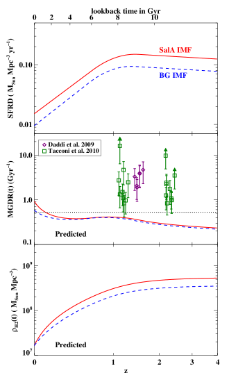
Figure 3.— The predicted MGDR(t) and $\rho_{H_{2}}(t)$ in the closed box model. The top panel shows the input SFRD forms (the smoothed piecewise linear fits from Fig. 1). The middle and bottom panels show the MGDR and $\rho_{H_{2}}(t)$, respectively, predicted by the general closed box model for these observed SFRD$(t)$ forms. The points in the middle panel show the MGDR observations from Daddi et al. (2009) (purple diamonds) and from Tacconi et al. (2010) (green squares), discussed in §2.2. This model requires a lower MGDR in the past, contrary to observations.

3.3. The Open Box Model

Since a closed box model of only H₂ and stars is inconsistent with observations, we now allow additional components that can be converted into H₂ and then into stars. We consider separately the H I gas and an external source of gas that we call $\rho_{ext}$, and modify Eq. (2) to

$$\frac{d\rho_{H_{2}}}{dt}=-SFRD-\frac{d\rho_{HI}}{dt}-\frac{d\rho_{ext}}{dt}\,.$$ (3)

3.3.1 $\rho_{HI}\$

For the H I gas, the observations discussed in §2.4 and Fig. 2 suggest that $\rho_{HI}(z)$ is very slowly varying over cosmic timescales; therefore $d\rho_{HI}/dt$ is small. Fig. 4 shows that the derivative of the observed $\rho_{HI}\$(red curve) is an order of magnitude smaller than the observed SFRD (black curves). In the absence of $\rho_{ext}$, we have $|d\rho_{H_{2}}/dt|$ (blue curves) is approximately equal to $SFRD$, as in the failed closed box model. Thus the inclusion of H I alone in an open-box model is not enough to fit the model to the observations. This leads to a robust conclusion: the reservoirs of H I and H₂ at all times in the past (at least as far back as $z=4$) are insufficient to fuel the star formation over cosmic timescales.

It is important at this point to clarify that $\rho_{HI}\$represents the reservoir of H I both in galaxies as well as the H I outside of galaxies. This is because the DLA observations of Prochaska and Wolfe (2009) include all of the high column density neutral H I (N(HI) $>2\times$ 10²⁰ cm^-2). This gas contains at least 85% of the neutral H I atoms for $z<6$ (O’Meara et al 2007).

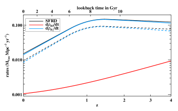
Figure 4.— Rates of gas flowing from one phase to another in an open box model with only stars, H₂ and HI (ignoring $\rho_{ext}\$). The SFRD (black curves) is an order of magnitude higher than $d\rho_{HI}/dt$ (red curve), forcing $d\rho_{H_{2}}/dt$ (blue curves) to be approximately equal to the SFRD, as in the closed box model. The two forms of the SFRD described in §2.1 are used: modified Sal A IMF (solid) and the Baldry & Glazebrook (2003) IMF (dashed). The derivatives of $\rho_{HI}\$and $\rho_{H_{2}}$ are negative, but the absolute values are plotted here.

3.3.2 $\rho_{ext}$

We are therefore forced to include a nonzero $d\rho_{ext}/dt$ term in the open box model. This component represents the ionized intergalactic gas at all temperatures and densities that can recombine to form H I within a Hubble time. Effectively, it is the ionized gas in the filaments of the cosmic web.

Note that some of the H I can become ionized and redistributed to the intergalactic medium at high enough temperatures and low densities such that this gas does not recombine in a Hubble time. Such gas can be ejected by means of supernovae, galactic winds or AGN. However, if we define $d\rho_{ext}/dt$ to be the net flow out of the ionized phase, then the gas that is fed back into the ionized state is implicitly included in our accounting. That is, any H I fed back into the ionized phase is made up by an equivalent increase in $d\rho_{ext}/dt$. If the total amount of ionized gas available is represented by $\Omega_{baryon}$ minus the total amount of baryons in galaxies, we may consider the ionized phase to be a nearly infinite reservoir of gas available to fuel star formation. Any gas ionized and added to that reservoir by star-formation and active galaxies is negligible.

To compute the $d\rho_{ext}/dt(t)$ required in the open box model to match the observations in §2, we start with an observed SFRD$(t)$ and $\rho_{HI}(t)$, and a guess for the form of the MGDR$(t)$ that is compatible with the data points from Tacconi et al. (2010) and Daddi et al. (2009). From these inputs, we compute $\rho_{H_{2}}(t)$ and its time derivative using $\rho_{H_{2}}(t)=\mathrm{SFRD}(t)/\mathrm{MGDR}(t)$. Combining $d\rho_{H_{2}}/dt$ with the observed SFRD$(t)$ and $d\rho_{HI}(t)/dt$ in Eq. (3) then gives $d\rho_{ext}/dt$. The results of this procedure are shown in Fig. 5.

To illustrate the expected range of possible values, we use two forms for the input MGDR (top left panel) and two forms for the input SFRD (black dashed curves in the right panel). We bracket the possible values for the MGDR on one side as constant using the measured value at $z=0$, and on the other as one that increases linearly to larger redshifts as suggested by the Tacconi et al. (2010) and Daddi et al. (2009) data points. For the SFRD, we use the smoothed piecewise fits from Hopkins & Beacom (2006) for the two extreme IMFs discussed in §2.1. We then calculate $d\rho_{H_{2}}/dt$, $d\rho_{ext}/dt$ and $\rho_{H_{2}}$ for each of the four possible combinations of MGDR and SFRD. The range of calculated values is indicated in Fig. 5 by plotting the minimum and maximum of the four curves for each calculated quantity.

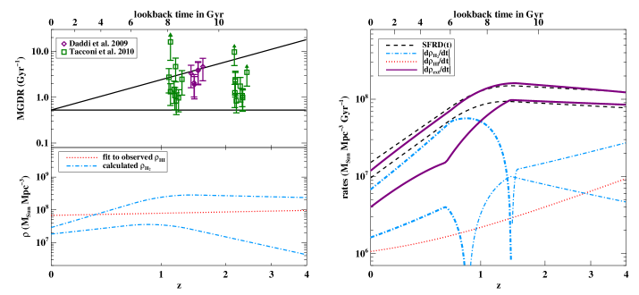
Figure 5.— Predictions of the open box model, calculated from combinations of the inputs: two forms of the MGDR (solid black lines in top left panel), two forms of the SFRD (dashed black lines in right panel) and the fit to the observations of $\rho_{HI}\$(red dotted line in bottom left panel). In the top left panel, we plot the MGDR points from Tacconi et al. (2010) (green squares) and Daddi et al. (2009) (purple diamonds) to constrain the guessed range of MGDR forms. The possible range of each of the calculated quantities, $d\rho_{H_{2}}/dt$, $d\rho_{ext}/dt$ and $\rho_{H_{2}}$, is shown by two lines illustrating the minimum and maximum curves from the four combinations of inputs. In the right panel, the absolute values of the rates are plotted: thicker lines indicate negative values.

In the bottom left panel, we note that the minimum $\rho_{H_{2}}$ curve lies below $\rho_{HI}\$at all times, and the maximum curve becomes larger than $\rho_{HI}\$at $z\sim 0.35$. The difference between the two curves is mostly the MGDR choice: the maximum curve corresponds to the higher SFRD and the flat MGDR, while the minimum curve corresponds to the lower SFR and the increasing MGDR (as expected from Eq. 1). All other combinations of MGDR and SFRD whould lie between these two curves. Because all of the molecular gas resides in galaxies, we require that the molecular gas mass in galaxies is larger, on average, at $z$ = 1-2, than is typical at $z$ = 0. The change in $\rho_{H_{2}}$ resulting from changing the SFRD is minor. Therefore, observations of $\rho_{H_{2}}$ at $z>0$ or the redshift at which $\rho_{H_{2}}=\rho_{HI}$ will constrain the form of the MGDR.

In the right panel, the absolute value of the rates is plotted, with a thicker line style used to indicate negative rates. The negative portions of the $d\rho_{H_{2}}/dt$ curves correspond to decreasing $\rho_{H_{2}}$ as we move forward in time towards $z=0$, as H₂ is converted into stars. The $d\rho_{ext}/dt$ curves are negative for the whole range of redshifts plotted, indicating a flow of external gas into the H I reservoir of galaxies. We note that the range of solutions for $d\rho_{ext}/dt$ does not deviate very much from the SFRD: roughly a factor of two at low redshifts for the minimum case. This is because the reservoirs of H₂ and H I are so small compared to what is required by the observed SFRD. Therefore, we conclude that the amount of inflow needed from this external gas, $d\rho_{ext}/dt$, is approximately equal to the SFRD. This observational conclusion is reinforced by cosmological simulations which find that star formation rates closely follow gas infall rates (Kereš et al., 2005; Dekel et al., 2009). Specifically, Kereš et al. (2009) calculate an upper limit on the external gas supply feeding galaxies that is only a factor of 2 higher than our predicted $d\rho_{ext}/dt$ curves and shows similar evolution with redshift.

4. Discussion

We have shown in §3.1 and §3.2 why the closed H₂ box model doesn’t work. Here we discuss the open box model of §3.3 and what this model predicts.

4.1. Variations in the SFRD

For the models in §3, we have extended the star formation rate prescription from Leroy et al. (2008) to mass densities averaged over Mpc scales: SFRD $\propto$ $\rho_{H_{2}}$. Some studies of galaxies with higher gas surface densities have found evidence for a steeper power law of SFRD $\propto\rho_{H_{2}}^{1.4}$ (Kennicutt, 1998; Wong & Blitz, 2002; Bouché et al., 2007). The choice of SFRD prescription at a given redshift depends on what type of galaxies dominate the SFRD at that redshift. At the present epoch, regular spiral galaxies, such as those studied by Leroy et al. (2008), seem to dominate the SFRD: Salim et al. (2007) finds that galaxies in the mass range $10^{9.3}<M_{*}<10^{10.6}M_{\odot}$ account for about half of the total SFRD. At higher redshifts, however, the BzK and BX/BM galaxies dominate the SFRD (see §2.2.2). These galaxies are more gas rich, and thus the $\rho_{H_{2}}^{1.4}$ prescription may be more appropriate.

For this paper, we have assumed the Leroy et al. (2008) prescription for the SFRD, but note that the power law may change at higher redshift because the dominant mode of star formation may change. This is equivalent to a change in the MGDR with time, a case we consider explicitly and probably contributes to the values of the MGDR found by Tacconi et al. (2010) and Daddi et al. (2009). If, for example, $SFRD=MGDR(0)\rho_{H_{2}}^{1.4}$ at higher redshift, then we would find $MGDR(z)=MGDR(0)\rho_{H_{2}}^{0.4}$ by forcing our prescription of $SFRD=MGDR\times\rho_{H_{2}}$. Thus as $\rho_{H_{2}}$ increases at higher redshift, an increase in the power law of the SFRD prescription will be manifested as an increase in the MGDR. An increase would tend to bring the MGDR closer to the upper bound in the top panel of Fig. 5, with the result that $\rho_{H_{2}}(z)$ would lie closer to the lower blue curve in the bottom panel in Fig. 5.

4.2. Stellar Recycling

Stellar recycling is an important component of any treatment of gas evolution in galaxies. Kennicutt et al. (1994), for example, suggest that gas returned to the ISM during stellar evolution can signficantly increase the gas depletion time in the Milky Way and in nearby galaxies. In the model presented here, we do not explicitly consider the effect of gas return to the ISM in Eqs. 1 and 3, but we argue that our formulation already accounts for stellar recycling due to the nature of the observed quantities we use as inputs. Most of the return of gas to the ISM comes from red giant stars (see e.g. Blitz 1997), and much of that is returned to the ISM in the form of molecules (Marengo, 2009). Even gas that is returned in other phases becomes largely molecular after each spiral arm passage, the timescale for which is $\sim 10^{8}$ yr in most galaxies, a timescle short compared to the rather long timescales we consider in this paper. Since the recycled gas is largely molecular, and any that isn’t is quickly returned to the molecular phase, we argue that observations of molecular gas already include the gas returned via stellar recycling. Therefore, this recycled component is included in our initial condition, $\rho_{H_{2}}(z=0)$, as well as the MGDR. Since we use the MGDR to relate SFRD and $\rho_{H_{2}}$ at each time step, stellar recycling is built into our model through these observations, so we need not include an explicit recycling term in our equations.

4.3. Behavior of $\rho_{H_{2}}(z)$

Although the exact shape of $\rho_{H_{2}}$ depends sensitively on the form of MGDR, we have bounded the behavior of $\rho_{H_{2}}$ by calculating what we take to be limiting cases in our open box model (Fig. 5). The $\rho_{H_{2}}$ curves all rise with increasing redshift, peaking around $z\sim 1-1.5$ at 1.5 to 10 times the value of $\rho_{H_{2}}$ today. After the peak, $\rho_{H_{2}}$ may fall off toward higher redshift if the MGDR is rather constant, or stay close to constant if the MGDR remains high. The prediction is less well constrained at higher redshifts. It is noteworthy that Tacconi et al. (2010) find that the gas disks they observe at $z=1$ and $z=2$ have considerably more molecular gas relative to the stars, typically about 30-50%, compared to $\sim 1-5\%$ for the Milky Way and nearby disk galaxies (Helfer et al., 2003). This trend is consistent with our estimates. Although there is some uncertainty in the H₂ masses of Tacconi et al. (2010) because of the uncertainty in the value of X_CO, there appears to be little doubt that the ratio of H₂ to stellar mass in the BzK and BX/BM galaxies is higher than typical values for similar galaxies at $z=0$. Due to the sensitivity of $\rho_{H_{2}}$ to the form of MGDR, future observations of $\rho_{H_{2}}$ or the ratio $\rho_{H_{2}}$/$\rho_{HI}\$at higher redshift would allow us to better constrain the evolution of MGDR, and reduce the area between the bounding curves of Fig. 5.

4.4. The Nature of $d\rho_{ext}/dt$

In our open box model, the H I reservoir, $\rho_{HI}$, is augmented by an inflow of gas from $\rho_{ext}\$at a rate of $10^{7}-10^{8}M_{\sun}\,{\rm Mpc^{-3}}$ Gyr^-1, depending on $z$. This high rate of inflow means that the gas being accreted is mostly ionized since the fraction of neutral hydrogen outside of the $\rho_{HI}\$reservoir is too small.

The $\rho_{HI}\$inferred from observations of DLA systems accounts for the H I associated with galactic disks. As mentioned in §3.3, O’Meara et al. (2007) find that systems with column density $\Sigma_{HI}<2\times 10^{20}$ cm^-2 account for $\approx 15\%$ of neutral hydrogen atoms at all $z<6$. Therefore, the fraction of H I outside DLA systems is about $15\%$, corresponding to roughly $1.5\times 10^{7}$ M${}_{\sun}\,{\rm Mpc^{-3}}$. For an average inflow rate of a few times $10^{7}$ M${}_{\sun}\,{\rm Mpc^{-3}}$ Gyr^-1 for the past 10 Gyr, this intergalactic H I could only account for ten percent of the total, at most. Therefore, the inflow of gas needed for fueling ongoing star formation represented by $d\rho_{ext}/dt$ must be almost completely ionized.

Recently, cold flows have been suggested as an important source of gas for galaxy formation and evolution (Kereš et al., 2005; Dekel & Birnboim, 2006). In these models, galactic disks in halos with $M\lesssim 10^{12}M_{\sun}$ are built up by direct accretion of cold gaseous streams from the cosmic web. For galaxies with larger masses, cold flows are also the dominant means of mass accretion, but different outcomes for individual galaxies depend on the epoch of inflow. If this picture is correct, our work implies that the cold flows must be almost entirely ionized.

The same is true if the gas needed to fuel star formation is brought in primarily through minor mergers. If this gas were in atomic form, it would be part of the inventory of atomic gas observed in the DLA systems, which we have shown in §3.3 to contribute negligibly to fueling the star formation at all redshifts up to $z=4$.

4.5. Cooling Times

The open box model requires $d\rho_{ext}/dt\sim SFRD$, or about $10^{7}$ to $10^{8}$ M${}_{\sun}\,{\rm Mpc^{-3}}$ Gy^-1. We use these numbers for $d\rho_{ext}/dt$ to calculate a cooling time for the gas in the context of two models for gas accretion onto galaxies: two-phase cooling of hot halo gas (Maller & Bullock, 2004) and cold flow accretion (Kereš & Hernquist, 2009).

We estimate the cooling time, $t_{cool}$, by taking

$$\frac{\rho_{gas}}{t_{cool}}\sim\dot{\rho}_{ext}\,,$$ (4)

where $\rho_{gas}$ is the average mass density of the cooling ionized gas smoothed over the appropriate volume (to be specified for each cooling model individually). We set $\rho_{gas}$ equal to $m_{H}n_{e}f$ where $n_{e}$ is the local number density of electrons and $f$ is the filling factor for the relevant volumes ($\bar{n}_{e}/n_{e}$). Combining this with the cooling time

$$t_{cool}\sim\frac{3k_{b}T}{2\Lambda(T)n_{e}}\,,$$ (5)

where $\Lambda(T)$ is the cooling function of the gas, gives

$$fn_{e}^{2}\sim\frac{3k_{b}T\dot{\rho}_{ext}}{2\Lambda(T)m_{H}}\,.$$ (6)

As a basis for comparison, we first estimate the filling factor $f$ for hot halos of $L_{*}$ galaxies out to the virial radius. We make the simplistic assumption that the universe is made up of $L_{*}$ galaxies with masses $M_{dyn}\sim 10^{12}$ M_☉ and circular velocities of $\sim 160$ km s^-1. Therefore, the virial radius, $R_{vir}=GM_{dyn}/v^{2}\sim 300$ kpc. We estimate the average number density in this simple universe composed of $L_{*}$ galaxies by dividing the total luminosity density, $\mathcal{L}$, by $L_{*}$. We use the r band values from Blanton et al. (2003) which calculates the galaxy luminosity function at $z\sim 0.1$ from SDSS data: $\mathcal{L}\approx 1.84\times 10^{8}$ h M_⊙ Mpc^-3, $L_{*}\approx 1.2\times 10^{10}$ h^-2 M_⊙. This yields $n_{L_{*}}\sim\mathcal{L}/L_{*}\sim 0.015$ h³ Mpc${}^{-3}\sim 5\times 10^{-3}$ Mpc^-3. More recent work on the luminosity function using SDSS DR6 yields similar results (Montero-Dorta & Prada, 2009). Therefore, in this simple universe, the filling factor for the $L_{*}$ galaxy halos is

$$f\sim n_{L_{*}}\frac{4}{3}\pi R_{vir}^{3}\sim 6\times 10^{-4}\,.$$ (7)

Maller & Bullock (2004) consider gas within the cooling radius of a halo, $R_{c}$, cooling via cloud fragmentation. This results in the formation of warm ($\sim 10^{4}$ K) clouds within the hot gas halo. In this model for the two-phase cooling of the hot halo gas, the relevant temperature for the gas is the virial temperature of the halo, $\sim 10^{6}$ K for a Milky Way type halo.

Kereš & Hernquist (2009) find that the majority of cold clouds that form around Milky Way type galaxies are the result of filamentary ”cold mode” accretion. Most of the gas does not reach the virial temperature of the halo, $\sim 10^{6}$ K, but rather cools from a maximum temperature of $\sim 10^{4}-10^{5}$ K.

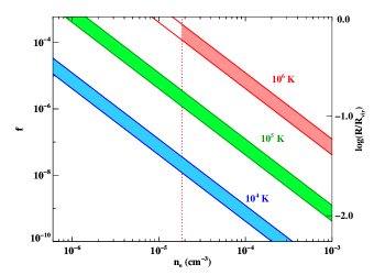
Figure 6.— Shaded regions show the allowed filling fraction $f$ and $n_{e}$ for three temperatures: $10^{4}$ K in blue, $10^{5}$ K in green and $10^{6}$ K in red. The axis on the right gives the radius of the relevant volumes as a fraction of the virial radius corresponding to the filling fraction $f$ in a simple universe filled with $L_{*}$ galaxies. At each temperature, the allowed region of $n_{e}$ vs $f$ space is calculated using the predicted range for the inflow rate at $z=0$: $d\rho_{ext}/dt=0.4-1.2\times 10^{7}$ M_☉ $\,{\rm Mpc^{-3}}$ Gyr^-1. The region is further bounded by the vertical dotted line at the value of $n_{e}$ corresponding to a cooling time equal to the age of the universe. This line is only plotted for the $10^{6}$ K gas: for the other two temperatures, the densities are very small and lie outside of the plotting range.

We examine the possible values for $n_{e}$ and $f$ in these two models by calculating $f$ as a function of $n_{e}$ for three temperatures: $10^{4}$ K and $10^{5}$ K for cold flow accretion and $10^{6}$ K for cooling from the hot halo. In Fig. 6, we plot $f$ versus $n_{e}$ for these three temperatues for the range of $d\rho_{ext}/dt$ at $z=0$ predicted by our open box model: $0.4-1.2\times 10^{7}$ M_☉ $\,{\rm Mpc^{-3}}$ Gyr^-1. The y-axis on the right side shows $\log(R/R_{virial})$ corresponding to $f$, where R is the radius of the relevant volume associated with an $L_{*}$ galaxy. The vertical dotted line indicates the value of $n_{e}$ at which the cooling time is equal to the age of the universe. We use the approximate form for $\Lambda(T)$ for mildly enriched gas ($Z=0.1$) from Maller & Bullock (2004) :

$$\Lambda(T)\simeq 2.6\times 10^{-23}\left(\frac{T}{10^{6}\ K}\right)^{-1}\ cm^{-3}\ erg\ s^{-1}$$ (8)

For the cold flow gas at $10^{4}$ K and $10^{5}$ K, the dotted lines where the cooling times equal the age of the universe are outside of the plotting range, so the minimum allowed value of $n_{e}$ is where $R\sim R_{virial}$: about $8\times 10^{-7}$ cm^-3 for the $10^{5}$ K gas and even smaller for the $10^{4}$ K gas. For the cooling hot halo gas at $10^{6}$ K, the condition that the cooling time be less than the age of the universe forces $n_{e}$ to be larger than about $2\times 10^{-5}$ cm^-3.

These calculations don’t put strong constraints on the density of the halo gas since the cooling times are so rapid for a large range of temperatures and densities. How the gas gets into the galaxies themselves will involve a more complete treatment including the effects of self-sheilding, which is beyond the scope of this paper.

4.6. Comparing $d\rho_{ext}/dt$ to Dark Matter Accretion Rate

The rate $d\rho_{ext}/dt$ inferred from our open box model provides an estimate for the average rate at which the baryonic fuel is required to make its way to a galactic disk in order to sustain the observed star formation, which largely occurs in the disk. A comparison of this rate with the mean rate of baryon accretion at the virial radius of the host dark matter halo will provide an estimate for the efficiency of converting the cosmological infalling baryons into stars. Many cooling and feedback processes obviously affect the fate of baryons after their infall onto the halo and whether they will reach the disk. In fact, much of the current research in galaxy formation modeling is aimed at understanding this transition. Our goal here is to estimate an overall ratio, as a function of redshift, of the baryon accretion rates at the virial radius and at the disk scale.

We begin with the dark matter accretion rate from McBride et al. (2009) and Fakhouri, Ma & Boylan-Kolchin (2010), which quantified the mass accretion histories of all dark matter halos with masses above $\sim 10^{10}$ M_⊙ in the two Millennium simulations of a $\Lambda$CDM universe (Springel et al., 2005; Boylan-Kolchin et al., 2009). An approximate function is provided for the average mass accretion rate as a function of redshift and halo mass (Fakhouri, Ma & Boylan-Kolchin, 2010):

$$\dot{M} = \beta\,M_{\odot}{\rm yr}^{-1}\left(\frac{M}{10^{12}M_{\odot}}\right)^{1.1}$$ (9)

$$\times(1+\gamma\,z)\sqrt{\Omega_{m}(1+z)^{3}+\Omega_{\Lambda}}\,.$$

where $(\beta,\gamma)=(25.3,1.65)$ for the median rate and (46.1, 1.11) for the mean rate, $\Omega_{m}$ and $\Omega_{\Lambda}$ are the present-day density parameters in matter and the cosmological constant, and $\Omega_{m}+\Omega_{\Lambda}$ is assumed to be unity (as in the Millennium simulation). The mean rate is $\sim 50$% higher than the median rate due to the long tail of halos with high accretion rates in the distribution. This $\dot{M}$ represents the average rate at which the mass in dark matter is being accreted through the virial radius of a halo. The mass growth comes in two forms in cosmological simulations: via mergers with other resolved halos (Fakhouri & Ma, 2009a), and via ”diffuse” accretion of non-halo material that is a combination of unresolved halos and unbound dark matter particles (Fakhouri & Ma, 2009b).

We convert $\dot{M}$ above into a mean accretion rate for the baryons, $\dot{M}_{b}$, by assuming a cosmic baryon-to-dark matter ratio of $f_{b}=\Omega_{b}/\Omega_{m}=1/6$. The result should provide a reasonable approximation for the mean rate of baryon mass that is entering the virial radius via mergers plus accretion of intergalactic gas. These infalling baryons are presumably in a mixture of forms: warm-hot ionized hydrogen gas of $10^{5}$ to $10^{7}$K, “cold” flows of $\sim 10^{4}$K (still ionized) gas, and H I, H₂, and stars brought in from merging galaxies. As discussed earlier, the majority of these baryons must be in the form of H II gas.

To compare $\dot{M}_{b}$ with the rate of external gas inflow, $\dot{\rho}_{ext}$ (§3.3), needed to account for the evolution of the observed star formation rates, we define

$$\alpha=\frac{d\rho_{ext}/dt}{f_{b}\dot{M}M(dn/dM)}\,,$$ (10)

where $M$ is the mass of the dark matter halo under consideration, $\dot{M}$ is calculated using Eq. (9), and $dn/dM$ is the (comoving) number density of dark matter halos with mass in the range of $M$ and $M+dM$. The parameter $\alpha$ represents the fraction of accreting baryons (at the virial radius) that must be converted into stars in our open box models.

The value of $\alpha$ can be estimated by combining the allowed range of $d\rho_{ext}/dt$ from Fig. 5 with the halo abundance $dn/dM$ from the Millennium simulation (Springel et al., 2005). Taking $f_{b}=1/6$ and $M=10^{12}$ M_⊙, we find the predicted $\alpha$ to be $\sim 70-100$% at $z\gtrsim 3$, $\sim 120-200$% at $z\sim 2$, and $\sim 30-90$% at $z=0$. We note here that several factors may contribute to the uncertainty in the alpha values. First, the distribution of $\dot{M}$ is broad at a given halo mass (see, e.g., Fig. 5 of Fakhouri, Ma & Boylan-Kolchin 2010), and we have simply used the mean value for a rough estimate of $\alpha$ here. Second, $\alpha$ depends on the halo mass appropriate for the population of galaxies that dominates the SFRD at a given redshift. Using a clustering analysis, Adelberger et al. (2005) find that BzK and BX/BM galaxies have halo masses of about $10^{12}$ M_☉, but the average value appropriate to our analysis may vary. However, since $\dot{M}\propto M^{1.1}$ and $Mdn/dm$ is approximately $\propto M^{-1}$, the mass dependence is weak, so alpha changes by a maximum of $\sim 20$% if we change the halo mass by a factor of 3. Third, since the $d\rho_{ext}/dt$ calculated in our open box model roughly traces the SFRD, the alpha values, especially around $z\sim 1-2$, will be affected by the exact form of the SFRD. Finally, the large alpha value at $z\sim 2$ may be reflecting a change in the fraction of baryons in the filaments at that redshift. Considering all the uncertainties, we make the conservative suggestion that the open box model requires a large fraction ($\sim 30-90$%) of the infalling baryons at the virial radius to be turned into stars from $z\sim 0-4$. This is consistent with the work of Dekel et al. (2009), which finds that the star formation rates in the typical ’star-forming galaxies’ at $z\sim 2$ are very close to the baryonic inflow rates from simulations.

Another way to estimate $\alpha$ is to compare the various $\dot{M}$ directly. At $z\sim 0$, the median baryon accretion rate from eq. (9) is $\dot{M}_{b}\sim 9$ M_⊙ yr^-1 for $2\times 10^{12}$ M_⊙ halos, and the measured star formation rate in the Milky Way ranges from $\dot{M}_{*}\sim 2$ M_⊙ yr^-1 to $\sim 4$ M_⊙ yr^-1 (Miller & Scalo, 1979; Diehl et al., 2006). These rates imply $\alpha\sim\dot{M}_{*}/\dot{M}_{b}\sim 25$ to 50% at $z\sim 0$. In addition, we can use the predicted $\dot{\rho}_{ext}$ from our open box models to estimate a mean conversion rate of external H II gas into stars per galaxy, $\dot{M}\sim\dot{\rho}_{ext}/n_{L_{*}}$. Taking $\dot{\rho}_{ext}\sim 10^{7}$ M${}_{\odot}{\rm Mpc}^{-3}$ Gyr^-1 from Fig. 5 and $n_{L_{*}}\sim 5\times 10^{-3}$ Mpc^-3 for the number density of $L_{*}$ galaxies today, we obtain a rate of $\sim 2$ M_⊙ yr^-1, which is consistent with the star formation rate in the Milky Way.

5. Summary and Conclusions

In this paper, we have built a quantitative model of gas consumption on cosmic scales based solely on observations. Using the observed the Star Formation Rate Density (SFRD), Molecular Gas Depletion Rate (MGDR), and volume averaged density of molecular hydrogen ($\rho_{H_{2}}$) and atomic hydrogen ($\rho_{HI}$) we have defined the cosmic molecular gas depletion problem and calculated the mass flow rates and densities of the star-forming gas back to $z\simeq 4$ needed to resolve it. Extrapolations further back in time are primarily limited by uncertainties in the SFRD. We find that:

• There are no models of gas consumption where the reservoir of gas is either only H₂ or both H I and H₂ that are compatible with the observations of molecular gas in the galaxies at $z\sim 2$ that produce the observed SFRD.

• Inflowing ionized intergalactic gas must provide most of the gas that turns into stars to times as early as $z\sim 4$. There is so little neutral gas inflow at all epochs, that the neutral gas ought to be considered more as a phase of cosmic gas flow than a reservoir of star forming gas.

• The rate of mass inflow from the ionized state to the atomic state roughly traces the star formation rate density. From $z\simeq 1-4$, the mass inflow rate is 1 - 2 $\times 10^{8}$ M_☉ Mpc^-3 Gyr^-1. At $z\lesssim 1$, the mass inflow rate varies linearly from about 0.5 $\times 10^{7}$ M_☉ Mpc^-3 Gyr^-1 at $z=0$ to about 1.5 $\times 10^{8}$ M_☉ Mpc^-3 Gyr^-1. At all redshifts, we find the mass inflow rate must be a significant fraction of the infalling rate at the virial radius, in agreement with simulations.

• For all models, the volume averaged density of H₂ increases from its present value by a factor of 1.5 to 10 at $z$ = 1 – 2 depending mostly on MGDR(t).

——————————————————————-

Appendix A Functional Form for the SFRD

The form for the SFRD used throughout the paper is a smoothed form of the piecewise fits from Hopkins & Beacom (2006). The original piecewise function is defined by intercept and slope a and b for $z<z_{1}$ and c and d for $z>z_{1}$ (we only consider $z<4$). The smoothed section is just a quadratic form in the $\log(1+z)$ vs $\log(SFRD)$ plane over a distance $2\Delta$ in $\log(1+z)$. We give the piecewise function for the SFRD below, with $x=\log(1+z)$ and $x_{1}=\log(1+z_{1})$.

$$\log\left(SFRD\right)=\left\{\begin{array}[]{lllr@{x}l}a&+&bx&0\leq&\leq x_{1}-\Delta\\ a&+&b(x_{1}-\Delta)+\frac{(d-b)}{4\Delta}\left(x^{2}-(x_{1}-\Delta)^{2}\right)\\ &+&\frac{1}{2}\left[b+d+(b-d)\frac{x_{1}}{\Delta}\right]\left(x-x_{1}+\Delta\right)&x_{1}-\Delta\leq&\leq x_{1}+\Delta\\ c&+&dx&x_{1}+\Delta\leq&\leq x_{max}\end{array}\right.$$ (A5)

In the table below, we give a,b,c,d and z1 for each of the two piecewise linear fits from Hopkins & Beacom (2006) (for the Modified Salpeter A IMF and the Baldry & Glazebrook (2003) IMF). To produce reasonable smoothing, we used $2\Delta=\log(1.5)$.

	Mod SalA IMF		BG 2003 IMF
a	-1.	82	-2.	02
b	3.	28	3.	44
c	-0.	724	-0.	930
d	-0.	26	-0.	26
$z_{1}$	1.	04	0.	97

Table 1Table of fit parameter values for the two piecewise linear fits from Hopkins & Beacom (2006): the Modified Salpeter A IMF and the Baldry & Glazebrook (2003) IMF.

References

- Adelberger et al. (2005) Adelberger, K. L., Steidel, C. C., Pettini, M., Shapley, A. E., Reddy, N. A., & Erb, D. K. 2005, ApJ, 619, 697
- Alves et al. (2007) Alves, J., Lombardi, M., & Lada, C. J. 2007, A&A, 462, L17
- Baldry & Glazebrook (2003) Baldry, I. K., & Glazebrook, K. 2003, ApJ, 593, 258
- Blaauw (1964) Blaauw, A. 1964, ARA&A, 2, 213
- Blanton et al. (2003) Blanton, M. R., et al. 2003, ApJ, 592, 819
- Blitz (1997) Blitz, L. 1997, IAU Symposium, 170, 11
- Boylan-Kolchin et al. (2009) Boylan-Kolchin, M., Springel, V., White, S. D. M., Jenkins, A. & Lemson, G. 2009, MNRAS, 398, 1150
- Bouché et al. (2007) Bouché, N., et al. 2007, ApJ, 671, 303
- Bouché et al. (2009) Bouché, N., et al. 2009, arXiv:0912.1858
- Burton et al. (1978) Burton, W. B., Liszt, H. S., & Baker, P. L. 1978, ApJ, 219, L6
- Carilli et al. (2002) Carilli, C. L., et al. 2002, AJ, 123, 1838
- Cazaux & Tielens (2004) Cazaux, S., & Tielens, A. G. G. M. 2004, ApJ, 604, 222
- Chabrier (2003) Chabrier, G. 2003, PASP, 115, 763
- Cole et al. (2001) Cole, S., et al. 2001, MNRAS, 326, 255
- Daddi et al. (2009) Daddi, E., et al. 2009, arXiv:0911.2776
- Dekel & Birnboim (2006) Dekel, A., & Birnboim, Y. 2006, MNRAS, 368, 2
- Dekel et al. (2009) Dekel, A., et al. 2009, Nature, 457, 451
- Diehl et al. (2006) Diehl, R. et al. 2006, Nature, 439, 45
- Fakhouri & Ma (2009a) Fakhouri, O., & Ma, C.-P. 2009a, MNRAS, 394, 1825
- Fakhouri & Ma (2009b) Fakhouri, O., & Ma, C.-P. 2009b, arXiv:0808.2471
- Fakhouri, Ma & Boylan-Kolchin (2010) Fakhouri, O., Ma, C.-P., Boylan-Kolchin, M. arXiv:1001.2304
- Förster Schreiber et al. (2009) Förster Schreiber, N. M., et al. 2009, ApJ, 706, 1364
- Gao & Solomon (2004) Gao, Y., & Solomon, P. M. 2004, ApJ, 606, 271
- Gil de Paz et al. (2007) Gil de Paz, A., et al. 2007, ApJS, 173, 185
- Grcevich & Putman (2009) Grcevich, J., & Putman, M. E. 2009, ApJ, 696, 385
- Hanish et al. (2006) Hanish, D. J., et al. 2006, ApJ, 649, 150
- Helfer et al. (2003) Helfer, T. T., Thornley, M. D., Regan, M. W., Wong, T., Sheth, K., Vogel, S. N., Blitz, L., & Bock, D. C.-J. 2003, ApJS, 145, 259
- Herbig & Kameswara Rao (1972) Herbig, G. H., & Kameswara Rao, N. 1972, ApJ, 174, 401
- Hernquist & Springel (2003) Hernquist, L., & Springel, V. 2003, MNRAS, 341, 1253
- Hippelein et al. (2003) Hippelein, H., et al. 2003, A&A, 402, 65
- Hollenbach & Salpeter (1971) Hollenbach, D., & Salpeter, E. E. 1971, ApJ, 163, 155
- Hopkins & Beacom (2006) Hopkins, A. M., & Beacom, J. F. 2006, ApJ, 651, 142
- Houck et al. (2007) Houck, J. R., Weedman, D. W., Le Floc’h, E., & Hao, L. 2007, ApJ, 671, 323
- Kennicutt et al. (1994) Kennicutt, R. C., Jr., Tamblyn, P., & Congdon, C. E. 1994, ApJ, 435, 22
- Kennicutt (1998) Kennicutt, R. C. 1998, ApJ, 498, 541
- Kennicutt et al. (2003) Kennicutt, R. C., Jr., et al. 2003, PASP, 115, 928
- Kereš & Hernquist (2009) Kereš, D., & Hernquist, L. 2009, ApJ, 700, L1
- Kereš et al. (2005) Kereš, D., Katz, N., Weinberg, D. H., & Davé, R. 2005, MNRAS, 363, 2
- Kereš et al. (2009) Kereš, D., Katz, N., Fardal, M., Davé, R., & Weinberg, D. H. 2009, MNRAS, 395, 160
- Lada (1992) Lada, E. A. 1992, ApJ, 393, L25
- Lah et al. (2007) Lah, P., et al. 2007, MNRAS, 376, 1357
- Lanzetta et al. (1995) Lanzetta, K. M., Wolfe, A. M., & Turnshek, D. A. 1995, ApJ, 440, 435
- Larson et al. (1980) Larson, R. B., Tinsley, B. M., & Caldwell, C. N. 1980, ApJ, 237, 692
- Leroy et al. (2008) Leroy, A. K., Walter, F., Brinks, E., Bigiel, F., de Blok, W. J. G., Madore, B., & Thornley, M. D. 2008, AJ, 136, 2782
- Madau et al. (1996) Madau, P., Ferguson, H. C., Dickinson, M. E., Giavalisco, M., Steidel, C. C., & Fruchter, A. 1996, MNRAS, 283, 1388
- Maller & Bullock (2004) Maller, A. H., & Bullock, J. S. 2004, MNRAS, 355, 694
- Marengo (2009) Marengo, M. 2009, Publications of the Astronomical Society of Australia, 26, 365
- McBride et al. (2009) McBride, J., Fakhouri, O., & Ma, C.-P. 2009, arXiv:0902.3659
- Miller & Scalo (1979) Miller, G. E., & Scalo, J. M. 1979, ApJS, 41, 513
- Montero-Dorta & Prada (2009) Montero-Dorta, A. D., & Prada, F. 2009, MNRAS, 399, 1106
- Motte et al. (1998) Motte, F., Andre, P., & Neri, R. 1998, A&A, 336, 150
- Myers (2008) Myers, P. C. 2008, ApJ, 687, 340
- Noterdaeme et al. (2009) Noterdaeme, P., Petitjean, P., Ledoux, C., & Srianand, R. 2009, A&A, 505, 1087
- Obreschkow & Rawlings (2009) Obreschkow, D., & Rawlings, S. 2009, MNRAS, 289
- O’Meara et al. (2007) O’Meara, J. M., Prochaska, J. X., Burles, S., Prochter, G., Bernstein, R. A., & Burgess, K. M. 2007, ApJ, 656, 666
- Omont et al. (1996) Omont, A., Petitjean, P., Guilloteau, S., McMahon, R. G., Solomon, P. M., & Pécontal, E. 1996, Nature, 382, 428
- Pei & Fall (1995) Pei, Y. C., & Fall, S. M. 1995, ApJ, 454, 69
- Prochaska & Wolfe (2009) Prochaska, J. X., & Wolfe, A. M. 2009, ApJ, 696, 1543
- Rao et al. (2006) Rao, S. M., Turnshek, D. A., & Nestor, D. B. 2006, ApJ, 636, 610
- Reddy et al. (2005) Reddy, N. A., Erb, D. K., Steidel, C. C., Shapley, A. E., Adelberger, K. L., & Pettini, M. 2005, ApJ, 633, 748
- Reddy et al. (2008) Reddy, N. A., Steidel, C. C., Pettini, M., Adelberger, K. L., Shapley, A. E., Erb, D. K., & Dickinson, M. 2008, ApJS, 175, 48
- Salim et al. (2007) Salim, S., et al. 2007, ApJS, 173, 267
- Sancisi et al. (2008) Sancisi, R., Fraternali, F., Oosterloo, T., & van der Hulst, T. 2008, A&A Rev., 15, 189
- Schaye et al. (2010) Schaye, J., et al. 2010, MNRAS, 402, 1536
- Schwartz et al. (1973) Schwartz, P. R., Wilson, W. J., & Epstein, E. E. 1973, ApJ, 186, 529
- Shu et al. (1987) Shu, F. H., Adams, F. C., & Lizano, S. 1987, ARA&A, 25, 23
- Springel et al. (2005) Springel, V., et al. 2005, Nature, 435, 629
- Steidel et al. (1999) Steidel, C. C., Adelberger, K. L., Giavalisco, M., Dickinson, M., & Pettini, M. 1999, ApJ, 519, 1
- Tacconi et al. (2008) Tacconi, L. J., et al. 2008, ApJ, 680, 246
- Tacconi et al. (2010) Tacconi, L., et. al. 2010, Nature, accepted
- Walter et al. (2008) Walter, F., Brinks, E., de Blok, W. J. G., Bigiel, F., Kennicutt, R. C., Thornley, M. D., & Leroy, A. 2008, AJ, 136, 2563
- Wolfe et al. (2005) Wolfe, A. M., Gawiser, E., & Prochaska, J. X. 2005, ARA&A, 43, 861
- Wong & Blitz (2002) Wong, T., & Blitz, L. 2002, ApJ, 569, 157
- Zwaan et al. (2005) Zwaan, M. A., Meyer, M. J., Staveley-Smith, L., & Webster, R. L. 2005, MNRAS, 359, L30
- Zwaan & Prochaska (2006) Zwaan, M. A., & Prochaska, J. X. 2006, ApJ, 643, 675