Ioffe Times in DIS from a Dipole Model Fit

Abstract:

We present a study of Ioffe times in deep inelastic electron-proton scattering. We deduce ‘experimental’ Ioffe-time distributions from the small-$x$ HERA data as described by a particular colour-dipole-model fit. We show distributions for three representative $\gamma^{*}p$ c. m. energies $W$ and various values of the photon virtuality $Q^{2}$. These distributions are rather broad for transversely and very narrow for longitudinally polarised virtual photons. The Ioffe times for $W=150~{}\mbox{GeV}$, for example, range from around $10^{3}$ fm for $Q^{2}=1~{}\mbox{GeV}^{2}$ to around 10 fm for $Q^{2}=100~{}\mbox{GeV}^{2}$. Based on our results we discuss consequences for the limitations of applicability of the dipole picture.

1 Introduction

In this article we shall present a quantitative study of the space-time structure of deep inelastic electron- and positron-proton scattering (DIS)

$$e^{\pm}+p\rightarrow e^{\pm}+X$$ (1)

as measured extensively in HERA experiments [1, 2, 3, 4, 5]. We shall be concerned with the kinematic region where only exchange of a virtual photon between the leptons and the hadrons matters. Thus, as usual, with the reaction (1) we study in fact the absorption of a virtual photon on the proton

$$\gamma^{\ast}+p\rightarrow X\,.$$ (2)

The total cross section for (2) is, apart from kinematic factors, given by the imaginary part of the amplitude for forward Compton scattering of a virtual photon on the proton,

$$\gamma^{*}+p\rightarrow\gamma^{*}+p\,.$$ (3)

The study of the space-time structure of this process has a long history going back to the discussions of the vector-meson-dominance (VMD) model in the 1960s and in particular to articles by Gribov et al. [6] and Ioffe [7]. In [7] the question was posed where and when the initial virtual photon is absorbed, that is, where it fluctuates into ‘hadronic stuff’ and where the ‘hadronic stuff’ fluctuates back to give the final virtual photon. In this article we shall give quantitative answers to this question, as far as the region of small $x$ is concerned, using the HERA data. In fact we shall use a fit to these data in a particular colour dipole model.

Let us first make some more historical remarks. It is an old idea that the scattering of a highly-energetic photon on a hadron may essentially be considered as a strong interaction process where the photon acts in some way as a hadron. Vector mesons as intermediary particles in the coupling of photons to nucleons were introduced in [8, 9, 10] in order to understand properties of the electromagnetic form factors. An important role was assigned to vector mesons in strong interactions in [11]. Then in [12] the vector-meson-dominance model was proposed. There it is assumed that whenever a photon couples to hadrons it first converts to the vector mesons $\rho$, $\omega$, $\phi$ (proposed / known at the time) with universal coupling constants. These vector mesons have then normal hadronic reactions. The VMD model was rather successful in describing many results from photon-hadron reactions. For reviews see, for instance, [13, 14]. But the results from deep inelastic scattering presented problems. Indeed, in [15] a simple form of this VMD picture was applied to DIS and predictions were made which, however, were subsequently disproven by experiments. This led to the formulation of the concept of generalized vector meson dominance, see [16, 14, 17] and references therein. The key idea in these descriptions is that the photon fluctuates into a series of vector mesons which subsequently scatter off the proton. Quite obviously, the lifetime of the fluctuation of the photon into a vector meson needs to be sufficiently long for that picture to be consistent.

The colour dipole model [18, 19, 20] builds on similar ideas but is motivated to a large extent by perturbative QCD. In this picture the reaction (2) is viewed as a two-step process. In the first step the photon splits into a quark-antiquark pair which represents the colour dipole. Subsequently that pair scatters on the proton, this second step being a purely hadronic reaction. For the applicability of the dipole model it is crucial that the lifetime of the fluctuation of the photon into the colour dipole is much larger than the typical timescale of the dipole-proton interaction. In the context of the dipole picture the lifetime of the dipole fluctuation is usually referred to as the Ioffe time. We may note in parentheses, however, that Ioffe in his original paper [7] was concerned with a somewhat different time as we shall comment on below. It is the aim of the present paper to study the distribution of Ioffe times and their dependence on the kinematical parameters of the photon-proton scattering process using the HERA data on DIS.

The splitting of a photon of high enough virtuality $Q^{2}$ into a quark-antiquark pair can be calculated in perturbation theory. The subsequent scattering of the colour dipole off the proton, on the other hand, is a genuinely nonperturbative process. Therefore, this second step of the $\gamma^{*}p$ scattering process needs to be described by suitable models. A variety of such models has been constructed, see [21, 22, 23] for some prominent examples and [24, 25] for overviews. These models are very successful in describing the structure functions measured at HERA.

But despite the impressive phenomenological success of dipole models there are some caveats. In [26, 27] the foundations of the dipole picture were examined in detail. It was shown that a number of assumptions and approximations is required to arrive at the dipole picture. These results naturally raise the question about the range of validity of these approximations and assumptions. In [28, 29] it was found that already the general formulae of the standard dipole approach allow one to derive stringent bounds on various ratios of structure functions. These bounds were then used to determine the kinematic region where the dipole picture is compatible with the data. An important point in this connection concerns the variables on which the dipole-proton cross section depends. The natural variables were found to be $r$, the transverse size of the dipole, and $W$, the c. m. energy of the dipole-proton scattering. Using this functional dependence for the dipole-proton cross section we obtained the following result: For $\gamma^{\ast}p$ c. m. energies $W$ in the range of 60 to 240 GeV the standard dipole picture fails to be compatible with the HERA data for photon virtualities $Q^{2}$ larger than about $100$ to $200$ GeV² [29]. Clearly, these large virtualities correspond to relatively short Ioffe times. In the present paper we want to study this relation between Ioffe times and the kinematical parameters in more detail by calculating the distribution of Ioffe times and the corresponding contributions to the structure functions for given values of $Q^{2}$ and $W$.

Let us, therefore, consider the reaction (2) at high c. m. energy in the proton rest system. The virtual photon $\gamma^{\ast}$ of $4$-momentum $q=(q^{0},\boldsymbol{q})$ fluctuates into a quark and antiquark of $4$-momenta $k=(k^{0},\boldsymbol{k})$ and $k^{\prime}=(k^{\prime 0},\boldsymbol{k}^{\prime})$ respectively, where $3$-momentum is conserved, $\boldsymbol{q}=\boldsymbol{k}+\boldsymbol{k}^{\prime}$. Energy, however, is not conserved. Instead, there is an energy mismatch

$$\Delta E=k^{0}+k^{\prime 0}-q^{0}$$ (4)

between the quark-antiquark pair and the virtual photon. According to the uncertainty relation such a fluctuation cannot live longer than the time

$$\tau=\frac{1}{\Delta E}=\frac{1}{k^{0}+k^{\prime 0}-q^{0}}\,.$$ (5)

In the following we shall call $\tau$ the Ioffe time for the initial $\gamma^{*}$. Discussions of Ioffe time distributions in the context of the operator product expansion can be found in [30]. In [31] the Ioffe-time structure of the gluon distribution function in the double logarithmic approximation was considered.

In applications of the dipole model one frequently finds simple estimates for Ioffe times, and if they turn out to be of the order of several femtometers or larger this is taken as justification for using the dipole model. But the actual situation is more involved. We shall find that even for a fixed kinematical point for reaction (2) one has a whole distribution of Ioffe times. In fact, the $\gamma^{\ast}p$ total absorption cross section is most conveniently obtained from the imaginary part of the forward scattering amplitude for the reaction (3), $\gamma^{\ast}p\to\gamma^{\ast}p$. As a consequence, we shall have to deal with two Ioffe times, one for the initial state $\gamma^{\ast}$ and one for the final state $\gamma^{\ast}$. Both times have distributions which also depend on the polarisation, transverse or longitudinal, of the $\gamma^{\ast}$. We shall calculate such distributions in the following from the HERA data using a phenomenological dipole model which describes the data quite well. We shall choose the model of Golec-Biernat and Wüsthoff (GBW) [21] for this purpose.

In section 2 we review the relevant formulae of the dipole picture and define the $\Delta E$ and Ioffe time $\tau$ distributions in this framework. In section 3 we recall the basics of the GBW model for the dipole cross section. We then present numerical results for the $\Delta E$ and the corresponding Ioffe-time distributions. Our conclusions are drawn in section 4. In two appendices we present the details of our calculations.

2 Ioffe time and $\Delta E$ distributions in the dipole picture

We use the standard formulae for the kinematics and for the definitions of structure functions of deep inelastic electron- and positron-proton scattering (1), see for instance [32]. For momentum transfers squared $Q^{2}\lesssim 1000~{}\text{GeV}^{2}$ it is sufficient to consider only the exchange of a virtual photon between the lepton and the proton in (1). Thus, the reaction which we shall study in the following is the absorption of a virtual photon $\gamma^{\ast}$ on the proton,

$$\gamma^{\ast}(q)+p(p)\rightarrow X(p^{\prime})\,,$$ (6)

where we indicate the $4$-momenta in brackets. The c.m. energy for this reaction is denoted by $W$, the virtuality of the $\gamma^{\ast}$ by $Q^{2}$. For these and for Bjorken’s scaling variable $x$ we have

$$\begin{split}W^{2}&=(p+q)^{2}\,,\\ Q^{2}&=-q^{2}\,,\\ x&=\frac{Q^{2}}{2p\cdot q}=\frac{Q^{2}}{W^{2}+Q^{2}-m_{p}^{2}}\,.\end{split}$$ (7)

The proton in (6) is supposed to be unpolarised, but the virtual photon can have transverse or longitudinal polarisation. The corresponding total cross sections are $\sigma_{T}(W,Q^{2})$ and $\sigma_{L}(W,Q^{2})$, respectively. The structure function $F_{2}$ is

$$F_{2}(W,Q^{2})=\frac{Q^{2}}{4\pi^{2}\alpha_{\rm em}}\left[\sigma_{T}(W,Q^{2})+\sigma_{L}(W,Q^{2})\right](1-x)+\mathcal{O}\left(\frac{m_{p}^{2}}{W^{2}}\right)\,.$$ (8)

For small Bjorken-$x$, $x\ll 1$, this simplifies to

$$F_{2}(W,Q^{2})=\frac{Q^{2}}{4\pi^{2}\alpha_{\mathrm{em}}}\left[\sigma_{T}(W,Q^{2})+\sigma_{L}(W,Q^{2})\right]\,.$$ (9)

In the following we shall use this simpler relation since we shall only consider data for $x\ll 1$. In order to obtain the standard dipole model for the cross sections $\sigma_{T,L}$ we can relate them first to the imaginary part of the virtual Compton forward scattering amplitude,

$$\gamma^{*}(q)+p(p)\rightarrow\gamma^{*}(q)+p(p)\,.$$ (10)

The latter is then represented as the initial $\gamma^{\ast}$ splitting into a $q\bar{q}$ pair, this pair scattering on the proton, and the $q\bar{q}$ subsequently fusing into the final state $\gamma^{\ast}$, see figure 1. Note that this figure is to be read from right to left in order to be in complete analogy with the occurrence of the various factors in the amplitudes in the equations below.

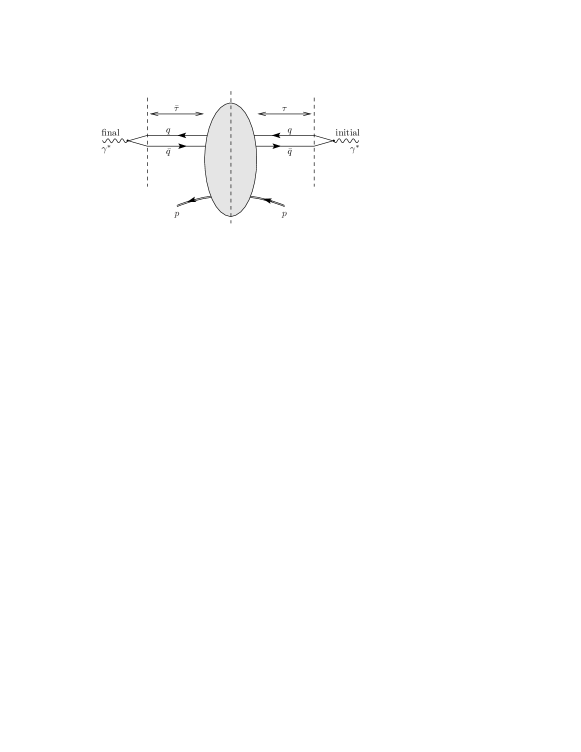
Figure 1: Basic diagram for the description of the cross sections $\sigma_{T,L}$ of $\gamma^{\ast}p$ scattering in the standard dipole approach

With the assumptions spelled out in detail in section 6 of [27] the diagram of figure 1 gives

$$\sigma_{T}(W,Q^{2}) =\sum_{q}\int\mathrm{d}^{2}r\int_{0}^{1}\mathrm{d}\alpha\sum_{\lambda,\lambda^{\prime}}\left(\psi_{\lambda\lambda^{\prime}}^{(q)\,\pm}(\alpha,\boldsymbol{r},Q)\right)^{\ast}\,\hat{\sigma}^{(q)}(r,W)\,\psi_{\lambda\lambda^{\prime}}^{(q)\,\pm}(\alpha,\boldsymbol{r},Q)\,,$$ (11)

$$\sigma_{L}(W,Q^{2}) =\sum_{q}\int\mathrm{d}^{2}r\int_{0}^{1}\mathrm{d}\alpha\sum_{\lambda,\lambda^{\prime}}\left(\psi_{\lambda\lambda^{\prime}}^{(q)\,L}(\alpha,\boldsymbol{r},Q)\right)^{\ast}\,\hat{\sigma}^{(q)}(r,W)\,\psi_{\lambda\lambda^{\prime}}^{(q)\,L}(\alpha,\boldsymbol{r},Q)\,.$$ (12)

Here $\alpha$ is the longitudinal momentum fraction of the $\gamma^{\ast}$ carried by the quark, $\boldsymbol{r}$ is the vector in transverse position space from the antiquark to the quark, $r=|\boldsymbol{r}|$, and $\lambda$ and $\lambda^{\prime}$ are the helicities of $q$ and $\bar{q}$, respectively. The total cross section for the scattering of the $q\bar{q}$ pair on the proton is denoted by $\hat{\sigma}^{(q)}$, the wave functions for transversely and longitudinally polarised virtual photons by $\psi_{\lambda\lambda^{\prime}}^{(q)\,\pm}$ and $\psi_{\lambda\lambda^{\prime}}^{(q)\,L}$, respectively. For the explicit form of these wave functions see appendix A. A sum over all contributing quark flavours $q$ is to be performed.

However, the standard representation of the photon wave functions in terms of longitudinal momentum fraction $\alpha$ and transverse position $\boldsymbol{r}$ is not suitable for a discussion of Ioffe-time distributions. To study them we have to go to longitudinal and transverse momentum space. There we can directly read off the energy mismatch between the $\gamma^{*}$ and the $q\bar{q}$ pair, both for the initial and the final states. Let us, therefore, consider first the splitting of the initial $\gamma^{*}$ into a $q\bar{q}$ pair in momentum space. We have 3-momentum but not energy conservation at this splitting. Taking this into account we define the $4$-momentum of the quark, $k$, and that of the antiquark, $k^{\prime}$, by

$$\boldsymbol{k} =\alpha\boldsymbol{q}+\boldsymbol{k}_{T}\,, k^{0} =\sqrt{\boldsymbol{k}^{2}+m_{q}^{2}}\,,$$

$$\boldsymbol{k}^{\prime} =(1-\alpha)\boldsymbol{q}-\boldsymbol{k}_{T}\,, k^{\prime 0} =\sqrt{\boldsymbol{k}^{\prime 2}+m_{q}^{2}}\,.$$ (13)

Here, in essence, $\alpha\in[0,1]$. The precise $\alpha$-range is discussed in appendix B. Then the photon wave functions in momentum space are easily calculated. For a derivation see for example [27]. We give the results in appendix A both in the – in leading order in $\alpha_{\rm s}$ and $\alpha_{\rm em}$ – exact and in the approximate form which is usually used in the dipole model fits. The approximation involves in particular neglecting terms such as $(\boldsymbol{k}_{T}^{2}+m_{q}^{2})/(\alpha^{2}\boldsymbol{q}^{2})$ and $(\boldsymbol{k}_{T}^{2}+m_{q}^{2})/((1-\alpha)^{2}\boldsymbol{q}^{2})$ with respect to 1. However, for some given $\left|\boldsymbol{q}\right|$ those terms become non-negligible if $k_{T}=|\boldsymbol{k}_{T}|$ is large or if $\alpha$ is close to $\mathrm{𝟎}$ or $1$. If relevant contributions to some observable depend on the photon wave functions in this kinematical region the above approximation could become invalid. This is potentially important when considering distributions in the Ioffe times, in particular for short Ioffe times. We shall calculate the distributions with and without the above approximation in order to quantify this effect.

The photon wave functions in transverse position space are related by a Fourier transformation to their momentum space representations

$$\psi_{\lambda\lambda^{\prime}}^{(q)\,\pm,L}(\alpha,\boldsymbol{r},Q)=\int\frac{\mathrm{d}^{2}k_{T}}{(2\pi)^{2}}\,e^{i\boldsymbol{k}_{T}\boldsymbol{r}}\tilde{\psi}_{\lambda\lambda^{\prime}}^{(q)\,\pm,L}(\alpha,\boldsymbol{k}_{T},Q)\,.$$ (14)

The next step is to insert the representation (14) for the wave functions for both the initial and final state photon into (11) and (12). This gives

$$\sigma_{T}(W,Q^{2}) =\sum_{q,\lambda,\lambda^{\prime}}\int\!\mathrm{d}\alpha\frac{\mathrm{d}^{2}\bar{k}_{T}}{(2\pi)^{2}}\frac{\mathrm{d}^{2}k_{T}}{(2\pi)^{2}}\left(\tilde{\psi}^{(q)\,\pm}_{\lambda\lambda^{\prime}}(\alpha,\boldsymbol{\bar{k}}_{T},Q)\right)^{\ast}\tilde{\hat{\sigma}}^{(q)}(\boldsymbol{k}_{T}-\boldsymbol{\bar{k}}_{T},W)\tilde{\psi}^{(q)\,\pm}_{\lambda\lambda^{\prime}}(\alpha,\boldsymbol{k}_{T},Q)\,,$$ (15)

$$\sigma_{L}(W,Q^{2}) =\sum_{q,\lambda,\lambda^{\prime}}\int\!\mathrm{d}\alpha\frac{\mathrm{d}^{2}\bar{k}_{T}}{(2\pi)^{2}}\frac{\mathrm{d}^{2}k_{T}}{(2\pi)^{2}}\left(\tilde{\psi}^{(q)\,L}_{\lambda\lambda^{\prime}}(\alpha,\boldsymbol{\bar{k}}_{T},Q)\right)^{\ast}\tilde{\hat{\sigma}}^{(q)}(\boldsymbol{k}_{T}-\boldsymbol{\bar{k}}_{T},W)\tilde{\psi}^{(q)\,L}_{\lambda\lambda^{\prime}}(\alpha,\boldsymbol{k}_{T},Q)\,.$$ (16)

Here we denote the Fourier transform of the dipole-proton cross section by

$$\tilde{\hat{\sigma}}^{(q)}(\boldsymbol{k}_{T},W)=\int\mathrm{d}^{2}r\,e^{i\boldsymbol{k}_{T}\boldsymbol{r}}\,\hat{\sigma}^{(q)}(r,W)\,.$$ (17)

The four-momenta of the quark and antiquark in the initial state dipole are given in (2). For the quark and antiquark in the final state dipole we denote the 4-momenta by $\bar{k}$ and $\bar{k}^{\prime}$, respectively. They are obtained from (2) with the replacements $k\to\bar{k}$, $k^{\prime}\to\bar{k}^{\prime}$, and $\boldsymbol{k}_{T}\to\bar{\boldsymbol{k}}_{T}$. Note that $\alpha$ stays the same.

We recall now the definition of the energy mismatches $\Delta E$ for the initial $\gamma^{\ast}$ splitting to $q\bar{q}$ and $\Delta\bar{E}$ for the final $q\bar{q}$ fusing to $\gamma^{\ast}$:

$$\Delta E =k^{0}+k^{\prime 0}-q^{0}\,,$$ (18)

$$\Delta\bar{E} =\bar{k}^{0}+\bar{k}^{\prime 0}-q^{0}\,.$$ (19)

The corresponding Ioffe times are

$$\tau =\frac{1}{\Delta E}\,,$$ (20)

$$\bar{\tau} =\frac{1}{\Delta\bar{E}}\,.$$ (21)

We have $\Delta E\geq 0$ and $\Delta\bar{E}\geq 0$ which implies also $\tau\geq 0$ and $\bar{\tau}\geq 0$.

From (15) and (16) we see that the cross sections $\sigma_{T}$ and $\sigma_{L}$ involve the superpositions of amplitudes of various $\Delta E$ in the initial and various $\Delta\bar{E}$ in the final state. Therefore, we define the joint distributions in $\eta=\Delta E$ and $\bar{\eta}=\Delta\bar{E}$ by

$$\begin{split}\frac{\partial^{2}\sigma_{T,L}(W,Q^{2},\eta,\bar{\eta})}{\partial\eta\,\partial\bar{\eta}}=\sum_{q}\sum_{\lambda,\lambda^{\prime}}\int\!\mathrm{d}\alpha&\int\!\frac{\mathrm{d}^{2}\bar{k}_{T}}{(2\pi)^{2}}\int\!\frac{\mathrm{d}^{2}k_{T}}{(2\pi)^{2}}\left(\tilde{\psi}^{(q)\,\pm,L}_{\lambda\lambda^{\prime}}(\alpha,\boldsymbol{\bar{k}}_{T},Q)\right)^{\ast}\,\delta(\bar{\eta}-\Delta\bar{E})\\ &\times\tilde{\hat{\sigma}}^{(q)}(\boldsymbol{k}_{T}-\boldsymbol{\bar{k}}_{T},W)\,\delta(\eta-\Delta E)\,\tilde{\psi}^{(q)\,\pm,L}_{\lambda\lambda^{\prime}}(\alpha,\boldsymbol{k}_{T},Q)\,.\end{split}$$ (22)

Note that these distributions are real-valued (see (A)) but for $\eta\neq\bar{\eta}$ they need not be positive. For specific dipole models we can now calculate $\tilde{\hat{\sigma}}^{(q)}$ and evaluate the two-dimensional distributions (22). However, one-dimensional distributions are more easily visualised. Thus, in the following we shall study how the sum of $\Delta E$ and $\Delta\bar{E}$

$$\Delta E_{+}=\Delta E+\Delta\bar{E}$$ (23)

is distributed. We, therefore, define

$$\frac{\partial\sigma_{T,L}(W,Q^{2},\Delta E_{+})}{\partial\Delta E_{+}} =\int_{0}^{\infty}\!\mathrm{d}\eta\int_{0}^{\infty}\!\mathrm{d}\bar{\eta}\,\frac{\partial^{2}\sigma_{T,L}(W,Q^{2},\eta,\bar{\eta})}{\partial\eta\,\partial\bar{\eta}}\,\delta(\Delta E_{+}-\eta-\bar{\eta})$$ (24)

and the Ioffe time corresponding to $\Delta E_{+}$ by

$$\tau_{+}=\frac{1}{\Delta E_{+}}=\frac{\tau\bar{\tau}}{\tau+\bar{\tau}}\,.$$ (25)

The quantity $2\tau_{+}$ is called the ‘harmonic mean’ of $\tau$ and $\bar{\tau}$ [33]. From (25) we get then $\tau\geq\tau_{+}$ and $\bar{\tau}\geq\tau_{+}$. That is, for given $\tau_{+}$ only individual Ioffe times $\tau$ and $\bar{\tau}$ which are larger or equal to $\tau_{+}$ contribute. At this point we may also note that Ioffe in his original paper [7] considered the time between the initial $\gamma^{*}$ fluctuating into ‘hadronic stuff’ and this ‘stuff’ fluctuating back to the final $\gamma^{*}$. In our calculation this corresponds to the time $\tau+\bar{\tau}$. For given $\tau_{+}$ we have $\tau+\bar{\tau}\geq 4\tau_{+}$.

In the next section we shall present numerical results for normalised distributions in $\ln\Delta E_{+}$ respectively $\ln\tau_{+}=-\ln\Delta E_{+}$. First we shall study these distributions for $F_{2}$,

$$\frac{\Delta E_{+}}{F_{2}}\frac{\partial F_{2}}{\partial\Delta E_{+}}=\frac{\Delta E_{+}}{\sigma_{T}+\sigma_{L}}\left(\frac{\partial\sigma_{T}}{\partial\Delta E_{+}}+\frac{\partial\sigma_{L}}{\partial\Delta E_{+}}\right)\,.$$ (26)

It is also of interest to study the distributions in the Ioffe time $\tau_{+}$ and in $\Delta E_{+}$ for the contributions of individual quark flavours to $\sigma_{T}$ and $\sigma_{L}$. For this we define $\sigma_{T}^{(q)}$, $\sigma_{L}^{(q)}$, and $\partial^{2}\sigma_{T,L}^{(q)}/\partial\eta\partial\bar{\eta}$ as in (15), (16), and (22), respectively, but omitting the sum over the quark flavours $q$ on the r.h.s. Then we define $\partial\sigma_{T,L}^{(q)}/\partial\Delta E_{+}$ in analogy to (24). The corresponding normalised distributions in $\ln\Delta E_{+}$ are given by

$$\frac{\Delta E_{+}}{\sigma_{T,L}^{(q)}}\frac{\partial\sigma_{T,L}^{(q)}}{\partial\Delta E_{+}}\,.$$ (27)

3 Results

In this section we present results for the distributions in $\Delta E_{+}$ and in Ioffe times $\tau_{+}$ in DIS. To evaluate (26) and (27) we have to choose a specific dipole-model fit to the data since we need the values for the dipole-proton cross sections $\hat{\sigma}^{(q)}$; see (11), (12), and (17). In the following we choose to work with the model constructed by Golec-Biernat and Wüsthoff [21]. This GBW model describes the $F_{2}$ data from HERA quite well. Whether it also describes the longitudinal structure function $F_{L}$ is not yet clear since the first $F_{L}$ measurements from HERA [34] are not precise enough to draw firm conlusions. The dipole cross section of this model is given for quark flavour $q$ by

$$\hat{\sigma}_{\mathrm{GBW}}^{(q)}(r,x)=\sigma_{0}\left[1-\exp\left(-\frac{r^{2}}{4r_{0}^{2}(\tilde{x})}\right)\right],$$ (28)

where

$$r_{0}^{2}(\tilde{x})=\frac{1}{Q_{0}^{2}}\left(\frac{\tilde{x}}{x_{0}}\right)^{\lambda}\,,\qquad\tilde{x}=x\left(1+\frac{4m_{q}^{2}}{Q^{2}}\right)\,.$$ (29)

We choose their parameter set which includes the charm quark, $Q_{0}=1~{}\mbox{GeV}$, $\sigma_{0}=29.12~{}\mbox{mb}$, $\lambda=0.277$, $x_{0}=0.41\cdot 10^{-4}$, $m_{q}=0.14~{}\mbox{GeV}$ for $q=u,d,s$, and $m_{c}=1.5~{}\mbox{GeV}$. The $b$-quark contributions are neglected in this fit.

The GBW dipole cross section $\hat{\sigma}_{\rm GBW}^{(q)}$ depends on $r$ and Bjorken-$x$, and therefore not only on $r$ and $W$ but also on $Q^{2}$, see (7). As was discussed in [27, 28] the natural and – in our opinion – correct energy variable for the dipole cross section $\hat{\sigma}^{(q)}$ is $W$, and $\hat{\sigma}^{(q)}$ should actually be independent of $Q^{2}$. A dependence on $x$ requires additional assumptions which appear difficult to justify. We will discuss the problem of choosing the correct energy variable in more detail elsewhere. For the present considerations, however, this issue how the $\hat{\sigma}^{(q)}$ depend on the kinematic variables is not of prime relevance since we only need a dipole model fit to the data at given values of these variables.

Now it is relatively straightforward to calculate the Fourier transform of $\hat{\sigma}_{\mathrm{GBW}}^{(q)}$, to insert it as well as the expressions for the $\gamma^{*}$ wave functions from appendix A in (15), (16) and (22), and to obtain the numerical results for the distributions in $\ln\Delta E_{+}=-\ln\tau_{+}$. The calculational details are presented in appendix B. The results for the normalised $F_{2}$ distribution (26) are shown for $\gamma^{*}p$ c. m. energies $W=70$, $150$ and $220~{}\mbox{GeV}$ and a number of $Q^{2}$ values in figure 2.

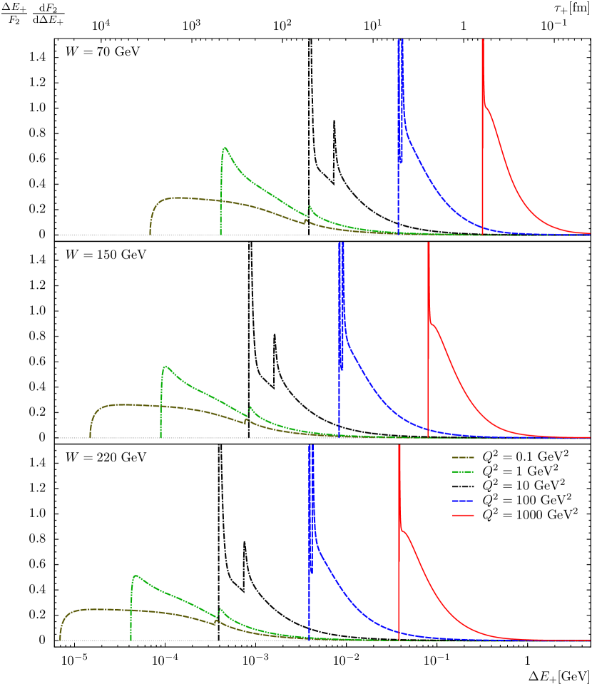
Figure 2: The normalised $F_{2}$ distribution (26) in the joint dipole-energy mismatch $\Delta E_{+}$ for the GBW model with charm. Supplementary to the $\Delta E_{+}$ values the corresponding values for the Ioffe times $\tau_{+}$ are denoted for the abscissa.

In figure 3 we present the normalised distributions in $\ln\Delta E_{+}=-\ln\tau_{+}$ for $\sigma_{T}^{(q)}$ and $\sigma_{L}^{(q)}$ for the individual quark flavours separately, here for the energy $W=150~{}\mbox{GeV}$.

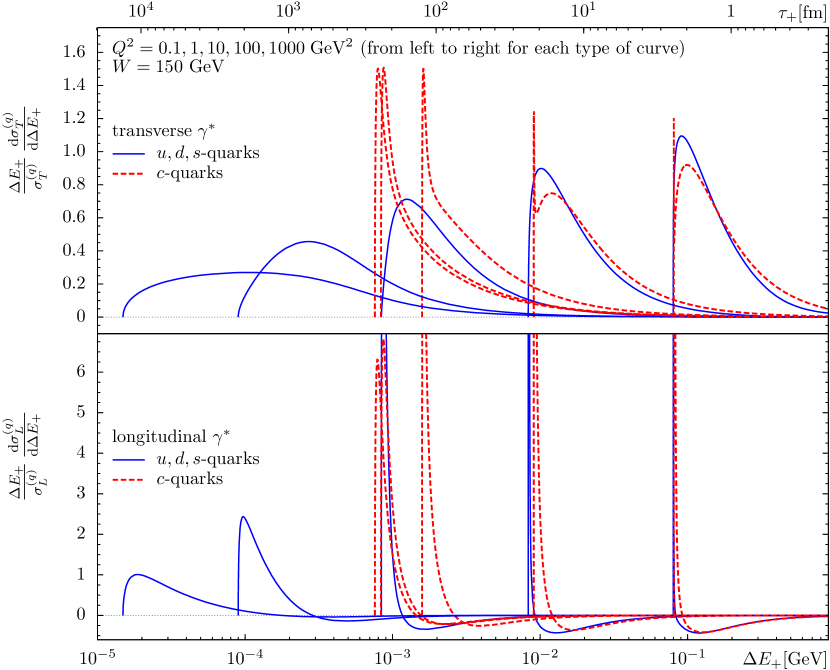
Figure 3: The normalised $\sigma_{T}^{(q)}$ and $\sigma_{L}^{(q)}$ distributions (27) in the joint dipole-energy mismatch $\Delta E_{+}$ respectively Ioffe time $\tau_{+}$ for the GBW model with charm.

In the calculations for figures 2 and 3 the full expressions (A) and (A) are used for the photon wave functions rather than their high energy and small-$k_{T}$ approximation. Also, we integrate over the full range in $\alpha$ which is slightly bigger than $[0,1]$, see (63). We have studied the effect of the high energy approximation (41)-(44) for the photon wave functions as well as of restricting the $\alpha$ integration range to $[0,1]$. The Ioffe-time distributions in figures 2 and 3 are essentially unaltered when performing the $\alpha$ integration only over $[0,1]$. The $\alpha$ range specified by (63) is only slightly larger than $[0,1]$ and no sufficiently strong enhancement of the integrand compensates for this fact in the kinematical ranges considered here. As expected, effects in the Ioffe-time distributions from the high energy and small-$k_{T}$ approximation for the photon wave functions become larger for increasing $\Delta E_{+}$. These deviations would alter the curves of figures 2 and 3 to an amount that is clearly visible only in the high $Q^{2}$ and small $W$ cases. However, for all distributions they are still small enough to be safely omitted from our further discussions here. We stress that this result is not obvious, since the interplay of the high energy and small-$k_{T}$ approximation and the dipole energy mismatch is non-trivial in the longitudinal-momentum endpoint regions.

Let us now discuss the main features of the curves in figures 2 and 3. We first note that due to the normalisation of the curves in figure 3 one cannot deduce from them the relative importance of light quarks and the $c$ quark in $F_{2}$. This information is obtained from figure 2 where the secondary peaks in the individual curves are due to the $c$-quark contributions. The peaks seen in figures 2 and 3 are not infinitely sharp. We analysed their structure using an enlarged $\Delta E_{+}$ scale and find them to be smooth finite maxima in all cases.

The curves in figure 3 clearly exhibit the respective thresholds due to the kinematical lower bounds for the various quark flavours $q$,

$$\Delta E_{+,\text{min}}=2\left(\sqrt{\boldsymbol{q}^{2}+4m_{q}^{2}}-q^{0}\right)=2\left(\sqrt{\boldsymbol{q}^{2}+4m_{q}^{2}}-\sqrt{\boldsymbol{q}^{2}-Q^{2}}\right)\,,$$ (30)

see (51) and (23). The quantities $\Delta E_{+,\text{min}}$ are shown in the left graph of figure 4 for light quarks as functions of $Q^{2}$ for $W=70$, $150$ and $220~{}\mbox{GeV}$.

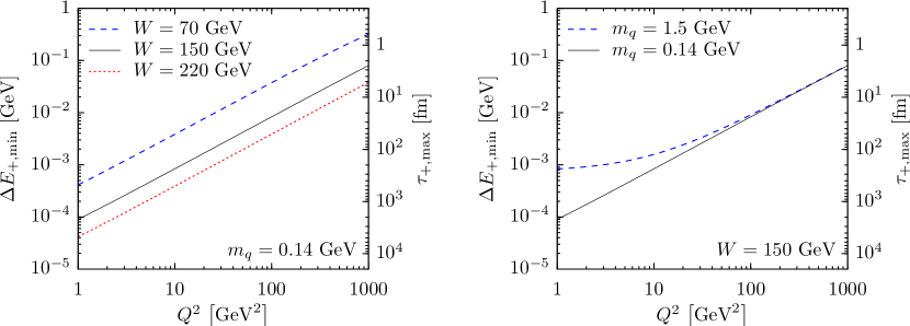
Figure 4: Minimal energy mismatch $\Delta E_{+,\text{min}}$ and corresponding maximal Ioffe time $\tau_{+,\text{max}}$ of the $\gamma^{*}$–dipole transition as a function of the photon virtuality $Q^{2}$. The curves are for different values of the energy $W$ in the case of light quarks (left graph) and for different quark masses in the case $W=150~{}\mbox{GeV}$ (right graph).

In the right graph of figure 4 we show $\Delta E_{+,\text{min}}$ as a function of $Q^{2}$ for $W=150\,\mbox{GeV}$ for the light quark mass and for the charm mass. From figure 3 we see that the $\Delta E_{+}$ distributions for transverse $\gamma^{\ast}$ polarisation are significantly broader than those for longitudinal $\gamma^{\ast}$ polarisation. For both polarisation types the distributions become narrower for increasing values of $Q^{2}$. The distributions for longitudinal polarisation have negative parts which is alright, see the discussion after (22).

The normalised distributions in $\tau_{+}$ respectively $\Delta E_{+}$ shown in figure 2 are obtained from the DIS small-$x$ data from HERA, using a specific dipole-model fit. In order to test the model dependence we have also investigated another fit of the GBW type and find compatible results.

From figure 2 we can clearly see that the Ioffe times decrease with increasing $Q^{2}$ at fixed $W$. At fixed $Q^{2}$ the Ioffe times increase with increasing $W$. The distributions are always rather broad. At $W=70~{}\mbox{GeV}$ and $Q^{2}=100~{}\mbox{GeV}^{2}$, for example, the upper cutoff for the Ioffe time $\tau_{+}$ is 5 fm and, indeed, the peaks of the distribution are there. But we have also significant contributions for $\tau_{+}$ down to 1 fm. As stressed already in the introduction, for the dipole picture to be a valid description of DIS the Ioffe times have to be appreciably larger than the typical interaction time $\tau_{\rm had}$ of the dipole with the proton. As an estimate of the latter we take the electromagnetic radius of the proton $\tau_{\rm had}\approx r_{p}\approx 1~{}\mbox{fm}$. A necessary condition for both dipole lifetimes $\tau$ and $\bar{\tau}$ (see (20), (21)) to be much larger than $\tau_{\rm had}$ is thus $\Delta E_{+}\ll 1/\tau_{\rm had}$ or, equivalently,

$$\tau_{+} \gg\tau_{\rm had}\approx 1~{}\text{fm}\,.$$ (31)

If this condition is violated for a relevant portion of the $\tau_{+}$ distribution of $F_{2}$ the applicability of the dipole model is questionable for the kinematical point under consideration.

From figure 2 we see that for $W=70~{}\mbox{GeV}$ the typical Ioffe times $\tau_{+}$ are reasonably above $1$ fm for all $Q^{2}\leq 100$ GeV². There, the necessary separation condition (31) is satisfied. However, for $Q^{2}=1000$ GeV² we see that the separation condition (31) is clearly violated, since the complete $\tau_{+}$ distribution lies at $\tau_{+}<1~{}\mbox{fm}$. For $W=150~{}\mbox{GeV}$ the distributions are shifted to larger values of $\tau_{+}$. But still for $Q^{2}=1000~{}\mbox{GeV}^{2}$ the $\tau_{+}$ distribution only starts at $\tau_{+}\approx 2.5~{}\mbox{fm}$ and extends well below $\tau_{+}=1~{}\mbox{fm}$. For $W=220~{}\mbox{GeV}$ and $Q^{2}=1000~{}\mbox{GeV}^{2}$ the situation is similar with the maximal $\tau_{+}\approx 5~{}\mbox{fm}$. Therefore, we must conclude from our study of Ioffe-time distributions in DIS that the basic separation condition of time scales (31) is violated in the HERA energy range $W=70$ to $220~{}\mbox{GeV}$, for $Q^{2}$ values of hundred to several hundred GeV².

4 Conclusions

We have calculated Ioffe-time distributions for DIS in the HERA energy range in the framework of the dipole model. As a convenient fit to the data we used the Golec-Biernat-Wüsthoff parametrisation of the dipole-proton cross section. We have obtained Ioffe-time distributions for $\gamma^{*}p$ c. m. energies $W=70$, $150$ and $220~{}\mbox{GeV}$ and $Q^{2}$ values ranging from $0.1$ to $1000~{}\mbox{GeV}^{2}$. A basic requirement for the dipole model to make sense is that the Ioffe times at the kinematic point considered are much larger than the hadronic timescale $\tau_{\rm had}\approx 1~{}\mbox{fm}$. We find that typical Ioffe times are large with respect to this hadronic scale for $Q^{2}\leq 100$ GeV², such that no inconsistencies arise there. However, at photon virtuality $Q^{2}=1000$ GeV² typical Ioffe times are of similar order as or smaller than the hadronic scale, which violates the standard assumption for the validity of the dipole picture. Thus, we find that in the HERA energy range the dipole picture starts to lack physical justification for $Q^{2}$ values in the hundred to several hundred GeV² range.

Note that we come to this conclusion here using a GBW fit to the HERA data where the dipole-proton cross section is assumed to depend on $r$ and Bjorken $x$. In [29] we have investigated the limits of applicability of the dipole model to the HERA data using the – in our opinion correct – dependence of the dipole-proton cross section on $r$ and $W$. From figure 9 of [29] we see that, nevertheless, we found a very similar $Q^{2}$ range for the applicability of the dipole model. The upper limits for $Q^{2}$ as obtained from this figure range from about $120~{}\mbox{GeV}^{2}$ at $W=70~{}\mbox{GeV}$ to about $180~{}\mbox{GeV}^{2}$ at $W=220~{}\mbox{GeV}$. These are strict bounds in the sense that the data cannot be fitted for a larger $Q^{2}$ range with a non-negative dipole-proton cross section depending on $r$ and $W$. In our present work we find that even if a fit to the data with a dipole-proton cross section depending on $r$ and Bjorken $x$ is possible also for higher values of $Q^{2}$ its physical meaning may become questionable there since the Ioffe times become too short. For very small $Q^{2}$ values, $Q^{2}\leq 2~{}\mbox{GeV}^{2}$ say, the Ioffe times shown in figure 2 are very large. Nevertheless, this does not immediately imply that the standard dipole model is without problems there. As discussed in [27, 28, 29] the lowest order expressions for the photon wave functions are expected to become unreliable in this kinematic region.

In summary, we have calculated ‘experimental’ Ioffe-time distributions from the small-$x$ HERA data as described by a GBW dipole-model fit. We have studied their dependence on the energy $W$ and on the photon virtuality $Q^{2}$. The Ioffe-time distributions of the cross sections are found to be rather broad for transversely and very narrow for longitudinally polarised virtual photons. Accordingly, the Ioffe-time distributions of $F_{2}$ are always rather broad.

Appendix A Photon wave functions and energy mismatch $\Delta E$

In this appendix we collect the formulae of the dipole model which are relevant for our calculations. The assumptions needed to arrive at the standard dipole picture of DIS are spelled out in detail in section 6.2 of [27]. One obtains the following – in leading order in $\alpha_{\rm s}$ and $\alpha_{\rm em}$ exact – expressions for the momentum-space wave functions of the virtual photon from (52) and (58) of [27],

$$\tilde{\psi}^{(q)\,\pm}_{\lambda\lambda^{\prime}}(\alpha,\boldsymbol{k}_{T},Q)= \mp\frac{N}{\sqrt{2}}Q_{q}\frac{1}{\Delta E}\frac{\left|\boldsymbol{q}\right|}{2\pi k^{0}2k^{\prime 0}}\frac{2}{\sqrt{k^{0}+m_{q}}\sqrt{k^{\prime 0}+m_{q}}}$$

$$\times\Big{[}\pm\left((k^{0}+m_{q})(k^{\prime 0}+m_{q})-\alpha(1-\alpha)\boldsymbol{q}^{2}\right)\delta_{\lambda,\lambda^{\prime}}\delta_{\lambda,\pm\frac{1}{2}}$$ (32)

$$\quad\quad+e^{\pm i\phi_{k}}k_{T}\left|\boldsymbol{q}\right|\delta_{\lambda,-\lambda^{\prime}}\big{(}\alpha\delta_{\lambda,\pm\frac{1}{2}}-(1-\alpha)\delta_{\lambda,\mp\frac{1}{2}}\big{)}\pm e^{\pm i2\phi_{k}}k_{T}^{2}\delta_{\lambda,\lambda^{\prime}}\delta_{\lambda,\mp\frac{1}{2}}\Big{]}\,,$$

$$\tilde{\psi}^{(q)\,L}_{\lambda\lambda^{\prime}}(\alpha,\boldsymbol{k}_{T},Q)= -NQ_{q}\frac{1}{\Delta E}\frac{\left|\boldsymbol{q}\right|}{2\pi k^{0}2k^{\prime 0}}\frac{\left|\boldsymbol{q}\right|-q^{0}}{Q}\frac{1}{\sqrt{k^{0}+m_{q}}\sqrt{k^{\prime 0}+m_{q}}}$$

$$\times\Big{[}\big{(}k_{T}^{2}+(k^{0}+m_{q}+\alpha\left|\boldsymbol{q}\right|)(k^{\prime 0}+m_{q}+(1-\alpha)\left|\boldsymbol{q}\right|)\big{)}\delta_{\lambda,-\lambda^{\prime}}$$

$$\quad\quad+e^{-i(\operatorname{sign}\lambda)\phi_{k}}(\operatorname{sign}\lambda)(k^{0}-k^{\prime 0}-(1-2\alpha)\left|\boldsymbol{q}\right|)k_{T}\delta_{\lambda,\lambda^{\prime}}\Big{]}\,.$$ (33)

Here $q$ denotes the quark flavours, $Q_{q}$ their charges in units of the proton charge $e=\sqrt{4\pi\alpha_{\rm em}}$. The number of colours is $N_{c}=3$. The momenta $k$ and $k^{\prime}$ of the quark and antiquark, respectively, are defined in (2), and we have $k_{T}=|\boldsymbol{k}_{T}|$ and $\phi_{k}=\arg(k_{T1}+ik_{T2})$. The normalisation factor is

$$N=-2\sqrt{N_{c}\pi}\,e\,\sqrt{\alpha(1-\alpha)}\,.$$ (34)

Note that the wave functions satisfy the following relations

$$\left(\tilde{\psi}^{(q)\,\pm}_{\lambda\lambda^{\prime}}(\alpha,\boldsymbol{k}_{T},Q)\right)^{*} =\tilde{\psi}^{(q)\,\pm}_{\lambda\lambda^{\prime}}(\alpha,\boldsymbol{k}_{T}^{R},Q)\,,$$ (35)

$$\left(\tilde{\psi}^{(q)\,L}_{\lambda\lambda^{\prime}}(\alpha,\boldsymbol{k}_{T},Q)\right)^{*} =\tilde{\psi}^{(q)\,L}_{\lambda\lambda^{\prime}}(\alpha,\boldsymbol{k}_{T}^{R},Q)\,,$$ (36)

where

$$\boldsymbol{k}_{T}^{R}=\left(\begin{array}[]{c}k_{T1}\\ -k_{T2}\end{array}\right)\,.$$ (37)

With (35) and (36) we can show that the distributions defined in (22) are real-valued. Indeed, from (17) we find that $\tilde{\hat{\sigma}}^{(q)}(\boldsymbol{k}_{T},W)$ is independent of the direction of $\boldsymbol{k}_{T}$ and, therefore,

$$\left(\tilde{\hat{\sigma}}^{(q)}(\boldsymbol{k}_{T},W)\right)^{*} =\tilde{\hat{\sigma}}^{(q)}(-\boldsymbol{k}_{T},W)$$

$$=\tilde{\hat{\sigma}}^{(q)}(\boldsymbol{k}_{T}^{R},W)\,.$$ (38)

We then get from (22)

$$\left(\frac{\partial^{2}\sigma_{T,L}(W,Q^{2},\eta,\bar{\eta})}{\partial\eta\,\partial\bar{\eta}}\right)^{*} =\sum_{q}\sum_{\lambda,\lambda^{\prime}}\int\!\mathrm{d}\alpha\int\!\frac{\mathrm{d}^{2}\bar{k}_{T}}{(2\pi)^{2}}\int\!\frac{\mathrm{d}^{2}k_{T}}{(2\pi)^{2}}\,\tilde{\psi}^{(q)\,\pm,L}_{\lambda\lambda^{\prime}}(\alpha,\boldsymbol{\bar{k}}_{T},Q)\,\delta(\bar{\eta}-\Delta\bar{E})$$

$$\hskip 28.45274pt\times\left(\tilde{\hat{\sigma}}^{(q)}(\boldsymbol{k}_{T}-\boldsymbol{\bar{k}}_{T},W)\right)^{*}\delta(\eta-\Delta E)\left(\tilde{\psi}^{(q)\,\pm,L}_{\lambda\lambda^{\prime}}(\alpha,\boldsymbol{k}_{T},Q)\right)^{*}$$

$$=\sum_{q}\sum_{\lambda,\lambda^{\prime}}\int\!\mathrm{d}\alpha\int\!\frac{\mathrm{d}^{2}\bar{k}_{T}}{(2\pi)^{2}}\int\!\frac{\mathrm{d}^{2}k_{T}}{(2\pi)^{2}}\left(\tilde{\psi}^{(q)\,\pm,L}_{\lambda\lambda^{\prime}}(\alpha,\boldsymbol{\bar{k}}_{T}^{R},Q)\right)^{*}\delta(\bar{\eta}-\Delta\bar{E})$$

$$\hskip 28.45274pt\times\tilde{\hat{\sigma}}^{(q)}(\boldsymbol{k}_{T}^{R}-\boldsymbol{\bar{k}}_{T}^{R},W)\,\delta(\eta-\Delta E)\,\tilde{\psi}^{(q)\,\pm,L}_{\lambda\lambda^{\prime}}(\alpha,\boldsymbol{k}_{T}^{R},Q)$$

$$=\frac{\partial^{2}\sigma_{T,L}(W,Q^{2},\eta,\bar{\eta})}{\partial\eta\,\partial\bar{\eta}}\,.$$ (39)

In the high energy and small-$k_{T}$ limit

$$\left|\boldsymbol{q}\right|\to\infty\,,\quad Q^{2}\ll|\boldsymbol{q}^{2}|\,,\quad\frac{\boldsymbol{k}_{T}^{2}+m_{q}^{2}}{\alpha^{2}\boldsymbol{q}^{2}}\ll 1\,,\quad\frac{\boldsymbol{k}_{T}^{2}+m_{q}^{2}}{(1-\alpha)^{2}\boldsymbol{q}^{2}}\ll 1\,,$$ (40)

the photon wave functions simplify to

$$\tilde{\psi}^{(q)\,\pm}_{\lambda\lambda^{\prime}}(\alpha,\boldsymbol{k}_{T},Q) =\frac{\sqrt{2N_{c}\alpha_{\rm em}}Q_{q}}{\alpha(1-\alpha)Q^{2}+k_{T}^{2}+m_{q}^{2}}\Big{[}m_{q}\delta_{\lambda,\lambda^{\prime}}\delta_{\lambda,\pm\frac{1}{2}}$$

$$\quad\qquad\pm k_{T}e^{\pm i\phi_{k}}\delta_{\lambda,-\lambda^{\prime}}\left(\alpha\delta_{\lambda,\pm\frac{1}{2}}-(1-\alpha)\delta_{\lambda,\mp\frac{1}{2}}\right)\Big{]}\,,$$ (41)

$$\tilde{\psi}^{(q)\,L}_{\lambda\lambda^{\prime}}(\alpha,\boldsymbol{k}_{T},Q) =-\frac{2\sqrt{N_{c}\alpha_{\rm em}}Q_{q}}{\alpha(1-\alpha)Q^{2}+k_{T}^{2}+m_{q}^{2}}\,\alpha(1-\alpha)Q\,\delta_{\lambda,-\lambda^{\prime}}\,.$$ (42)

Inserting the expressions (41), (42) into the Fourier transform (14) yields the standard formulae for the wave functions in longitudinal momentum and transverse position space (see again [27] for a detailed derivation)

$$\psi_{\lambda\lambda^{\prime}}^{(q)\pm}(\alpha,\boldsymbol{r},Q) =\frac{\sqrt{N_{c}}}{\sqrt{2}\pi}\sqrt{\alpha_{\rm em}}\,Q_{q}\left\{\pm\,ie^{\pm i\phi_{r}}\,\delta_{\lambda^{\prime},-\lambda}\left[\alpha\,\delta_{\lambda,\pm\frac{1}{2}}-(1-\alpha)\,\delta_{\lambda,\mp\frac{1}{2}}\right]\epsilon_{q}K_{1}(\epsilon_{q}r)\right.$$

$$\quad\left.\hskip 85.35826pt+\,m_{q}\,\delta_{\lambda,\pm\frac{1}{2}}\delta_{\lambda^{\prime},\lambda}K_{0}(\epsilon_{q}r)\right\}\,,$$ (43)

$$\psi_{\lambda\lambda^{\prime}}^{(q)L}(\alpha,\boldsymbol{r},Q) =-\frac{\sqrt{N_{c}}}{\pi}\sqrt{\alpha_{\rm em}}\,Q_{q}Q\,\alpha(1-\alpha)\,\delta_{\lambda^{\prime},-\lambda}\,K_{0}(\epsilon_{q}r)\,.$$ (44)

Here $\phi_{r}=\arg(r_{1}+ir_{2})$,

$$\epsilon_{q}=\sqrt{\alpha(1-\alpha)Q^{2}+m_{q}^{2}}\,,$$ (45)

and $K_{0,1}$ are the modified Bessel functions. Hence we have in the high energy and small-$k_{T}$ limit (40) for the $\gamma^{*}p$ cross sections the results (11) and (12), that is,

$$\sigma_{T,L}(W,Q^{2})=\sum_{q}\int\mathrm{d}^{2}r\int^{1}_{0}\mathrm{d}\alpha\sum_{\lambda,\lambda^{\prime}}\left|\psi^{(q)+,L}_{\lambda\lambda^{\prime}}(\alpha,\boldsymbol{r},Q)\right|^{2}\hat{\sigma}^{(q)}(r,W)$$ (46)

with

$$\!\sum_{\lambda,\lambda^{\prime}}\left|\psi_{\lambda\lambda^{\prime}}^{(q)+}(\alpha,\boldsymbol{r},Q)\right|^{2} =\frac{N_{c}}{2\pi^{2}}\,\alpha_{\rm em}Q_{q}^{2}\left\{\left[\alpha^{2}+(1-\alpha)^{2}\right]\epsilon_{q}^{2}[K_{1}(\epsilon_{q}r)]^{2}+m_{q}^{2}[K_{0}(\epsilon_{q}r)]^{2}\right\},$$ (47)

$$\!\sum_{\lambda,\lambda^{\prime}}\left|\psi_{\lambda\lambda^{\prime}}^{(q)L}(\alpha,\boldsymbol{r},Q)\right|^{2} =\frac{2N_{c}}{\pi^{2}}\,\alpha_{\rm em}Q_{q}^{2}Q^{2}[\alpha(1-\alpha)]^{2}[K_{0}(\epsilon_{q}r)]^{2}\,.$$ (48)

For the calculation of $\sigma_{T}$ above we can choose either of the two polarisations, $+$ or $-$ in (46), since they lead to the same cross section. We have chosen the $+$ polarisation here.

Let us now discuss some basic properties of the energy mismatch $\Delta E$ (18) which follow directly from the kinematics of the $\gamma^{*}\to q\bar{q}$ splitting. Similar considerations then apply to $\Delta\bar{E}$ in (19). Explicitly we obtain from (18) and (2) for quark flavour $q$

$$\Delta E(k_{T},\alpha) =\sqrt{\alpha^{2}\boldsymbol{q}^{2}+k_{T}^{2}+m_{q}^{2}}+\sqrt{(1-\alpha)^{2}\boldsymbol{q}^{2}+k_{T}^{2}+m_{q}^{2}}-q^{0}\,.$$ (49)

Figure 5 shows the dependence of $\Delta E(k_{T},\alpha)$ on the absolute value $k_{T}$ of the quark’s transverse momentum (left graph) and on its longitudinal momentum fraction $\alpha$ for the case of light quarks (right graph). We note that $\Delta E(k_{T},\alpha)$ strongly peaks at the longitudinal momentum endpoints and rises monotonically with the transverse momentum.

Figure 5: Energy mismatch $\Delta E$ of the $\gamma^{*}$ dipole transition as a function of the absolute value $k_{T}$ of the quark’s transverse momentum (left graph) and of its longitudinal momentum fraction $\alpha$ (right graph). The parameters are $W=150$ GeV, $Q^{2}=10$ GeV², $m_{q}=0.14$ GeV. For the left graph we have chosen $\alpha=1/2$ and for the right graph $k_{T}=1$ GeV, respectively. The dotted line shows the absolute minimum $\Delta E_{\text{min,abs}}$ for the given external kinematics, that is, $\Delta E$ at $k_{T}=0$ and $\alpha=1/2$.

At fixed $\alpha$ the energy mismatch becomes minimal for $k_{T}=0$:

$$\Delta E_{\text{min}}(\alpha)=\Delta E(0,\alpha)=\sqrt{\alpha^{2}\boldsymbol{q}^{2}+m_{q}^{2}}+\sqrt{(1-\alpha)^{2}\boldsymbol{q}^{2}+m_{q}^{2}}-q^{0}\,.$$ (50)

The absolute minimum of $\Delta E$ is reached at $k_{T}=0$, $\alpha=1/2$,

$$\Delta E_{\text{min,abs}}=\Delta E(0,1/2)=\sqrt{\boldsymbol{q}^{2}+4m_{q}^{2}}-q^{0}\,.$$ (51)

That is, we have

$$\Delta E(k_{T},\alpha)\geq\Delta E_{\text{min}}(\alpha)\geq\Delta E_{\text{min,abs}}\geq 0\,,$$ (52)

where the last inequality is strict for all $Q^{2}>0$. Thus we see that there is an a priori minimal value for the energy mismatch $\Delta E$ at a given kinematical point and for given quark flavour. Figure 4 in section 3 shows twice this minimal energy mismatch.

Appendix B Some technical details of the calculation

In this appendix we give the details of the calculations for the $\Delta E$ distributions (22), (24), and the corresponding quantities for individual quark flavours $q$. We use the Golec-Biernat-Wüsthoff model [21] which describes the $F_{2}$ data from HERA quite well. The dipole cross section of this model is given in (28) and (29). We point out again that the dipole cross sections $\hat{\sigma}_{\mathrm{GBW}}^{(q)}$ depend not only on $W$ but also on $Q^{2}$ through the $x$ dependence. We use the GBW model nevertheless, since we shall only be concerned with specific kinematic values of $W$ and $Q^{2}$ for which we study Ioffe-time distributions. We shall not compare structure functions at the same $W$ and different $Q^{2}$ values, where the choice of energy variable is essential, see [28, 29].

The Fourier transformation (17) of $\hat{\sigma}_{\mathrm{GBW}}^{(q)}(r,x)$ (28) gives

$$\tilde{\hat{\sigma}}_{\mathrm{GBW}}^{(q)}(\boldsymbol{k}_{T},x)=\sigma_{0}\left[(2\pi)^{2}\delta^{(2)}(\boldsymbol{k}_{T})-4\pi r_{0}^{2}\exp(-r_{0}^{2}k_{T}^{2})\right]\,.$$ (53)

Our aim is to calculate the $\Delta E_{+}$ distributions for the various quark-flavour contributions to $\sigma_{T}$ and $\sigma_{L}$. We have

$$\begin{split}\frac{\partial^{2}\sigma_{T,L}^{(q)}(W,Q^{2},\eta,\bar{\eta})}{\partial\eta\,\partial\bar{\eta}}=\sum_{\lambda,\lambda^{\prime}}\int\!\mathrm{d}\alpha&\int\!\frac{\mathrm{d}^{2}\bar{k}_{T}}{(2\pi)^{2}}\int\!\frac{\mathrm{d}^{2}k_{T}}{(2\pi)^{2}}\left(\tilde{\psi}^{(q)\,\pm,L}_{\lambda\lambda^{\prime}}(\alpha,\boldsymbol{\bar{k}}_{T},Q)\right)^{\ast}\,\delta(\bar{\eta}-\Delta\bar{E})\\ &\times\tilde{\hat{\sigma}}^{(q)}(\boldsymbol{k}_{T}-\boldsymbol{\bar{k}}_{T},W)\,\delta(\eta-\Delta E)\,\tilde{\psi}^{(q)\,\pm,L}_{\lambda\lambda^{\prime}}(\alpha,\boldsymbol{k}_{T},Q)\,,\end{split}$$ (54)

$$\frac{\partial\sigma_{T,L}^{(q)}(W,Q^{2},\Delta E_{+})}{\partial\Delta E_{+}} =\int_{0}^{\infty}\!\mathrm{d}\eta\int_{0}^{\infty}\!\mathrm{d}\bar{\eta}\,\frac{\partial^{2}\sigma_{T,L}(W,Q^{2},\eta,\bar{\eta})}{\partial\eta\,\partial\bar{\eta}}\,\delta(\Delta E_{+}-\eta-\bar{\eta})\,.$$ (55)

We insert the photon wave functions from (A) and (A) and replace $\tilde{\hat{\sigma}}^{(q)}(\boldsymbol{k}_{T}-\boldsymbol{\bar{k}}_{T},W)$ by $\hat{\sigma}_{\text{GBW}}^{(q)}(\boldsymbol{k}_{T}-\boldsymbol{\bar{k}}_{T},x)$ from (53). In order to integrate out the azimuthal angles we decompose the photon wave functions as follows

$$\tilde{\psi}^{(q)\,\pm,L}_{\lambda\lambda^{\prime}}(\alpha,\boldsymbol{k}_{T},Q)=\sum_{n=-2}^{2}e^{in\phi_{k}}\tilde{\psi}^{(q)\,\pm,L}_{\lambda\lambda^{\prime}n}(\alpha,k_{T},Q)\,.$$ (56)

For any function $f(k_{T})$ we have the relation

$$\int_{0}^{\infty}\mathrm{d}k_{T}\,f(k_{T})=\int_{\Delta E_{\text{min}}(\alpha)}^{\infty}\mathrm{d}(\Delta E)\,\frac{k^{0}k^{\prime 0}}{k_{T}(k^{0}+k^{\prime 0})}f(k_{T}(\Delta E,\alpha))\,.$$ (57)

Using this we find for the distributions in $\Delta E_{+}$ that

$$\frac{\partial\sigma_{T,L}^{(q)}}{\partial\Delta E_{+}}=\,\frac{\partial\sigma_{T,L}^{(q),\text{const}}}{\partial\Delta E_{+}}+\frac{\partial\sigma_{T,L}^{(q),\text{e}}}{\partial\Delta E_{+}}$$ (58)

with

$$\frac{\partial\sigma_{T,L}^{(q),\text{const}}}{\partial\Delta E_{+}}= \,\sigma_{0}\int_{\alpha_{\text{min}}(\Delta E_{+})}^{\alpha_{\text{max}}(\Delta E_{+})}\mathrm{d}\alpha\hskip 25.83325pt\,\frac{k^{0}k^{\prime 0}}{2\pi(k^{0}+k^{\prime 0})}\sum_{\lambda,\lambda^{\prime},n}\left|\tilde{\psi}^{(q)\,\pm,L}_{\lambda\lambda^{\prime}n}(\alpha,k_{T},Q)\right|^{2}\,,$$ (59)

$$\frac{\partial\sigma_{T,L}^{(q),\text{e}}}{\partial\Delta E_{+}}= \,\sigma_{0}\int_{\alpha_{\text{min}}(\Delta E_{+})}^{\alpha_{\text{max}}(\Delta E_{+})}\mathrm{d}\alpha\hskip 25.83325pt\int_{-\Delta E_{\text{min}}(\alpha)}^{\Delta E_{\text{min}}(\alpha)}\mathrm{d}\Delta E_{-}\hskip 12.91663pt\,\frac{k^{0}k^{\prime 0}\bar{k}^{0}\bar{k}^{\prime 0}r_{0}^{2}}{2\pi(k^{0}+k^{\prime 0})(\bar{k}^{0}+\bar{k}^{\prime 0})}e^{-r_{0}^{2}(k_{T}-\bar{k}_{T})^{2}}$$

$$\times\sum_{\lambda,\lambda^{\prime},n}\frac{I_{n}(2r_{0}^{2}k_{T}\bar{k}_{T})}{\exp(2r_{0}^{2}k_{T}\bar{k}_{T})}\,\tilde{\psi}^{(q)\,\pm,L}_{\lambda\lambda^{\prime}n}(\alpha,k_{T},Q)\,\left(\tilde{\psi}^{(q)\,\pm,L}_{\lambda\lambda^{\prime}n}(\alpha,\bar{k}_{T},Q)\right)^{\ast}\,,$$ (60)

where $I_{n}$ are the modified Bessel functions. Here, the energies and momenta of quark and anti-quark (2) are understood as functions of $\alpha$, $\Delta E$, $\Delta\bar{E}$ via

$$k_{T} =\sqrt{\frac{\left((\Delta E+q^{0})^{2}-\boldsymbol{q}^{2}\right)\left((\Delta E+q^{0})^{2}-(1-2\alpha)^{2}\boldsymbol{q}^{2}\right)}{4(\Delta E+q^{0})^{2}}-m_{q}^{2}}\,,$$ (61)

$$\bar{k}_{T} =\sqrt{\frac{\left((\Delta\bar{E}+q^{0})^{2}-\boldsymbol{q}^{2}\right)\left((\Delta\bar{E}+q^{0})^{2}-(1-2\alpha)^{2}\boldsymbol{q}^{2}\right)}{4(\Delta\bar{E}+q^{0})^{2}}-m_{q}^{2}}\,.$$ (62)

The $\alpha$-integration range in (59) is finite for fixed $\Delta E_{+}$ and its endpoints correspond to vanishing transverse momenta. The extremal values of $\alpha$ are given by the two solutions of the equation $\Delta E_{+}/2=\left.\Delta E\right|_{k_{T}=0}$ with respect to $\alpha$:

$$\alpha_{\text{max},\text{min}}=\frac{1}{2}\pm\frac{\Delta E_{+}/2+q^{0}}{2\left|\boldsymbol{q}\right|}\sqrt{1-\frac{4m_{q}^{2}}{(\Delta E_{+}/2+q^{0})^{2}-\boldsymbol{q}^{2}}}\,.$$ (63)

In all cases considered in this paper $\alpha_{\text{min}}\approx 0$ and $\alpha_{\text{max}}\approx 1$.

We perform the residual integrations in (59) and (B) numerically. We avoid numerical errors due to the large cancellations in sums like (49) by proper rewriting, and we make sure that the integration error is under control by using different integration algorithms [35, 36].

References

- [1] J. Breitweg et al. [ZEUS Collaboration], Measurement of the proton structure function at very low at HERA, Phys. Lett. B487 (2000) 53 [arXiv:hep-ex/0005018].
- [2] C. Adloff et al. [H1 Collaboration], Deep-inelastic inclusive scattering at low x and a determination of , Eur. Phys. J. C21 (2001) 33 [arXiv:hep-ex/0012053].
- [3] S. Chekanov et al. [ZEUS Collaboration], Measurement of the neutral current cross section and structure function for deep inelastic scattering at HERA, Eur. Phys. J. C21 (2001) 443 [arXiv:hep-ex/0105090].
- [4] C. Adloff et al. [H1 Collaboration], Measurement and QCD analysis of neutral and charged current cross sections at HERA, Eur. Phys. J. C30 (2003) 1 [arXiv:hep-ex/0304003].
- [5] S. Chekanov et al. [ZEUS Collaboration], High- neutral current cross sections in deep inelastic scattering at 318 GeV, Phys. Rev. D70 (2004) 052001 [arXiv:hep-ex/0401003].
- [6] V. N. Gribov, B. L. Ioffe, and I. Y. Pomeranchuk, What is the range of interactions at high-energies, Sov. J. Nucl. Phys. 2 (1966) 549 [Yad. Fiz. 2 (1965) 768].
- [7] B. L. Ioffe, Space-time picture of photon and neutrino scattering and electroproduction cross-section asymptotics, Phys. Lett. B30 (1969) 123.
- [8] Y. Nambu, Possible existence of a heavy neutral meson, Phys. Rev. 106 (1957) 1366.
- [9] W. R. Frazer and J. R. Fulco, Effect of a pion-pion scattering resonance on nucleon structure, Phys. Rev. Lett. 2 (1959) 365.
- [10] W. R. Frazer and J. R. Fulco, Effect of a pion-pion scattering resonance on nucleon structure. II, Phys. Rev. 117 (1960) 1609.
- [11] J. J. Sakurai, Theory of strong interactions, Annals Phys. 11 (1960) 1.
- [12] M. Gell-Mann and F. Zachariasen, Form-factors and vector mesons, Phys. Rev. 124 (1961) 953.
- [13] J. J. Sakurai, Currents and Mesons, The University of Chicago Press, 1969.
- [14] T. H. Bauer, R. D. Spital, D. R. Yennie, and F. M. Pipkin, The hadronic properties of the photon in high-energy interactions, Rev. Mod. Phys. 50 (1978) 261 [Erratum ibid. 51 (1979) 407].
- [15] J. J. Sakurai, Vector meson dominance and high-energy electron proton inelastic scattering, Phys. Rev. Lett. 22 (1969) 981.
- [16] D. Schildknecht, Vector meson dominance, photo- and electroproduction from nucleons, Springer Tracts Mod. Phys. 63 (1972) 57.
- [17] D. Schildknecht, Vector Meson Dominance, Acta Phys. Polon. B 37 (2006) 595 [arXiv:hep-ph/0511090].
- [18] N. N. Nikolaev and B. G. Zakharov, Colour transparency and scaling properties of nuclear shadowing in deep inelastic scattering, Z. Phys. C49 (1991) 607.
- [19] N. N. Nikolaev and B. G. Zakharov, Pomeron structure function and diffraction dissociation of virtual photons in perturbative QCD, Z. Phys. C53 (1992) 331.
- [20] A. H. Mueller, Soft gluons in the infinite momentum wave function and the BFKL pomeron, Nucl. Phys. B415 (1994) 373.
- [21] K. J. Golec-Biernat and M. Wüsthoff, Saturation effects in deep inelastic scattering at low and its implications on diffraction, Phys. Rev. D59 (1998) 014017 [arXiv:hep-ph/9807513].
- [22] J. Bartels, K. J. Golec-Biernat and H. Kowalski, A modification of the saturation model: DGLAP evolution, Phys. Rev. D 66 (2002) 014001 [arXiv:hep-ph/0203258].
- [23] E. Iancu, K. Itakura and S. Munier, Saturation and BFKL dynamics in the HERA data at small x, Phys. Lett. B 590 (2004) 199 [arXiv:hep-ph/0310338].
- [24] S. Donnachie, H. G. Dosch, O. Nachtmann, and P. Landshoff, Pomeron Physics and QCD, Cambridge University Press, 2002.
- [25] L. Motyka, K. Golec-Biernat and G. Watt, Dipole models and parton saturation in ep scattering, arXiv:0809.4191 [hep-ph], in H. Jung et al., Proceedings of the workshop: HERA and the LHC workshop series on the implications of HERA for LHC physics, arXiv:0903.3861 [hep-ph].
- [26] C. Ewerz and O. Nachtmann, Towards a nonperturbative foundation of the dipole picture: I. Functional methods, Annals Phys. 322 (2007) 1635 [arXiv:hep-ph/0404254].
- [27] C. Ewerz and O. Nachtmann, Towards a nonperturbative foundation of the dipole picture: II. High energy limit, Annals Phys. 322 (2007) 1670 [arXiv:hep-ph/0604087].
- [28] C. Ewerz and O. Nachtmann, Bounds on ratios of DIS structure functions from the color dipole picture, Phys. Lett. B648 (2007) 279 [arXiv:hep-ph/0611076].
- [29] C. Ewerz, A. von Manteuffel, and O. Nachtmann, On the range of validity of the dipole picture, Phys. Rev. D77 (2008) 074022 [arXiv:0708.3455 [hep-ph]].
- [30] V. Braun, P. Gornicki, and L. Mankiewicz, Ioffe time distributions instead of parton momentum distributions in description of deep inelastic scattering, Phys. Rev. D51 (1995) 6036 [arXiv:hep-ph/9410318].
- [31] Y. V. Kovchegov and M. Strikman, Ioffe time in double logarithmic approximation, Phys. Lett. B516 (2001) 314 [arXiv:hep-ph/0107015].
- [32] O. Nachtmann, Elementary particle physics: Concepts and phenomena, Springer Verlag, Berlin, Heidelberg, 1990.
- [33] Encyclopedic Dictionary of Mathematics, 215 C, p. 686, MIT Press, Cambridge , Mass., 1977.
- [34] F. D. Aaron et al. [H1 Collaboration], Measurement of the proton structure function at low x, Phys. Lett. B665 (2008) 139 [arXiv:0805.2809 [hep-ex]].
-
[35]
T. Hahn,
CUBA: A library for multidimensional numerical integration, Comput. Phys. Commun. 168 (2005) 78 [arXiv:hep-ph/0404043];CUBAlibrary, http://www.feynarts.de/cuba. -
[36]
M. Galassi et al., GNU scientific library reference manual,
3rd edition, ISBN 0954612078, 2009;
GSLlibrary, http://www.gnu.org/software/gsl/.