Polymer desorption under pulling -
a $1^{st}-$order phase transition without phase coexistence

Abstract

We show that when a self-avoiding polymer chain is pulled off a sticky surface by force applied to the end segment, it undergoes a first-order thermodynamic phase transition albeit without phase coexistence. This unusual feature is demonstrated analytically by means of a Grand Canonical Ensemble (GCE) description of adsorbed macromolecules as well as by Monte Carlo simulations of an off-lattice bead-spring model of a polymer chain.

Theoretical treatment and computer experiment can be carried out both in the constant-force statistical ensembl whereby at fixed pulling force $f$ one measures the mean height $\langle h\rangle$ of the chain end above the adsorbing plane, and in the constant-height ensemble where for a given height $h$ one monitors the resulting force $\langle f\rangle$ applied at the last segment. We find that the force-assisted desorption undergoes a first-order dichotomic phase transition whereby phase coexistence between adsorbed and desorbed states does not exist. In the $f$-ensemble the order parameter (the fraction of chain contacts with the surface) is characterized by huge fluctuations when the pulling force attains a critical value $f_{D}$. In the $h$-ensemble, in contrast, fluctuations are always finite at the critical height $h_{D}$.

The derived analytical expressions for the probability distributions of the basic structural units of an adsorbed polymer, such as loops, trains and tails, in terms of the adhesive potential $\epsilon$ and $f$, or $h$, provide a full description of the polymer structure and behavior upon force-assisted detachment. In addition, one finds that the hitherto controversial value of the universal critical adsorption exponent $\phi$ depends essentially on the extent of interaction between the loops adsorbed chain so that $\phi$ may vary within the limits $0.39\leq\phi\leq 0.59$.

I Introduction

Over the past decade, experimental force spectroscopy techniques such as Atomic Force Microscopy (AFM) and optical or magnetic tweezers emerged as novel methods which allow the manipulation of individual polymers with spatial resolution in the nm range and force resolution in the pN rangeRief ; Bustamante . One can thus study the mechanical properties and characterize the intermolecular interactions of a single macromolecule which leads to better understanding of the material elasticity on a molecular levelStrick ; Celestini , enables measuring the receptor - ligand binding strengthFlorin , or the determination of friction-induced energy dissipation during the movement of a macromolecule on a solid surfaceSerr .

The rapid development of experimental techniques has been followed by theoretical considerations, based on the mean - field approximation Sevick , which provide important insight into the mechanism of polymer detachment from adhesive surfaces under external pulling force. A comprehensive study by Skvortsov et al. SKB examines the case of a Gaussian polymer chain. One should also note the close analogy between the forced detachment by pulling and the unzipping of a double - stranded DNA. Recently, DNA denaturation and unzipping have been treated by Kafri et al. Kafri using the Grand Canonical Ensemble (GCE) approach Poland ; Bir as well as Duplantier’s analysis of polymer networks of arbitrary topology Duplantier . An important result concerning the properties of adsorbed macromolecule under pulling turns to be the observation Kafri that the universal exponents (which govern polymer loops statistics) undergo renormalization when excluded volume effects between chain segments are taken into account. In this work we use similar methods to describe the structure and detachment of a polymer chain from a sticky substrate under pulling and demonstrate the unusual properties of this phase transformation in two conjugated statistical ensembles.

II Theory of chain desorption

II.1 A simplified case of detachment

In order to illustrate the problem with chain detachment under pulling, we start with a simple example, cf. Fig. 1, which shows schematically a case when $N-m$ chain monomers are adsorbed on the plane while the remaining $m$ monomers form a stretched tail subjected to external force $f$. Consider for simplicity a phantom chain with no excluded volume interactions between the segments. The partition function of such Gaussian chain can be written as $\Omega(m)=\mu_{2}^{N-m}\exp[\epsilon(N-m)-mfa/k_{B}T]$ where $\mu_{2}$ denotes the so called connective constant in $d=2$ dimensions (e.g., $\mu_{2}=2.6$ on a cubic lattice). The dimensionless adsorption energy $\epsilon=\varepsilon/k_{B}T$ measures the energy gain per contact with the surface while the work to detach and move $m$ beads a distance $a$ away from the plane is $af/k_{B}T$.

Evidently, the corresponding free energy $F/k_{B}T=-\ln\Omega(m)\approx-N(\ln\mu_{2}+\epsilon)+m[(\ln\mu_{2}+\epsilon)-fa/k_{B}T]$ grows or declines with varying $m$, depending on the sign of the expression in square brackets. Therefore, one can readily define a critical detachment force $f_{D}(\epsilon)=k_{B}T(\ln\mu_{2}+\epsilon)/a$ such that for $f<f_{D}$ one finds a minimum of $F$ at $m=0$ (the chain is completely adsorbed) whereas for $f>f_{D}$ the lowest free energy is reached for $m=N$ whereby the polymer is entirely detached from the surface - Fig. 1. At the critical value $f=f_{D}$ the free energy becomes independent of $m$, indicating even within this oversimplified consideration (which neglects the presence of loops in the adsorbed state) that any number of chain contacts with the adsorbing plane becomes equally probable. Evidently, by just crossing the critical line $f_{D}(\epsilon)$ the polymer chain undergoes an abrupt transition between an adsorbed and detached state at any strength of adsorption $\epsilon$ whereby for $f=f_{D}$ no states with a particular value of $m$ can be singled out as the most probable. Physically this means that for $f=f_{D}$ one expects very strong fluctuation of the number of contacs (which is our order parameter).

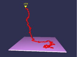
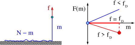
Figure 1: (left) A snapshot from the MC simulation: $N=128,\;h=25.0,\;\epsilon=4.0,;\langle f\rangle=6.126$. (right) Schematic representation of an adsorbed chain of length $N$ which is pulled by the end segment off the surface with force $f$. While $N=m$ monomers lie on the plane, $m$ monomers form the chain tail. The variation of $F(m)$ with $m\in[1,N]$ for super- $f>f_{D}$ and subcritical $f<f_{D}$ forces indicates two different minima (filled circles) of $F$ at $m=N$ and $m=0$ for $f>f_{D}$ and $f<f_{D}$, respectively.

In the following we show that this simplified consideration is indeed confirmed by the more general adsorption model too.

II.2 The Grand Canonical Ensemble approach to chain adsorption

Starting with the conventional (i.e., force-free) case of polymer adsorption, we recall that an adsorbed chain is build up from loops, trains, and a free tail. One can treat statistically these basic structural units by means of the GCE approachPoland ; Bir where the lengths of the buildings blocks are not fixed but may rather fluctuate. The GCE-partition function is then given by an expansion over all possible lengths $N$, see Fig. 2a, which can be considered and summed as a geometric series:

$$\Xi(z)=\sum_{N=0}^{\infty}\>\Xi_{N}\>z^{N}=\frac{V_{0}(z)\>Q(z)}{1-V(z)U(z)}.$$ (1)

In Eq. (1) $z$ is the fugacity and $U(z)$, $V(z)$, and $Q(z)$ denote the GCE partition functions of loops, trains and tails, respectively. The building block adjacent to the tethered chain end is allowed for by $V_{0}(z)=1+V(z)$. The partition function of the loops is defined as $U(z)=\sum_{n=1}^{\infty}\>(\mu_{3}z)^{n}/n^{\alpha}$, where $\mu_{3}$ is the $3d$ connective constant and $\alpha$ is the exponent which governs surface loops statistics. It is well known that for an isolated loop $\alpha=1-\gamma_{11}\approx 1.39$ Vanderzande where $\gamma_{11}=-0.390$. One can proveSBVRAMTV that $\alpha$ changes value, provided the excluded volume interactions between a loop and the rest of the chain are taken into account. The train GCE-partition function reads $V(z)=\sum_{n=1}^{\infty}\>(\mu_{3}wz)^{n}/n^{\lambda}$ with $1-\gamma_{d=2}\approx-0.343$ whereby one assumes that each adsorbed segment gains an additional statistical weight $w=\exp(\epsilon)$. Eventually, the GCE partition function for the chain tail is defined by $Q(z)=1+\sum_{n=1}^{\infty}\>(\mu_{3}z)^{n}/n^{\beta}$. For an isolated tail $\beta=1-\gamma_{1}\approx 0.32$ where $\gamma_{1}=0.680$Vanderzande but again the excluded volume interactions of a tail with the rest of the chain increase the value of $\beta$.

If one knows the GC partition function, Eq. (1), one can find the number of weighted configurations of a polymer chain, containing $N$ segments (i.e., the canonical partition function of such chain), $\Xi_{N}$, by taking the inverse Laplace transform of $\Xi(z)$. Using the generating function method Rudnick , one finds that the main contribution to the coefficient $\Xi_{N}$ at $z^{N}$ is $(z^{*})^{-(N+1)}$ which is provided by the singularity at $z^{*}$ of $\Xi(z)$. There is a simple pole in Eq. (1) at $z=z^{*}$, namely, when $V(z^{*})U(z^{*})=1$. Thus one gets the free energy as $F=k_{B}TN\ln z^{*}$ and the fraction of adsorbed monomers (which defines a convenient order parameter for the phase transition) is $n=-\partial\ln z^{*}/\partial\ln w$. In terms of the so called polylog function, which is defined as $\Phi(\alpha,z)=\sum_{n=1}^{\infty}\>z^{n}/n^{\alpha}$ Erdelyi and exists only for $z\leq 1$, the equation for $z^{*}$ reads

$$\Phi(\alpha,\mu_{3}z^{*})\Phi(\lambda,\mu_{2}wz^{*})=1.$$ (2)

A nontrivial solution for $z^{*}$ in terms of $w$ (or the adsorption energy $\epsilon$) appears at the critical adsorption point (CAP) $w=w_{c}$ - see Fig. 2b - where $\mu_{3}z^{*}=1$. For example, close to the CAP one may expand $\Phi(\alpha,\mu_{3}z^{*})$ with respect to $1-\mu_{3}z^{*}$ so that $w_{c}$ is determined from $\zeta(\alpha)\Phi(1-\gamma_{d=2},\mu_{2}w_{c}/\mu_{3})=1$ where $\zeta(x)$ denotes the Riemann $\zeta$-function.

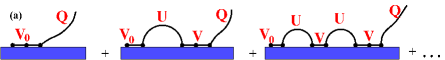
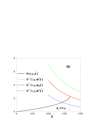
Figure 2: (a) Schematic representation of the series expansion, Eq. (1). (b) The intersection of the polylog functions $\Phi(\alpha,\mu_{3}z^{*})$ and $1/\Phi(\lambda,\mu_{2}wz^{*})$ yields a solution of Eq. (2) for the fugacity $z^{*}$. For adsorption strength $\epsilon<\epsilon_{c}$ the corresponding Boltzmann weight $w^{<}=\exp(\epsilon)$ is insufficient to provide an intersection point (the chain is desorbed) whereas for $\epsilon>\epsilon_{c}$ (for $w^{>}$) a solution for $z^{*}$ exists (the chain is adsorbed). The CAP $\epsilon=\epsilon_{c}$ (i.e. for $w_{c}$) is marked by the first appearance of common point of intersection (full lines) at $z_{c}^{*}=1/\mu_{3}$.

In the vicinity of the CAP the solution attains the form

$$z^{*}(w)\approx[1-A\>(w-w_{c})^{1/(\alpha-1)}]\mu_{3}^{-1}$$ (3)

where $A$ is a constant. Then, for the average fraction of adsorbed monomers one obtains $n\propto(\epsilon-\epsilon_{c})^{1/(\alpha-1)-1}$. A comparison with the well known scaling relationship $n\propto(\epsilon-\epsilon_{c})^{1/\phi-1}$ where $\phi$ is the so called adsorption (or, crossover) exponent Vanderzande suggests that

$$\phi=\alpha-1$$ (4)

This result, derived first by BirshteinBir , is of principal importance. It shows that the exponent $\phi$, which describes polymer adsorption at criticality, is determined by the value of $\alpha$ which governs the polymer loop statistics! If loops are treated as isolated objects, then $\alpha=1-\gamma_{11}\approx 1.39$ so that $\phi=0.39$. In contrast, excluded volume interactions between a loop and the rest of the chain lead to an increase of $\alpha$ and $\phi$, as shown below.

From the expression for $U(z)$, given above, and Eq. (3) we have $P_{\rm loop}\approx(\mu_{3}z^{*})^{l}/l^{1+\phi}\approx\exp[-c_{1}(\epsilon-\epsilon_{c})^{1/\phi}]/l^{1+\phi}$. This is valid only for $\epsilon>\epsilon_{c}$ since a solution for Eq. (2) for subcritical values of the adhesive potential $\epsilon$ does not exist. Nontheless, even in the subcritical region, $\epsilon<\epsilon_{c}$, the monomers occasionally touch the substrate, creating thus single loops at the expense of the tail length. The partition function of such a loop-tail configuration is $Z_{l-t}=\frac{\mu_{3}^{l}}{l^{1+\phi}}\;\frac{\mu_{3}^{N-l}}{(N-l)^{\beta}}$. On the other hand, the partition function of a tail conformation with no loops whatsoever (i.e., of a nonadsorbed tethered chain) is $Z_{t}=\mu_{3}^{N}\;N^{\gamma_{1}-1}$. Thus the probability $P^{<}_{\rm loop}(l)$ to find a loop of length $l$ next to a tail of length $N-l$ can be estimated as $P^{<}_{\rm loop}(l)=\frac{Z_{l-t}}{Z_{t}}\propto\frac{N^{1-\gamma_{1}}}{l^{1+\phi}(N-l)^{\beta}}$ for $\epsilon<\epsilon_{c}$. In the vicinity of the CAP, $\epsilon\approx\epsilon_{c}$, the distribution will be given by an interpolation between the expressions above. Hence, the overall loop distribution becomes

$$P_{\rm loop}(l)=\begin{cases}\frac{1}{l^{1+\phi}}\exp\left[-c_{1}(\epsilon-\epsilon_{c})^{1/\phi}\;l\right],\quad&\quad\epsilon>\epsilon_{c}\\ \frac{A_{1}}{l^{1+\phi}}+\frac{A_{2}N^{1-\gamma_{1}}}{l^{1+\phi}(N-l)^{\beta}},\quad&\quad\epsilon=\epsilon_{c}\\ \frac{N^{1-\gamma_{1}}}{l^{1+\phi}(N-l)^{\beta}}.\quad&\quad\epsilon<\epsilon_{c}\end{cases}$$ (5)

The same reasonings for a tail leads to the distribution

$$P_{\rm tail}(l)=\begin{cases}\frac{1}{l^{\beta}}\exp\left[-c_{1}(\epsilon-\epsilon_{c})^{1/\phi}\;l\right],\quad&\quad\epsilon>\epsilon_{c}\\ \frac{B_{1}}{l^{\beta}}+\frac{B_{2}N^{1-\gamma_{1}}}{l^{\beta}(N-l)^{1+\phi}},\quad&\quad\epsilon=\epsilon_{c}\\ \frac{N^{1-\gamma_{1}}}{l^{\beta}(N-l)^{1+\phi}}.\quad&\quad\epsilon<\epsilon_{c}\end{cases}$$ (6)

In Eqs. (5) - (6) $A_{1},A_{2},B_{1},B_{2}$ are constants. Close to the CAP these distributions are expected to attain a U - shaped form (with two maxima at $l\approx 1$ and $l\approx N$), as predicted for a Gaussian chain by Gorbunov et al. Gorbunov .

For the average loop length $L$ the GCE-partition function for loops yields $L=z\partial U(z)/\partial z|_{z=z^{*}}=\Phi(\alpha-1,\mu_{3}z^{*})/\Phi(\alpha,\mu_{3}z^{*})$. At the CAP, $L$ diverges as $L\propto 1/(\epsilon-\epsilon_{c})^{1/\phi-1}$.

The average tail length $S$ is obtained as $S=z\partial Q(z)/\partial z|_{z=z^{*}}=\Phi(\beta-1,\mu_{3}z^{*})/[1+\Phi(\beta,\mu_{3}z^{*})]$. Again, using the polylog function, one can show that at $\epsilon_{c}$ the average tail length diverges as $S\propto 1/(\epsilon-\epsilon_{c})^{1/\phi}$.

II.3 The interaction of loops and the tail

In the analytical expressions for the PDF of the different building units of a chain, Eqs. (5)-(6) we didn’t elaborate on the numerical values of the exponents $\alpha$ (that is, $\phi$) and $\beta$, taking as an example those for non-interacting polymer chains. However, for a realistic self-avoiding chain one has to allow for the existence of excluded-volume interactions. To this end one may consider the number of configurations of a tethered chain in the vicinity of the CAP as an array of loops which end up with a tail. Using the approach of Kafri et al. Kafri along with Duplantier’s Duplantier graph theory of polymer networks, one may write the partition function $Z$ for a chain with ${\cal N}$ building blocks: ${\cal N}-1$ loops and a tailSBVRAMTV . Consider now a single loop of length $M$ while the length of the rest of the chain is $K$, that is, $M+K=N$. In the limit of $M\gg 1,\;K\gg 1$ (but with $M/K\ll 1$) one can show SBVRAMTV that $Z\sim\mu_{3}^{M}\>M^{\gamma_{\cal N}^{s}-\gamma_{{\cal N}-1}^{s}}\>\>\mu_{3}^{K}\>K^{\gamma_{{\cal N}-1}^{s}-1}$ where the surface exponent $\gamma_{\cal N}^{s}=2+{\cal N}(\nu+1)+\sigma_{1}+\sigma_{1}^{s}$ and $\sigma_{1},\;\sigma_{1}^{s}$ are critical bulk and surface exponents Duplantier . The last result indicates that the effective loop exponent $\alpha$ becomes

$$\alpha=\gamma_{{\cal N}-1}^{s}-\gamma_{\cal N}^{s}=\nu+1$$ (7)

Thus, $\phi=\alpha-1=\nu=0.588$, in agreement with earlier Monte Carlo findings Eisenriegler . One should emphasize, however, that the foregoing derivation is Mean-Field-like ($Z$ appears as a product of loop- and rest-of-the-chain contributions) which overestimates the interactions and increases significantly the value of $\alpha$, serving thus as an upper bound estimate. The value of $\alpha$, therefore, is found to satisfy the inequality $1-\gamma_{11}\leq\alpha\leq 1+\nu$, i.e., depending on loop interactions, $0.39\leq\phi\leq 0.59$.

II.4 Taking the pulling force into account

The GCE approach, described above, can now be employed to tackle the case of self-avoiding polymer chain adsorption in the presence of pulling force. Thus we extend the consideration of Gaussian chains by Gorbunov et al. Skvortsov .

As far as a force $f$ is applied to the end-monomer of a tethered chain, one may choose two possible ways in which the chain detachment from the adsorbing surface can be carried out. One may fix $f$ as an independent control parameter and study the variation of the height $h$ of the end-monomer above the surface plane which corresponds to treatment within the constant force ensemble, herafter referred to as $f$-ensemble. Or, one might fix $h$ and measure the force acting on the end-monomer at a given height, working thus in the constant height ensemble which we call in what follows the $h$-ensemble.

II.4.1 $f$-ensemble

Under pulling force $f$, the tail GCE-partition function $Q(z)$ in Eq. (1) has to be replaced by $\tilde{Q}(z)=1+\sum_{n=1}^{\infty}[(\mu_{3}z)^{n}/n^{\beta}]\>\int d^{3}rP_{n}({\bf r})\exp(fr_{\perp}/T)$ where $P_{n}({\bf r})$ is the end-to-end distance distribution function for a self-avoiding chain DesCloizeaux and $fr_{\perp}$ measures the work, spent to pull the chain end to height $r_{\perp}$ above the adsorbing surface. After some straightforward calculations $\tilde{Q}(z)$ can be written as

$$\tilde{Q}(z)=1+a_{1}\>{\tilde{f}}^{1-\gamma_{1}/\nu}\>\Phi(1-\nu,z\mu_{3}\exp(a_{2}{\tilde{f}}^{1/\nu})$$ (8)

with the dimensionless force ${\tilde{f}}=fa/k_{B}T$. The function $\tilde{Q}(z)$ has a branch point singularity at $z^{\#}=\mu_{3}^{-1}\exp(-a_{2}{\tilde{f}}^{1/\nu})$, i.e., $\tilde{Q}(z)\sim 1/(z^{\#}-z)^{\nu}$. One may, therefore, conclude that the total GCE-partition function $\Xi(z)$ has two singularities on the real axis: the pole $z^{*}$, related to the CAP, and the branch point $z^{\#}$, related to the pulling force. It is known (see, e.g., Sec. 2.4.3. in Rudnick ) that for $N\gg 1$ the main contributions to $\Xi_{N}$ come from the pole and the branch singular points, i.e.,

$$\Xi_{N}\sim C_{1}\>(z^{*})^{-N}+\frac{C_{2}}{\Gamma(\nu)}\>N^{\nu-1}\>(z^{\#})^{-N}$$ (9)

Evidently, for large $N$ only the smallest of these points matters. Note that $z^{*}$ depends on the adsorption energy $\epsilon$ only (through $w=\exp(\epsilon)$) whereas $z^{\#}$ is controlled by the external force ${\tilde{f}}$. Therefore, in terms of the two control parameters, $\epsilon$ and ${\tilde{f}}$, the equation $z^{*}(\epsilon_{D})=z^{\#}({\tilde{f}}_{D})$ defines the critical transition line between the adsorbed phase and the force-induced desorbed phase - Fig. 3. In the following this line will be called detachment line (DL). Below it, $f<f_{D}$, or above, $f>f_{D}$, either $z^{*}$ or $z^{\#}$, respectively, contribute to $\Xi_{N}$. The controll parameters, $\epsilon_{D}$ and ${\tilde{f}}_{D}$, which satisfy this equation, denote detachment energy and detachment force, respectively.

On the DL the system undergoes a first-order phase transition. The DL itself ends for ${\tilde{f}}_{D}\rightarrow 0$ in the CAP, $\epsilon_{c}$, where the transition becomes of second order, as is known for polymer adsorption without pulling. In the vicinity of the CAP the detachment force ${\tilde{f}}_{D}$ is predicted to vanish as ${\tilde{f}}_{D}\sim(\epsilon-\epsilon_{c})^{\nu/\phi}$.

This first order adsorption-desorption phase transition under pulling has a clear dichotomic nature (i.e., it follows an “either - or” scenario): in the thermodynamic limit $N\rightarrow\infty$ there is no phase coexistence! The configurations are divided into adsorbed and desorbed dichotomic classes. Metastable states are completely absent. Moreover, the mean loop length $L$ remains finite upon DL crossing. In contrast, the average tail length $S$ diverges close to the DL. Indeed, at ${\tilde{f}}<{\tilde{f}}_{D}$ the average tail length is given by $S={\tilde{f}}^{1-\gamma_{1}/\nu}\Phi(-\nu,z^{*}(w)/z^{\#}({\tilde{f}}))/[1+a_{1}\Phi(1-\nu,z^{*}(w)/z^{\#}({\tilde{f}}))]$. At the DL, $z^{*}=z^{\#}$, it diverges as $S\propto{\tilde{f}}_{D}/({\tilde{f}}_{D}-{\tilde{f}})$.

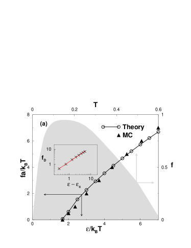
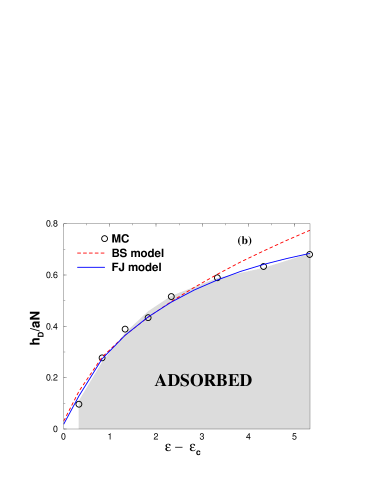
Figure 3: (a) Plot of the critical detachment force $f_{D}=fa/k_{B}T$ against the surface potential $\varepsilon/k_{B}T$. Full and empty symbols denote MC and theoretical results. A double logarithmic plot of $f_{D}$ against $\epsilon-\epsilon_{c}$ with $\epsilon_{c}=1.67$ is shown in the inset, yielding a slope of $0.97\pm 0.02$, in agreement with the prediction $f_{D}\propto(\epsilon-\epsilon_{c})^{\nu/\phi}$. Shaded is shown the same phase diagram, derived by numeric solution of Eq. (2) along with $z^{*}(w)=z^{\#}(\tilde{f})$, which in dimensional $f$ (right axis) against $T$ (top axis) units appears reentrant. (b) The same phase diagram in units of detachment height $h_{D}$ and the distance from the CAP $\epsilon-\epsilon_{c}$. Dashed and solid lines denote theoretical predictions based on the Pincus, or Langevin force vs. elongation relationship while symbols show simulation data.

II.4.2 $h$-ensemble

In the constant height ensemble the way a chain tethered to a surface responds to stretching is described by the tail partition function $\tilde{Q}_{N}$. The partition function of such chain with a fixed distance $h$ of the chain end from the anchoring plane is given

$$\tilde{Q}_{\rm tail}(N,h)=\frac{\mu_{3}^{N}}{N^{\beta}}\>aP_{N}(h)$$ (10)

where again $\beta=1-\gamma_{1}$ and $a$ is the bond length. The deformation of a polymer chain can be described within two models: the bead-spring (BS) model for flexible bonds and the freely jointed chain (FJ) model in which the bonds between monomers are considered rigid. In the BS model one can use for $P_{N}$ the expression Kreer

$$P_{N}(h)=\frac{A}{R_{N}}\>\left(\frac{h}{R_{N}}\right)^{\zeta}\>\exp\left[-D\left(\frac{h}{R_{N}}\right)^{1/(1-\nu)}\right]$$ (11)

where the exponent $\zeta\approx 0.8$, and $A$ is a normalization constant. The free energy of the tethered chain with a fixed distance $h$ takes on the form $F_{\rm tail}(N,h)=-T\ln\tilde{Q}_{\rm tail}(N,h)$. By making use of Eqs. (10) and (11), the expression for the force $f_{N}$, acting on the end-monomer when kept at distance $h$ is given by

$$f_{N}=\frac{\partial}{\partial h}\>F_{\rm tail}(N,h)=\frac{k_{B}T}{R_{N}}\>\left[\frac{D}{1-\nu}\left(\frac{h}{R_{N}}\right)^{\nu/(1-\nu)}-\zeta\left(\frac{R_{N}}{h}\right)\right]$$ (12)

One should note that at $h/R_{N}\gg 1$ we recover the well known Pincus deformation law: $h\propto aN(af_{N}/k_{B}T)^{1/\nu-1}$. In this approximation the (dimensionless) elastic energy reads $U_{\rm el}/k_{B}T=-N(af_{N}/k_{B}T)^{1/\nu}$. In result the corresponding tail free energy is given by

$$\frac{F_{\rm tail}}{k_{B}T}=-N\left(\frac{af_{N}}{T}\right)^{1/\nu}-N\ln\mu_{3}$$ (13)

Eq. (12) indicates that there exists a height $h_{0}=(\zeta(1-\nu)/D)^{1-\nu}R_{N}$ over the surface where the force $f_{N}$ changes sign and becomes negative (that is, the surface repulsion dominates). According to Eq. (12) the force diverges as $f_{N}\propto-k_{B}T/h$ upon further decrease of the distance $h$.

It is well known Grosberg that the Pincus law, Eq. (12), describes the deformation behavior at intermediate force strength, $1/N^{\nu}\ll af_{N}/k_{B}T\leq 1$. Direct Monte Carlo simulation results indicate that, depending on the model, deviations from Pincus law emerge at $h/R_{N}\geq 3$ (bead-spring off-lattice model) Lai , or $h/R_{N}\geq 6$ (Bond Fluctuation Model) Wittkop . In such “overstretched” regime (when the chain is stretched close to its contour length) one should take into account that the chain bonds cannot expand indefinitely. This case could be treated within the simple FJ model Lai where the bond length $a$ is fixed. In this model the force - elongation relationship is given by

$$f_{N}=\frac{k_{B}T}{a}\>{\cal L}^{-1}\left(\frac{h}{aN}\right)$$ (14)

where ${\cal L}^{-1}$ denotes the inverse Langevin function ${\cal L}(x)=\coth(x)-1/x$. The corresponding free energy of the tail for the FJ model reads

$$\frac{F_{\rm tail}}{k_{B}T}=-N{\cal G}\left(\frac{af_{N}}{T}\right)-N\ln\mu_{3}$$ (15)

where we have used the notation ${\cal G}(x)=x{\cal L}(x)=x\coth(x)-1$. One should emphasize that the force $f_{N}$ stays constant in the course of the pulling process (i.e., as long as one monomer, at least, is adsorbed on the surface), thus $f_{N}$ corresponds to a plateau on the elongation curve $f-h$. An adsorbed monomer has a chemical potential, $\mu_{\rm ads}=\ln z^{*}$, which should be equal in equilibrium to the chemical potential of a desorbed monomer in the tail, $\mu_{\rm des}=\partial(F_{\rm tail}/T)/\partial N$. Thus the condition $\mu_{\rm ads}=\mu_{\rm des}$ leads to the following “plateau law” relationship

$$\frac{a\>f_{\rm p}}{k_{B}T}=\begin{cases}\left|\ln[\mu_{3}z^{*}(\epsilon)]\right|^{\nu}&\mbox{, BS model}\\ \\ {\cal G}^{-1}\left(\left|\ln[\mu_{3}z^{*}(\varepsilon)]\right|\right)&\mbox{, FJ model}\end{cases}$$ (16)

with ${\cal G}^{-1}$ being the inverse of the ${\cal G}$ function. Close to the critical point $\epsilon_{c}$ the plateau force $f_{\rm p}\to 0$. Indeed, taking into account that in the vicinity of the critical point $\ln[\mu_{3}z^{*}(\epsilon)]\propto-(\epsilon-\epsilon_{c})^{1/\phi}$ SBVRAMTV and ${\cal G}^{-1}(x)\approx(3x)^{1/2}$ we conclude that $f_{\rm p}\propto(\epsilon-\epsilon_{c})^{\nu/\phi}$ for the BS model and $f_{\rm p}\propto(\epsilon-\epsilon_{c})^{1/2\phi}$ for the FJ model. If the number of tail monomers is denoted by $M$, then the one can write SBVRAMTV $n=-(1/TN)\partial F_{\rm ads}/\partial\epsilon$, where $F_{\rm ads}$ is the free energy of the adsorbed portion of the chain given as $F_{\rm ads}=k_{B}T[N-M(h,\epsilon)]\ln z^{*}(\epsilon)$. From Eq. (16) one can easily obtain $M$ for $h\gg R_{g}$ so that in result one gets

$$n = -\left[1-\frac{M(h,\epsilon)}{N}\right]\frac{\partial\ln z^{*}(\epsilon)}{\partial\epsilon}+\frac{\ln z^{*}(\epsilon)}{N}\>\frac{\partial M(h,\epsilon)}{\partial\epsilon}=$$ (17)

$$= \left|\frac{\partial\ln z^{*}(\epsilon)}{\partial\epsilon}\right|\times\begin{cases}1-\frac{h}{c_{2}aN}\left(\frac{k_{B}T}{af_{\rm p}}\right)^{1/\nu-1}\left[1-{\tilde{c}}_{1}\left(\frac{k_{B}T}{af_{\rm p}}\right)^{1/\nu}|\ln z^{*}|\right]&\mbox{, for BS-model}\\ \\ 1-\frac{h}{c_{3}aN}\left[{\cal L}\left(\frac{af_{\rm p}}{k_{B}T}\right)\right]^{-1}\left[1-\frac{{\cal L}^{\prime}\left(\frac{af_{\rm p}}{k_{B}T}\right)}{{\cal L}\left(\frac{af_{\rm p}}{k_{B}T}\right){\cal G}^{\prime}\left(\frac{af_{\rm p}}{k_{B}T}\right)}\>c_{1}\>|\ln z^{*}|\right]&\mbox{, for FJ-model}\end{cases}$$

where $c_{1},\;c_{2},\;c_{3}$ are constants of the order of unity. The derivatives ${\cal L}^{\prime}(x)=1/x^{2}-1/[\sinh(x)]^{2}$ and ${\cal G}^{\prime}(x)={\cal L}(x)+x{\cal L}^{\prime}(x)=\coth(x)-x/[\sinh(x)]^{2}$ and ${\tilde{c}}_{1}=(1-\nu)c_{1}$.

As one can see from Eq. (17), the order parameter decreases linearly and steadily (no jump!) with growing $h/N$.

II.5 Reentrant phase behavior

Recently, it has been realized Mishra that the DL, force $f_{D}$ versus temperature $T$, when represented in units with dimension, goes (at a relatively low temperature) through a maximum, i.e., the desorption transition shows reentrant behavior! Such behavior has been predicted earlierOrlandini ; Maren ; Kumar1 in a different context, namely, of DNA-unzipping, and also in the coil-hairpin transitionKumar2 .

One can readily see that this result follows directly from our theory. Indeed, the solution of Eq. (2) at large values of $\epsilon$ (that is, at low temperature) can be written as $z^{*}\approx{\rm e}^{-\epsilon}/\mu_{3}$ so that the DL, $z^{*}=z^{\#}$, in terms of dimensionless parameters is monotonous, ${\tilde{f}}_{D}\propto[\epsilon_{D}-\ln(\mu_{3}/\mu_{2})]^{\nu}$. Note, however, that the same DL, if represented in terms of the dimensional control parameters, force $f_{D}$ versus temperature $T_{D}$ (with a fixed energy $\varepsilon_{0}$), shows a nonmonotonic behavior $f_{D}=k_{B}T_{D}[\varepsilon_{0}/T_{D}-\ln(\mu_{3}/\mu_{2})]^{\nu}/a$ - Fig. 3, as found earlier for DNA-unzipping Orlandini . This curve has a maximum at a temperature given by $k_{B}T_{D}^{max}=(1-\nu)\varepsilon_{0}/\ln(\mu_{3}/\mu_{2})$. At very low $T$, however, the expression for $P_{n}({\bf r})$ DesCloizeaux predicts divergent chain deformation Orlandini , i.e., it becomes unphysical. One can readily show that in this case the correct behavior is given by $fa=\varepsilon_{0}+k_{B}T\ln(\mu_{3}/\mu_{2})$.

III Monte Carlo Simulation Model

We use a coarse grained off-lattice bead-spring model MC_Milchev which has proved rather efficient in a number of polymers studies so far. The system consists of a single polymer chain tethered at one end to a flat impenetrable structureless surface - Fig. 1. The surface interaction is described by a square well potential,

$$U_{w}(z)=\begin{cases}\epsilon,&z<r_{c}\\ 0,&z\geq r_{c}\end{cases}$$ (18)

The strength $\epsilon$ is varied from $1.0$ to $7.0$ while the interaction range $r_{c}=0.125$. The effective bonded interaction is described by the FENE (finitely extensible nonlinear elastic) potential:

$$U_{FENE}=-K(1-a)^{2}ln\left[1-\left(\frac{l-a}{l_{max}-a}\right)^{2}\right]$$ (19)

with $K=20,l_{max}=1,a=0.7,l_{min}=0.4$. The nonbonded interactions between monomers are described by the Morse potential:

$$\frac{U_{M}(r)}{\epsilon_{M}}=\exp(-2\alpha(r-r_{min}))-2\exp(-\alpha(r-r_{min}))$$ (20)

with $\alpha=24,\;r_{min}=0.8,\;\epsilon_{M}/k_{B}T=1$. In few cases, needed to clarify the nature of the polymer chain resistance to stretching, we have taken the nonbonded interactions between monomers as purely repulsive by shifting the Morse potential upward by $\epsilon_{M}$ and removing its attractive branch, $V_{M}(r)=0$ for $r\geq r_{min}$.

We employ periodic boundary conditions in the $x-y$ directions and impenetrable walls in the $z$ direction. The lengths of the studied polymer chains are typically $64$, and $128$. The size of the simulation box was chosen appropriately to the chain length, so for example, for a chain length of $128$, the box size was $256\times 256\times 256$ . All simulation results have been averaged over about $2000$ measurements.

The standard Metropolis algorithm was employed to govern the moves with self avoidance automatically incorporated in the potentials. In each Monte Carlo update, a monomer was chosen at random and a random displacement attempted with $\Delta x,\;\Delta y,\;\Delta z$ chosen uniformly from the interval $-0.5\leq\Delta x,\Delta y,\Delta z\leq 0.5$. If the last monomer was displaced in $z$ direction, there was an energy cost of $-f\Delta z$ due to the pulling force. The transition probability for the attempted move was calculated from the change $\Delta U$ of the potential energies before and after the move was performed as $W=exp(-\Delta U/k_{B}T)$. As in a standard Metropolis algorithm, the attempted move was accepted, if $W$ exceeds a random number uniformly distributed in the interval $[0,1]$.

As a rule, the polymer chains have been originally equilibrated in the MC method for a period of about $5\times 10^{5}$ MCS after which typically $500$ measurement runs were performed, each of length $2\times 10^{6}$ MCS. The equilibration period and the length of the run were chosen according to the chain length and the values provided here are for the longest chain length.

IV Comparison of Simulation Data with Theoretical Predictions

We have investigated the force induced desorption of a polymer performing MC simulations in the $f$-ensemble and in the $h$-ensemble. As an order parameter for the desorption transition we use the fraction of monomers $n$ in contact with the sticky surface. Below we present few typical quantities of interest which manifest the good agreement between theoretical predictions and simulation results. Another important point is the observed qualitative difference between the $f-$ and $h-$ensembles in the behavior of some basic properties like the order parameter of the phase transition.

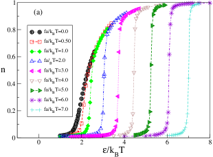
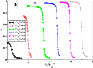
Figure 4: (a) The ’order parameter’, $n$, against the surface potential, $\epsilon$, for various pulling forces $f$. The chain has length $N$=128. (b) Plot of $n$ vs. $f$ for several surface potentials $\epsilon$.

Fig. 4a shows the variation of the order parameter $n$ with changing adhesive potential $\epsilon$ in the $f$-ensemble at fixed pulling force whereas Fig.4b depicts $n$ vs. force $fa/T$ for various $\epsilon$. The abrupt change of the order parameter is in close agreement with our theoretical prediction. Indeed, from Fig. 4 one can readily verify that the polymer detachment transition is of first order.

However, the order parameter variation in the equivalent $h$-ensemble looks very different.

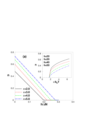
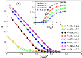
Figure 5: (a) Order parameter $n$ variation with changing height $h/aN$ of the fixed chain-end for polymers of length $N=64,\;128$ and different adsorption strength $\epsilon/k_{B}T$. (b) Variation of $n$ with $\epsilon/k_{B}T$ for different fixed positions of the chain-end $h/aN$.

In Fig. 5a, 5b, we show the change in $n$ with $h$ and in the insets the variation of the fraction of adsorbed segments with adsorption strengths $\epsilon$ for several fixed heights $20\leq h\leq 50$ of the $N=128$ chain. It is evident that, apart from the rounding of the MC data for $n$ at $n\to 0$, which is less pronounced for $N=128$ than for $N=64$, one finds very good agreement between the behavior, predicted by Eq. (17), and the simulation results. Comparing Figs. 4 and 5 one realizes the striking difference between the order parameter behavior in the $f-$ and $h-$ensembles. However, if the height $h$ on the $x$-axis of Fig. 5a is expressed in terms of the corresponding average force $\langle f\rangle$, one recovers again a jump in the order parameter $n$ SKB .

The peculiar nature of the desorption transition under pulling becomes more evident when one plots the PDF of the order parameter in both statistical ensembles. In the presence of a pulling force one observes a remarkable feature of the order parameter probability distribution - Fig. 6a:

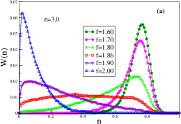
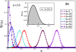
Figure 6: Order parameter distribution of a polymer with $N=128$ and ads adsorption potential $\epsilon=3.0$: (a) in the $f-$ensemble for several values of $f$. The critical detachment force is $f_{D}\approx 1.85\pm 0.01$. (b) in the $h-$ensemble for several fixed heights $h$. The inset displays the distribution $W(n)$ at the critical height of detachment $h_{D}\approx 54.3$.

- an absence of two peaks in the vicinity of the transition force $f_{D}$ although bimodality is customary in first-order phase transition. Immediately at $f_{D}$ the distribution $W(n)$ is flat, indicating huge fluctuations of $n$ so that any value of the number of contacts is equally probable. This lack of bimodality in the $W(n)$ manifests the dichotomic nature of the desorption transition which rules out phase coexistence. In contrast, in the $h-$ensemble, Fig. 6b, one observes an entirely different shape of $W(n)$ with only slight deviations (an appearance of non-zero third moment of the distribution) from Gaussianity in the vicinity of $h_{D}$. The fluctuations of $n$, according to the half-width of $W(n)$, remain finite and almost unchanged for all values of $h$.

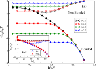
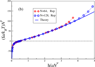
Figure 7: (a) Variation of the two components to the total force, exerted by the chain on the end-monomer which is fixed at (dimensionless) height $h/aN$ for different adsorption potentials $2.0\leq\epsilon/k_{B}T\leq 5.0$ and bonding (FENE) interactions (full symbols) as well as non-bonding (Morse) interactions (empty symbols). In the inset the same is shown for a neutral plane $\epsilon=0.0$ and purely repulsive monomers (triangles) and for the usual Morse potential (circles). (b) Variation of the total applied force $f$ with growing height of the end monomer in terms of Pincus reduced variables, $faN^{\nu}/k_{B}T$ versus $h/aN^{\nu}$, for a polymer with purely repulsive nonbonded forces for $N=64,\;128$.

Eventually, we show in Fig. 7a the typical plateau observed in the average pulling force when the polymer detachment is effected in the $h$-ensemble. Within a large interval of height variation the mean force, exerted on the end monomer, remains constant as observed in laboratory experiments. A rapid growth in the magnitude of this force sets in after the plateau, as soon as the bonds rather that the confortmation of the polymer are stretched upon further elongation. The stronger the adsorption, $\epsilon$, the larger the force $f_{D}$ required to remove the chain from the substrate.

In addition to the force due to bonded interactions, however, one can see a small contribution from the non-bonded (attractive) interactions between the chain segments. This contribution is not allowed for by the GCE theory and, therefore, a test with the theoretical preedictions should exclude it. If the attractive branch of the Morse potential is removed, leaving the self-excluded repulsive branch only, this contribution almost vanishes - Fig. 7a (inset).

The elongation vs. force relationship, predicted by Eq. (12), is tested in Fig. 7b for chains in which only non-bonded repulsion between segments exists. For small and intermediate extensions $h$ where $f$ is not too large the agreement with Pincus law is found to be perfect although it deteriorates for larger $f$, as expected. In the latter region one may show that a very good agreement between theory and computer experiment is provided by the FJ model - Eq. (14). From Fig. 7b one can also see that $f$ goes through zero before the height has become zero, that is, no force is felt when the chain end is kept at this particular height. Further decrease of $h$ leads to change of sign of $f$, indicating the entropic repulsion of the polymer coil from the solid surface.

V Summary

In conclusion, we have shown that a full description of the force-induced desorption of a self-avoiding polymer chain can be achieved by means of the GCE approach, yielding the average size and probability distribution functions of all basic structural units of partially adsorbed polymer as well as their variation with changing force or strength of adhesion. All these predictions appear in good agreement with our MC simulation results.

The polymer detachment transition under pulling is found to be of first order whereby due to its dichotomic nature phase coexistence is impossible. This absence of binodal states makes the polymer desorption under pulling a rather unusual in comparison to conventional first-order phase transformation.

The critical line of desorption, while growing steadily when plotted in dimensionless units of detachment force against surface potential, appears “reentrant“ in absolute units of force against temperature. Thus, at very low temperature the polymer is expected to be desorbed, with the growing $T$ it may adsorb, and at even higher temperature - desorb again from the surface.

One finds that the crossover exponent, $\phi$, governing polymer adsorption at criticality, whose exact value has been controversial for a long time, depends essentially on interactions between different loops so that $\phi$ may only vary within the limits $0.39\leq\phi\leq 0.59$.

A point of more general importance for the statistical mechanics in general and theory of phase transitions in particular is the issue of ensemble equivalence. The latter implies an identity of the equation of state, regardless of which statistical ensemble has been employed, whereas the fluctuations within the different ensembles may be entirely differentSKB . For finite polymer lengths, however, differences in the equation of state may also be visible. As far as in practice one deals with finite polymer chains in laboratory experiments, this difference is expected to be clearly manifested in cases of practical concern.

Acknowledgments We are indebted to A. Skvortsov, L. Klushin, J.-U. Sommer, and K. Binder for useful discussions during the preparation of this work. A. Milchev thanks the Max-Planck Institute for Polymer Research in Mainz, Germany, for hospitality during his visit in the institute. A. Milchev and V. Rostiashvili acknowledge support from the Deutsche Forschungsgemeinschaft (DFG), grant No. SFB 625/B4.

References

- (1) M. Rief, F. Oseterfeld, B. Heymann, H. E. Gaub: Science, 275, 1295 (1997).
- (2) S. B. Smith, Y. Cui, C. Bustamante: Science, 271, 795 (1996).
- (3) T. Strick, J.-F. Allemand, V. Croquette, D. Bensimon: Phys. Today, 54, 46(2001).
- (4) F. Celestini, T. Frish, X. Oycharcabal: Phys. Rev. 70, 012801(2008).
- (5) E. L. Florin, V. T. Moy, H. E. Gaub: Science, 264, 415(1994).
- (6) A. Serr, R. R. Netz: Europhys. Lett. 73, 292(2006).
- (7) B. J. Haupt,et al. Langmuir, 15, 3868 (1999).
- (8) A. M. Skvortsov, et al., Polymer Sci. A (Moscow) (2009).
- (9) Y. Kafri, et al. Eur. Phys. J. B 27, 135 (2002).
- (10) D. Poland, H.A. Scheraga, J. Chem. Phys. 45, 1456 (1966).
- (11) T. M. Birshtein, Macromolecules, 12, 715(1979); ibid. 16, 45(1983).
- (12) B. Duplantier, J. Stat. Phys. 54, 581 (1989).
- (13) C. Vanderzande, Lattice Model of Polymers, Cambridge University Press, Cambridge, 1998.
- (14) S. Bhattacharya et al., Macromolecules (in press)
- (15) J.A. Rudnick, G.D. Gaspari, Elements of the random walk, Cambridge University Press, Cambridge, 2004.
- (16) A. Erdélyi, Higher transcendental functions, McGraw Hill, v.1, N.Y., 1953.
- (17) A. A. Gorbunov, et al. J. Chem. Phys. 114, 5366 (2001).
- (18) E. Eisenriegler, K. Kremer, K. Binder, J. Chem. Phys. 77, 6296 (1982).
- (19) A.A. Gorbunov, A.M. Skvortsov, J. Chem. Phys. 98, 5961 (1993).
- (20) J. des Cloizeaux, G. Jannink, Polymers in Solution, Clarendon Press, Oxford, 1990.
- (21) T. Kreer, S. Metzger, M. M’́uller, and K. Binder, J. Chem. Phys. 120, 4012 (2004).
- (22) A.Yu. Grosberg, A.R. Khokhlov,Statistical Physics of Macromolecules (AIP, New York, 1994).
- (23) Y.-J. Sheng, P.-Y. Lai, Phys. Rev. E 56, 1900 (1997).
- (24) M. Wittkop, J.-U. Sommer, S. Kreitmeier, D. Göritz, Phys. Rev. E 49, 5472 (1994).
- (25) P.K. Mishra,et al. Europhys. Lett. 69, 102 (2005).
- (26) E. Orlandini et al. J. Phys. A, 34, L751 (2001).
- (27) D. Marenduzzo, A. Trovato, and A. Maritan, Phys. Rev. E, 64, 031901 (2001).
- (28) S. Kumar and D. Giri, J. Chem. Phys. 125, 044905 (2006).
- (29) S. Kumar, D. Giri, and Y. Singh, Europhys. Lett. 70, 15 (2005).
- (30) K. Binder and A. Milchev, J. Computer-Aided Material Design, 9, 33(2002).