On the $k$-gamma $q$-distribution

Abstract

We provide combinatorial as well as probabilistic interpretations for the $q$-analogue of the Pochhammer $k$-symbol introduced by Díaz and Teruel. We introduce $q$-analogues of the Mellin transform in order to study the $q$-analogue of the $k$-gamma distribution.

1 Introduction

There is a general strategy for building bridges between combinatorics and measure theory which we describe. Let $d\mu$ be a measure on a interval $I\subseteq[0,\infty)\subseteq\mathbb{R}$. We say that $d\mu$ is a combinatorial measure if for each $n\in\mathbb{N}$ the $n$-th moment of $d\mu$ is a non-negative integer. Equivalently, let $M_{d\mu}$ be the Mellin transform of $d\mu$ given by

$$M_{d\mu}(t)=\int_{I}x^{t-1}d\mu.$$

Then $d\mu$ is a combinatorial measure if and only if $M_{d\mu}(n)\in\mathbb{N}$ for $n\in\mathbb{N}_{+}.$

Let $cmeas$ be the set of combinatorial measures, and consider the map $m:cmeas\rightarrow\mathbb{N}^{\mathbb{N}}$ that sends a combinatorial measure into its moment’s sequence $(m_{0},...,m_{n},...).$ Recall [14] that a sequence of finite sets $(s_{0},...,s_{n},...)$ provides a combinatorial interpretation for a sequence of integers $(m_{0},...,m_{n},...)$ if it is such that $|s_{n}|=m_{n}.$ By analogy we say that the sequence of finite sets $(s_{0},...,s_{n},...)$ provides a combinatorial interpretation for a measure $d\mu$ if for each $n\in\mathbb{N}$ the following identity holds:

$$|s_{n}|=\int_{I}x^{n}d\mu.$$

In this work we consider the reciprocal problem: given $m=(m_{0},...,m_{n},...)\in\mathbb{N}$ find a combinatorial interpretation for it, and furthermore find a combinatorial measure $d\mu$ such that its sequence of moments is $m$. Our main goal is to establish an instance of the correspondence combinatorics/measure theory described above within the context of $q$-calculus. Namely, we are going to study the combinatorial and the measure theoretic interpretations for the $k$-increasing factorial $q$-numbers $[1]_{n,k}=[1]_{q}[1+k]_{q}[1+2k]_{q}.\ .\ .[1+(n-1)k]_{q}\in\mathbb{N}[q]^{\mathbb{N}}$ which are obtained as an instance of the $q$-analogue of the Pochhammer $k$-symbol given by

$$[t]_{n,k}=[t]_{q}[t+k]_{q}[t+2k]_{q}.\ .\ .[t+(n-1)k]_{q}=\prod_{j=0}^{n-1}[t+jk]_{q}$$

where $[t]_{q}=\frac{1-q^{t}}{1-q}$ is the $q$-analogue of $t$. The search for the combinatorial and measure theoretic interpretation for the $k$-increasing factorial $q$-numbers must be made within the context of $q$-calculus; this means that we have to broaden our techniques in order to include $q$-combinatorial interpretations, and the $q$-analogues for the Lebesgue’s measure and the Mellin’s transform.

2 The $k$-gamma measure

Perhaps the best known example of the relation combinatorics/measure theory discussed in the introduction comes from the factorial numbers $n!$ which count, respectively, the number of elements of $S_{n}$, the group of permutations of a set with $n$ elements. The Mellin transform of the measure $e^{-x}dx$ is the classical gamma function given for $t>0$ by

$$\Gamma(t)=\int_{0}^{\infty}x^{t-1}e^{-x}dx.$$

The moments of the measure $e^{-x}dx$ are precisely the factorial numbers, indeed we have that

$$|S_{n}|=n!=\Gamma(n+1)=\int_{0}^{\infty}x^{n}e^{-x}dx.$$

Notice that $n!=(1)_{n},$ where the Pochhammer symbol $(t)_{n}$ is given by

$$(t)_{n}=t(t+1)(t+2).\ .\ .(t+(n-1)).$$

As a second example [5] consider the combinatorial and measure theoretical interpretations for the $k$-increasing factorial numbers $(1)_{n,k}=(1+k)(1+2k).\ .\ .(1+(n-1)k),$ which arise as an instance of the Pochhammer $k$-symbol given by

$$(t)_{n,k}=t(t+k)(t+2k).\ .\ .(t+(n-1)k)=\prod_{j=0}^{n-1}(t+jk).$$

The combinatorics of the Pochhammer $k$-symbol has attracted considerable attention in the literature, from the work of Gessel and Stanley [10] up to the quite recent works [2, 12]. Assume $t$ is a non-negative integer and let $\mathrm{T}_{n,k}^{t}$ be the set of isomorphisms classes of planar rooted trees $T$ such that: 1) The set of internal vertices, i.e. vertices with one outgoing edge and at least one incoming edge, of $T$ is $\{1,2,....,n\}$; 2) $T$ has a unique vertex with no outgoing edges called the root; $T$ has a set $L(T)$ of vertices called leaves, the leaves have no incoming edges; 3) The valence of each internal vertex of $T$ is $k+2;$ 4) The valence of the root is $t$; 5) If the internal vertex $i$ is on the path from the internal vertex $j$ to the root, then $i<j.$

Note that the set of leaves $L(T)$ comes with a natural order, and thus we can assign a number between $1$ to $|L(T)|$ to each leave. Figure 1 shows an example of a graph in $\mathrm{T}_{4,2}^{2}$.

One can show by induction that $(t)_{n,k}=|\mathrm{T}_{n,k}^{t}|.$

Figure 1: Example of a tree in $\mathrm{T}_{4,2}^{2}$.

The Mellin transform of the measure $e^{\frac{-x^{k}}{k}}dx$ is the $k$-gamma function $\Gamma_{k}$ given for $t>0$ by

$$\Gamma_{k}(t)=\int_{0}^{\infty}x^{t-1}e^{-\frac{x^{k}}{k}}dx.$$

The $k$-gamma function $\Gamma_{k}:(0,\infty)\longrightarrow\mathbb{R}$ is univocally determined [5] by the following properties: $\Gamma_{k}(t+k)=t\Gamma_{k}(t)$ for $t\in\mathbb{R^{+}};$ $\Gamma_{k}(k)=1;$ $\Gamma_{k}$ is logarithmically convex. See [11, 13] for further properties of the $k$-gamma function.

The $k$-increasing factorial numbers appear as moments of the $\Gamma_{k}$ function as follows:

$$|\mathrm{T}_{n,k}^{1}|=(1)_{n,k}=\Gamma_{k}(1+nk)=\frac{1}{\Gamma_{k}(1)}\int_{0}^{\infty}x^{nk}e^{\frac{-x^{k}}{k}}dx=\frac{k^{\frac{k-1}{k}}}{\Gamma(\frac{1}{k})}\int_{0}^{\infty}x^{nk}e^{\frac{-x^{k}}{k}}dx.$$

Indeed the following more general identity holds:

$$|\mathrm{T}_{n,k}^{t}|=(t)_{n,k}=\frac{\Gamma_{k}(t+nk)}{\Gamma_{k}(t)}=\frac{1}{\Gamma_{k}(t)}\int_{0}^{\infty}x^{t+nk-1}e^{\frac{-x^{k}}{k}}dx.$$

3 Review of $q$-calculus

In this section we introduce some useful basic definitions [1, 3, 9]. We begin introducing the $q$-derivative and the Jackson $q$-integral. Let $\mathrm{Map}(\mathbb{R},\mathbb{R})$ be the real vector space of functions from $\mathbb{R}$ to $\mathbb{R}$. Fix a real number $0\leq q<1,$ the $q$-derivative is the linear operator

$$\partial_{q}:\mathrm{Map}(\mathbb{R},\mathbb{R})\rightarrow\mathrm{Map}(\mathbb{R}\setminus\{0\},\mathbb{R})\ \ \ \ \ \mbox{given by}$$

$$\partial_{q}f(x)=\frac{f(qx)-f(x)}{(q-1)x}.\ \ \ \ \mbox{For example we have that}\ \ \partial_{0}f(x)=\frac{f(x)-f(0)}{x}.$$

Notice that $\partial_{q}f$ is not a priori well-defined at $x=0$. Nevertheless, it is often the case that $\partial_{q}f$ can be extended by continuity over the whole real line, e.g. when $f$ is a polynomial function.

For $0\leq a<b\leq+\infty$ the Jackson $q$-integral from $a$ to $b$ of $f\in\mathrm{Map}(\mathbb{R},\mathbb{R})$ is given by

$$\int_{a}^{b}f(x)d_{q}x=(1-q)b\sum_{n=0}^{\infty}q^{n}f(q^{n}b)-(1-q)a\sum_{n=0}^{\infty}q^{n}f(q^{n}a).$$

For example we have that

$$\int_{a}^{b}f(x)d_{0}x=bf(b)-af(a).$$

Set $I_{q}f(x)=f(qx).$ The following properties hold for $f,g\in\mathrm{Map}(\mathbb{R},\mathbb{R}):$

$$\partial_{q}(fg) = \partial_{q}fg+I_{q}f\partial_{q}g$$

$$\partial_{q}(f(ax^{b})) = a[b]_{q}x^{b-1}\partial_{q^{b}}f(ax^{b})$$

$$f(b)g(b)-f(a)g(a) = \int_{a}^{b}\partial_{q}fgd_{q}x+\int_{a}^{b}I_{q}g\partial_{q}fd_{q}x,$$

For $0<q<1$, $x,y\in\mathbb{R}$, $n\in\mathbb{N}_{+}$, and $t\in\mathbb{R}$ we set

$$(x+y)_{q^{k}}^{n}=\prod_{j=0}^{n-1}(x+q^{jk}y),\ \ \ (x+y)_{q^{k}}^{\infty}=\prod_{j=0}^{\infty}(x+q^{jk}y)\mbox{\ \ \ and \ \ \ }(1+x)_{q^{k}}^{t}=\frac{(1+x)_{q^{k}}^{\infty}}{(1+q^{kt}x)_{q^{k}}^{\infty}}.$$

4 $q$-Analogue of the $k$-gamma function

We proceed to study the $q$-analogue of the $k$-increasing factorial numbers

$$[1]_{n,k}=[1]_{q}[1+k]_{q}[1+2k]_{q}.\ .\ .[1+(n-1)k]_{q}$$

which are an instance of the $q$-analogue of the Pochhammer $k$-symbol $[t]_{n,k}$ given for $t\in\mathbb{R}$ by

$$[t]_{n,k}=[t]_{q}[t+k]_{q}[t+2k]_{q}.\ .\ .[t+(n-1)k]_{q}=\prod_{j=0}^{n-1}[t+jk]_{q}.$$

The motivation behind our definition of the $q$-analogue of the $k$-gamma function comes from the work of De Sole and Kac [4], where they introduced a $q$-deformation of the gamma function given by the $q$-integral:

$$\Gamma_{q}(t)=\int_{0}^{\frac{1}{1-q}}x^{t-1}E_{q}^{-qx}d_{q}x,$$

where the $q$-analogue $E_{q}^{x}$ of the exponential function is given by

$$E_{q}^{x}=\sum_{n=0}^{\infty}q^{\frac{n(n-1)}{2}}\frac{x^{n}}{[n]_{q}!}.$$

For example we have that $E_{0}^{x}=1+x,$ $E_{0}^{-0x}=1$, and therefore $\Gamma_{0}(t)=1.$

We define the $q$-analogue of the $k$-gamma function $\Gamma_{q,k}$ by demanding that it satisfies the $q$-analogues of the properties of the $\Gamma_{k}$ function. Thus $\Gamma_{q,k}$ is such that $\Gamma_{q,k}(t+k)=[t]_{q}\Gamma_{q,k}(t)$ and $\Gamma_{q,k}(k)=1.$ Several applications of the former property show that

$$\Gamma_{q,k}(nk)=\prod_{j=1}^{n-1}[jk]_{q}=\prod_{j=1}^{n-1}\frac{(1-q^{jk})}{{(1-q)}}=\frac{(1-q^{k})_{q^{k}}^{n-1}}{(1-q)^{n-1}}.$$

After a change of variables the function $\Gamma_{q,k}$ may be written as follows:

$$\Gamma_{q,k}(t)=\frac{{(1-q^{k})_{q^{k}}^{{\frac{t}{k}}-1}}}{{(1-q)^{\frac{t}{k}-1}}}.\ \ \ \ \mbox{For example we have that}\ \ \Gamma_{0,k}(t)=1.$$

The previous formula implies an infinite product expression for $\Gamma_{q,k}$ given by

$$\Gamma_{q,k}(t)=\frac{(1-q)^{1-\frac{t}{k}}(1-q^{k})_{q^{k}}^{\infty}}{(1-q^{t})_{q^{k}}^{\infty}},$$

and also the following result.

Lemma 1.

The $q,k$-gamma function $\Gamma_{q,k}$ and the $q^{k}$-gamma function $\Gamma_{q^{k}}$ are related by the identity $\ \ \Gamma_{q,k}(t)=[k]_{q}^{\frac{t}{k}-1}\Gamma_{q^{k}}(\frac{t}{k}).$

The following result [8] provides an integral representation for $\Gamma_{q,k}$.

Proposition 2.

$$\Gamma_{q,k}(t)=\int_{0}^{\frac{[k]_{q}^{\frac{1}{k}}}{(1-q^{k})^{\frac{1}{k}}}}x^{t-1}E_{q^{k}}^{-\frac{q^{k}x^{k}}{[k]_{q}}}d_{q}x.$$

This integral representation for $\Gamma_{q,k}$ may be regarded as a $q$-analogue of the Mellin transform, therefore one is entitled to consider the $q$-measure

$$E_{q^{k}}^{-\frac{q^{k}x^{k}}{[k]_{q}}}d_{q}x\ \ \ \mbox{defined on the interval}\ \ \ \big{[}0,\frac{[k]_{q}^{\frac{1}{k}}}{(1-q^{k})^{\frac{1}{k}}}\big{]}$$

as the inverse Mellin $q$-transform of the $\Gamma_{q,k}$ function. Figure 2 shows the graph of $E_{q^{k}}^{-\frac{q^{k}x^{k}}{[k]_{q}}}$ for $q=0.6$ and $1\leq k\leq 5$.

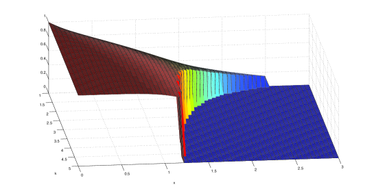
Figure 2: Display of $E_{q^{k}}^{-\frac{q^{k}x^{k}}{[k]_{q}}}$ for $q=0.6$ and $1\leq k\leq 5$.

One can check that for $0\leq x\leq\frac{[k]_{q}^{\frac{1}{k}}}{(1-q^{k})^{\frac{1}{k}}}$ the function $E_{q^{k}}^{-\frac{q^{k}x^{k}}{[k]_{q}}}$ is given by

$$E_{q^{k}}^{-\frac{q^{k}x^{k}}{[k]_{q}}}=\sum_{n=0}^{\infty}\frac{(-1)^{n}q^{\frac{kn(n+1)}{2}}x^{kn}}{[k]_{q}^{n}[n]_{q^{k}}!}.$$

Theorem 3.

The function $\Gamma_{q,k}$ is given by

$$\Gamma_{q,k}(t)=(1-q)^{1-\frac{t}{k}}\sum_{n=0}^{\infty}\frac{q^{\frac{kn(n+1)}{2}}}{(1-q^{kn+t})(q^{k}-1)^{n}[n]_{q^{k}}!}.$$

Proof.

From Theorem 7 below we know that

$$\int_{0}^{x}s^{t-1}E_{q^{k}}^{-\frac{q^{k}s^{k}}{[k]_{q}}}d_{q}s=(1-q)x^{t}\sum_{n=0}^{\infty}\frac{(-1)^{n}q^{\frac{kn(n+1)}{2}}x^{kn}}{(1-q^{kn+t})[k]_{q}^{n}[n]_{q^{k}}!}.$$

The desired result follows taking $x=\frac{[k]_{q}^{\frac{1}{k}}}{(1-q^{k})^{\frac{1}{k}}}$. ∎

Corollary 4.

$$(1-q^{k})_{q^{k}}^{\frac{t}{k}}=\sum_{n=0}^{\infty}\frac{q^{\frac{kn(n+1)}{2}}}{(1-q^{kn+t})(q^{k}-1)^{n}[n]_{q^{k}}!}.$$

Proof.

Follows from Theorem 3 and the identity $\Gamma_{q,k}(t)=\frac{{(1-q^{k})_{q^{k}}^{{\frac{t}{k}}-1}}}{{(1-q)^{\frac{t}{k}-1}}}.$ ∎

By definition the cumulative distribution function associated with the measure

$$E_{q^{k}}^{-\frac{q^{k}x^{k}}{[k]_{q}}}d_{q}x\ \ \ \ \mbox{is given for}\ \ \ 0\leq x\leq\frac{[k]_{q}^{\frac{1}{k}}}{(1-q^{k})^{\frac{1}{k}}}\ \ \ \ \mbox{by}\ \ \ \int_{0}^{x}E_{q^{k}}^{-\frac{q^{k}s^{k}}{[k]_{q}}}d_{q}s.$$

Proposition 5.

$$\int_{0}^{x}E_{q^{k}}^{-\frac{q^{k}s^{k}}{[k]_{q}}}d_{q}s=(1-q)x\sum_{n=0}^{\infty}\frac{(-1)^{n}q^{\frac{kn(n+1)}{2}}x^{kn+1}}{(1-q^{kn+1})[k]_{q}^{n}[n]_{q^{k}}!}.$$

Proof.

The result follows from Theorem 7 below taking $t=1.$

∎

5 Combinatorial interpretation of the Pochhammer $q,k$-symbol

Just as in combinatorics one studies the cardinality of finite sets, in $q$-combinatorics one studies the cardinality of $q$-weighted finite sets, i.e. pairs $(x,\omega)$ where $x$ is a finite set and the $q$-weight is an arbitrary map $\omega:x\rightarrow\mathbb{N}[q]$ from $x$ to $\mathbb{N}[q]$ the algebra of polynomials in $q$ with non-negative integer coefficients. The cardinality of the pair $(x,\omega)$ is by definition given by

$$|x,\omega|=\sum_{i\in x}\omega(i)\in\mathbb{N}[q].$$

To provide a $q$-combinatorial interpretation for the Pochhammer $k$-symbol $[t]_{n,k}$ we let again $t$ be a positive integer and consider the set $\mathrm{T}_{n,k}^{t}$ of planar rooted trees introduced above. Next we define a $q$-weight $\omega$ on $\mathrm{T}_{n,k}^{t}$. The construction of $\omega$ is based on the following elementary facts:

Figure 3: Display of the tree $r_{3}$ and a tree $c_{i}$ with $5$ leaves.

1) Let $r_{t}$ be the rooted tree with $t$ leaves and no internal vertices. See Figure 3.

2) For $1\leq i\leq n$, let $c_{i}$ be the rooted tree with $i$ as its unique internal vertex and $k+1$ leaves. See Figure 3.

3) If $T$ is a planar rooted tree and $l$ is a number between $1$ and $|L(T)|$, then there is a well-defined rooted planar tree $T\circ_{l}c_{i}$ obtained by gluing the root of $c_{i}$ with the leave $l$ of $T$ to form a new edge.

4) Clearly each tree $T\in\mathrm{T}_{n,k}^{t}$ can be written in a unique way as

$$T=(...((r_{t}\circ_{l_{1}}c_{1})\circ_{l_{2}}c_{2})...)\circ_{l_{n}}c_{n}.$$

5) The weight $\omega(T)$ of a tree $T$ written in the form above is given by

$$\omega(T)=\prod_{i=1}^{n-1}q^{l_{i}-1}\in\mathbb{N}[q].$$

For the tree $T$ from Figure 1 we have that

$$T=(((r_{2}\circ_{1}c_{1})\circ_{3}c_{2})\circ_{6}c_{3})\circ_{7}c_{4}\ \ \mbox{ and }\ \ \omega(T)=q^{0}q^{2}q^{5}q^{6}=q^{13}.$$

Theorem 6.

$$[t]_{n,k}=|\mathrm{T}_{n,k}^{t},\omega|.$$

Proof.

The proof goes by induction on $n$. We have the following chain of identities

$$|\mathrm{T}_{n+1,k}^{t},\omega|=\sum_{T\in\mathrm{T}_{n+1,k}^{t}}\omega(T)=\sum_{S\in\mathrm{T}_{n,k}^{t}}\sum_{l\in L(S)}\omega(S\circ_{l}c_{n+1})=\sum_{S\in\mathrm{T}_{n,k}^{t}}\sum_{l=1}^{t+kn}\omega(S)q^{l-1}=$$

$$=\left(\sum_{S\in\mathrm{T}_{n,k}^{t}}\omega(S)\right)\left(\sum_{l=1}^{t+nk}q^{l-1}\right)=|\mathrm{T}_{n+1,k}^{t},\omega|[t+nk]_{q}=[t]_{n,k}[t+nk]_{q}=[t]_{n+1,k}.$$

In the computation above we used two main facts: 1) Each tree $\mathrm{T}_{n,k}^{t}$ has exactly $t+nk$ leaves; 2) Each tree $T\in\mathrm{T}_{n+1,k}^{t}$ can be written in a unique way as $T=S\circ_{l}c_{n+1}$ where $S\in\mathrm{T}_{n,k}^{t}$, $l$ is a leaf of $S$, and $c_{n+1}$ is the rooted tree with $k+1$ leaves and $n+1$ as its unique internal vertex.

∎

6 $k$-Gamma $q$-distribution

We are ready to define the $k$-gamma $q$-distribution. From the identity

$$\Gamma_{q,k}(t)=\int_{0}^{\frac{[k]_{q}^{\frac{1}{k}}}{(1-q^{k})^{\frac{1}{k}}}}x^{t-1}E_{q^{k}}^{-\frac{q^{k}x^{k}}{[k]_{q}}}d_{q}x$$

we see that the function

$$x^{t-1}\frac{E_{q^{k}}^{-\frac{q^{k}x^{k}}{[k]_{q}}}}{\Gamma_{q,k}(t)}$$

defines a $q$-density on the interval $[0,\frac{[k]_{q}^{\frac{1}{k}}}{(1-q^{k})^{\frac{1}{k}}}]$, in the sense that it is a non-negative function whose $q$-integral is equal to one. Consider the case $t=1$ an $k=3$. Figure 4 shows the graph of $\frac{E_{q^{3}}^{-\frac{q^{3}x^{3}}{[3]_{q}}}}{\Gamma_{q,3}(1)}$ for $q\in[0,1)$.

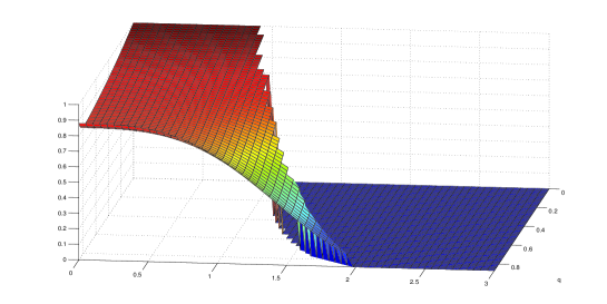
Figure 4: Display of $\frac{E_{q^{3}}^{-\frac{q^{3}x^{3}}{[3]_{q}}}}{\Gamma_{q,3}(1)}$ for $q\in[0,1)$.

Theorem 7.

The cumulative distribution of the $k$-gamma $q$-density is given by

$$\frac{1}{\Gamma_{q,k}(t)}\int_{0}^{x}s^{t-1}E_{q^{k}}^{-\frac{q^{k}s^{k}}{[k]_{q}}}d_{q}s=\frac{(1-q)x^{t}}{\Gamma_{q,k}(t)}\sum_{n=0}^{\infty}\frac{(-1)^{n}q^{\frac{kn(n+1)}{2}}x^{kn}}{[k]_{q}^{n}[n]_{q^{k}}!(1-q^{kn+t})}.$$

Proof.

$$\frac{1}{\Gamma_{q,k}(t)}\int_{0}^{x}s^{t-1}E_{q^{k}}^{-\frac{q^{k}s^{k}}{[k]_{q}}}d_{q}s = \frac{(1-q)x}{\Gamma_{q,k}(t)}\sum_{m=0}^{\infty}q^{m}\sum_{n=0}^{\infty}\frac{(-1)^{n}q^{\frac{kn(n+1)}{2}}(q^{m}x)^{kn+t-1}}{[k]_{q}^{n}[n]_{q^{k}}!}$$

$$= \frac{1-q}{\Gamma_{q,k}(t)}\sum_{n=0}^{\infty}\frac{(-1)^{n}q^{\frac{kn(n+1)}{2}}x^{kn+t}}{[k]_{q}^{n}[n]_{q^{k}}!}\sum_{m=0}^{\infty}q^{m(kn+t)}$$

$$= \frac{1-q}{\Gamma_{q,k}(t)}\sum_{n=0}^{\infty}\frac{(-1)^{n}q^{\frac{kn(n+1)}{2}}x^{kn+t}}{[k]_{q}^{n}[n]_{q^{k}}!(1-q^{kn+t})}$$

∎

Consider the case $t=1$ an $k=3$.Figure 5 shows the cumulative distribution associated to the $q$-density $\frac{E_{q^{3}}^{-\frac{q^{3}x^{3}}{[3]_{q}}}}{\Gamma_{q,3}(1)}$ for $q\in[0,1)$.

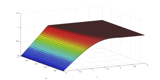
Figure 5: Cumulative distribution of the $q$-density $\frac{E_{q^{3}}^{-\frac{q^{3}x^{3}}{[3]_{q}}}}{\Gamma_{q,3}(1)}$ for $q\in[0,1)$.

The previous considerations imply our next result which establishes an example of the link between $q$-combinatorics and $q$-measure theory promised in the introduction.

Theorem 8.

The $k$-increasing factorial $q$-numbers appear as moments of the $\Gamma_{q,k}$ function as follows:

$$|\mathrm{T}_{n,k}^{1},\omega|=[1]_{n,k}=\Gamma_{q,k}(1+nk)=\frac{1}{\Gamma_{q,k}(1)}\int_{0}^{\frac{[k]_{q}^{\frac{1}{k}}}{(1-q^{k})^{\frac{1}{k}}}}x^{nk}E_{q^{k}}^{-\frac{q^{k}x^{k}}{[k]_{q}}}d_{q}x.$$

Indeed the following more general identity also holds:

$$|\mathrm{T}_{n,k}^{t},\omega|=[t]_{n,k}=\frac{\Gamma_{q,k}(t+nk)}{\Gamma_{q,k}(t)}=\frac{1}{\Gamma_{q,k}(t)}\int_{0}^{\frac{[k]_{q}^{\frac{1}{k}}}{(1-q^{k})^{\frac{1}{k}}}}x^{t+nk-1}E_{q^{k}}^{-\frac{q^{k}x^{k}}{[k]_{q}}}d_{q}x.$$

7 $k$-Beta $q$-distribution

Recall that the classical beta function is given for $s,t>0$ by

$$B(t,s)=\frac{\Gamma(t)\Gamma(s)}{\Gamma(t+s)}=\int_{0}^{1}x^{t-1}(1-x)^{s-1}dx.$$

The $q$-analogue of the $k$-beta function is correspondingly defined by

$$B_{q,k}(t,s)=\frac{\Gamma_{q,k}(t)\Gamma_{q,k}(s)}{\Gamma_{q,k}(t+s)}=\frac{(1-q)(1-q^{k})_{q^{k}}^{\frac{s}{k}-1}}{(1-q^{t})_{q^{k}}^{\frac{s}{k}}}.$$

Notice that $B_{0,k}(t,s)=1$. One can show [8] that the function $B_{q,k}$ has the following integral representation

$$B_{q,k}(t,s)=[k]_{q}^{-\frac{t}{k}}\int_{0}^{[k]_{q}^{\frac{1}{k}}}x^{t-1}\left(1-q^{k}\frac{x^{k}}{[k]_{q}}\right)_{q^{k}}^{\frac{s}{k}-1}d_{q}x.$$

Because of the factor $[k]_{q}^{-\frac{t}{k}}$ this integral representation is not quite a Mellin transform. However we see that the $q$-measure

$$\left(1-q^{k}\frac{x^{k}}{[k]_{q}}\right)_{q^{k}}^{\frac{s}{k}-1}d_{q}x$$

is a Mellin $q$-transformation inverse of the function

$$B_{q,k}(t,s)[k]_{q}^{\frac{t}{k}}.$$

On the other hand we see that the function

$$\frac{x^{t-1}\left(1-q^{k}\frac{x^{k}}{[k]_{q}}\right)_{q^{k}}^{\frac{s}{k}-1}}{B_{q,k}(t,s)[k]_{q}^{\frac{t}{k}}}$$

defines a $q$-density on the interval $[\ 0,\ [k]_{q}^{\frac{1}{k}}\ ],$ indeed it defines a $q$-analogue for the $k$-beta density. Figure 6 below shows the graph of the $q$-density

$$\frac{x^{-0.5}\left(1-q^{3}\frac{x^{3}}{[3]_{q}}\right)_{q^{3}}^{\frac{0.5}{3}-1}}{B_{q,3}(0.5,0.5)[3]_{q}^{\frac{0.5}{3}}}$$

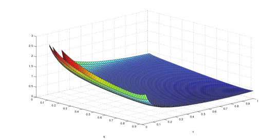
Figure 6: Display of the function $\frac{x^{-0.5}\left(1-q^{3}\frac{x^{3}}{[3]_{q}}\right)_{q^{3}}^{\frac{0.5}{3}-1}}{B_{q,3}(0.5,0.5)[3]_{q}^{\frac{0.5}{3}}}$ for $0\leq q<1$ and $0\leq x\leq 1$.

Our final result provides an explicit formula for the cumulative beta $q$-distribution. If follows as an easy consequence of the definition of the Jackson integral and the definition of $B_{q,k}(t,s)$.

Theorem 9.

The cumulative beta $q$-distribution is given by

$$\frac{1}{B_{q,k}(t,s)[k]_{q}^{\frac{t}{k}}}\int_{0}^{x}s^{t-1}\left(1-q^{k}\frac{s^{k}}{[k]_{q}}\right)_{q^{k}}^{\frac{s}{k}-1}d_{q}x=\frac{(1-q)x^{t}}{B_{q,k}(t,s)[k]_{q}^{\frac{t}{k}}}\sum_{n=0}^{\infty}q^{nt}\left(1-q^{k(n+1)}\frac{x^{k}}{[k]_{q}}\right)_{q^{k}}^{\frac{s}{k}-1}.$$

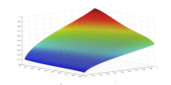
Figure 7: Cumulative distribution of the $q$-density $\frac{x^{-0.5}\left(1-q^{3}\frac{x^{3}}{[3]_{q}}\right)_{q^{3}}^{\frac{0.5}{3}-1}}{B_{q,3}(0.5,0.5)[3]_{q}^{\frac{0.5}{3}}}$ for $0\leq q<1$ and $0\leq x\leq 1$.

ragadiaz@gmail.com
Instituto de Matemáticas y sus Aplicaciones, Universidad Sergio Arboleda, Bogotá, Colombia

camiloortiz@javeriana.edu.co,    epariguan@javeriana.edu.co
Departamento de Matemáticas, Pontificia Universidad Javeriana, Bogotá, Colombia

References

- [1] Andrews G., Askey R., Roy R., Special Functions, Cambridge Univ. Press, Cambridge, 1999.
- [2] Callan D., A Combinatorial Survey of Identities for the Double Factorial, preprint available at http://arxiv.org/abs/0906.1317.
- [3] Cheung P., Kac V., Quantum Calculus, Springer-Verlag, Berlin, 2002.
- [4] De Sole A., Kac V., On integral representations of -gamma and -beta functions, Atti. Accad. Naz. Lincei Cl. Sci. Fis. Mat. Natur. Rend. Lincei 9. Mat. Appl., 2005, 16, 11-29.
- [5] Díaz R., Pariguan E., On hypergeometric functions and Pochhammer -symbol, Divulg. Mat., 2007, 15, 179-192.
- [6] Díaz R., Pariguan E., On the Gaussian -distribution, J. Math. Anal. Appl., 2009, 358, 1-9.
- [7] Diaz R., Pariguan E., Super, Quantum and Non-Commutative Species, Afr. Diaspora J. Math, 2009, 8, 90-130.
- [8] Díaz R., Teruel C., -generalized gamma and beta functions, J. Nonlinear Math. Phys., 2005, 12, 118 - 134.
- [9] George G., Mizan R., Basic Hypergeometric series, Cambridge Univ. Press, Cambridge, 1990.
- [10] Gessel I., Stanley R., Stirling polynomials, J. Combin. Theory Ser. A, 1978, 24, 24-33.
- [11] Kokologiannaki C. G., Properties and Inequalities of Generalized k-Gamma, Beta and Zeta Functions, Int. J. Contemp. Math. Sciences, 2010, 5, 653-660.
- [12] Kuba M., On Path diagrams and Stirling permutations, preprint available at http://arxiv4.library.cornell.edu/abs/0906.1672.
- [13] Mansour M., Determining the Generalized Gamma Function by Functional Equations, Int. J. Contemp. Math. Sciences, 2009, 4, 1037-1042.
- [14] Zeilberger D., Enumerative and Algebraic Combinatorics, In: Gowers T. (Ed.), The Princeton Companion to Mathematics, Princeton Univ. Press, Princeton, 2008.