Optimal waveform estimation for classical and quantum systems via time-symmetric smoothing. II. Applications to atomic magnetometry and Hardy’s paradox

Abstract

The quantum smoothing theory [Tsang, Phys. Rev. Lett. 102, 250403 (2009); Phys. Rev. A, in press (e-print arXiv:0906.4133)] is extended to account for discrete jumps in the classical random process to be estimated, discrete variables in the quantum system, such as spin, angular momentum, and photon number, and Poissonian measurements, such as photon counting. The extended theory is used to model atomic magnetometers and study Hardy’s paradox in phase space. In the phase-space picture of Hardy’s proposed experiment, the negativity of the predictive Wigner distribution is identified as the culprit of the disagreement between classical reasoning and quantum mechanics.

I Introduction

In previous papers tsang_prl ; tsang_pra , I have proposed a quantum smoothing theory, which can be used to optimally estimate classical signals coupled to quantum sensors under continuous measurements, such as gravitational wave detectors and atomic magnetometers. Smoothing can be significantly more accurate than current quantum filtering methods belavkin ; carmichael ; gardiner_zoller ; mabuchi ; berry ; thomsen ; geremia ; stockton ; bouten when the classical signal is a stochastic process and delay is permitted in the estimation. While Refs. tsang_prl ; tsang_pra focus on diffusive classical random processes, quantum systems with continuous degrees of freedom, and Gaussian measurements, the aim of this paper is to extend the theory to account for discrete variables in the systems and the measurements. In particular, I shall consider discrete jumps in the classical random process, discrete variables in the quantum system, such as spin, angular momentum, and photon number, and Poissonian measurements, such as photon counting. Such extensions are especially important for the modeling of atomic magnetometry thomsen ; geremia ; stockton ; budker ; kuzmich ; petersen ; bouten .

In the case of atomic magnetometry, the importance of estimation delay was discovered by Petersen and Mølmer petersen , who found that the estimation of a fluctuating magnetic field modeled as an Ornstein-Uhlenbeck process becomes more accurate when the estimation is delayed and observations at later times are taken into account. I shall generalize their results using the quantum smoothing theory, derive the optimal strategy of delayed estimation for atomic magnetometry, and discuss practical methods of implementing the strategy.

A different kind of estimation problem comes up in Hardy’s paradox hardy , in which one estimates the positions of an electron and a positron in interferometers based on posterior measurement outcomes and obtains paradoxical results. I shall demonstrate that the salient features of the paradox can be reproduced mathematically using the quantum smoothing theory in discrete phase space, which is arguably the most natural way of modeling classical properties of quantum objects. It is shown that the negativity of the predictive Wigner distribution can be regarded as the culprit of the disagreement between classical reasoning and quantum mechanics. This phase-space approach is somewhat different from Aharonov et al.’s weak value approach aav_hardy . Whether the two can be reconciled remains to be seen.

This paper is organized as follows: Section II reviews the classical filtering and smoothing equations when the system process has jumps and the observations have Poissonian statistics, as derived by Snyder snyder ; snyder_book and Pardoux pardoux_poisson . Section III generalizes such equations to the quantum regime for smoothing of classical random processes coupled to quantum systems. Sec. IV converts the quantum equations to equivalent phase-space equations for discrete Wigner distributions. Sec. V studies the application of the theory to atomic magnetometry. Sec. VI studies Hardy’s paradox using quantum smoothing in discrete phase space.

II Classical filtering and smoothing for Poissonian observations

Define $x_{t}$ as the classical system random process, the a priori probability density of which satisfies the differential Chapman-Kolmogorov equation gardiner

$$\frac{\partial P(x,t)}{\partial t} =\mathcal{L}_{C}P(x,t),$$ (1)

$$\mathcal{L}_{C}P(x,t) \equiv-\sum_{\mu}\frac{\partial}{\partial x_{\mu}}\left[A_{\mu}P(x,t)\right]$$

$$\quad+\frac{1}{2}\sum_{\mu,\nu}\frac{\partial^{2}}{\partial x_{\mu}\partial x_{\nu}}\left[B_{\mu\nu}P(x,t)\right]$$

$$\quad+\int dx^{\prime}\big{[}J(x|x^{\prime},t)P(x^{\prime},t)-J(x^{\prime}|x,t)P(x,t)\big{]},$$ (2)

where $J(x|x^{\prime},t)$ is the probability density per unit time that $x_{t}$ will jump from $x^{\prime}$ to $x$. For an obseration process with Poissonian noise, the conditional probability density is

$$P(\delta N_{\mu t}|x_{t}) =\exp\left[-\lambda_{\mu}(x_{t},t)\delta t\right]\frac{[\lambda_{\mu}(x_{t},t)\delta t]^{\delta N_{\mu}}}{\delta N_{\mu}!},$$ (3)

with the continuous-time limit

$$dN_{\mu t}^{2} =dN_{\mu t},$$ (4)

$$P(dN_{\mu t}=0|x_{t}) =1-\lambda_{\mu}(x_{t},t)dt,$$ (5)

$$P(dN_{\mu t}=1|x_{t}) =\lambda_{\mu}(x_{t},t)dt.$$ (6)

Defining the observation record in the time interval $t_{0}\leq t<t$ as

$$dN_{[t_{0},t)} =\left\{dN_{t},t_{0}\leq t<t\right\}$$ (7)

and the filtering probability density as the probability density of $x_{t}$ conditioned upon past observations, given by

$$F(x,t) \equiv P(x_{t}=x|dN_{[t_{0},t)}),$$ (8)

the Itō stochastic differential equation for $F(x,t)$ is called the Snyder equation and given by snyder ; snyder_book

$$dF =dt\mathcal{L}_{C}F+\sum_{\mu}\left(dN_{\mu t}-dt\left\langle\lambda_{\mu}\right\rangle_{F}\right)\left\langle\lambda_{\mu}\right\rangle_{F}^{-1}$$

$$\quad\times\left(\lambda_{\mu}-\left\langle\lambda_{\mu}\right\rangle_{F}\right)F,$$ (9)

$$\left\langle\lambda_{\mu}\right\rangle_{F} \equiv\int dx\lambda_{\mu}(x,t)F(x,t).$$ (10)

A linear equation for an unnormalized $F(x,t)$ was derived by Pardoux and given by pardoux_poisson

$$df =dt\mathcal{L}_{C}f+\sum_{\mu}\left(dN_{\mu t}-dt\right)(\lambda_{\mu}-1)f,$$ (11)

with

$$F(x,t) =\frac{f(x,t)}{\int dxf(x,t)}.$$ (12)

To perform smoothing in the time-symmetric form pardoux_poisson , first solve for an unnormalized retrodictive likelihood function $P(dN_{[t,T)}|x_{t}=x)\propto g(x,t)$ using the adjoint of Eq. (11),

$$-dg =dt\mathcal{L}_{C}^{*}g+\sum_{\mu}\left(dN_{\mu t}-dt\right)(\lambda_{\mu}-1)g,$$ (13)

to be solved backward in time with final condition $g(x,T)\propto 1$. The smoothing probability density at time $\tau$ given the observation record $dN_{[t_{0},T)}$ in the time interval $t_{0}\leq\tau\leq T$ is then

$$P(x_{\tau}=x|dN_{[t_{0},T)}) =\frac{g(x,\tau)f(x,\tau)}{\int dxg(x,\tau)f(x,\tau)}.$$ (14)

III Hybrid classical-quantum filtering and smoothing for Poissonian observations

Using the same approach as Refs. tsang_prl ; tsang_pra , it is not difficult to generalize the above classical equations to the quantum regime for hybrid classical-quantum filtering and smoothing. Define $x_{t}$ as the classical system process that one wishes to estimate, which is coupled to a quantum system under measurements. As before, the quantum backaction from the quantum system to the classical one is assumed to be negligible. Define the hybrid density operator that describes the joint statistics of the classical and quantum systems hybrid as $\hat{\rho}(x,t)$. The a priori evolution of $\hat{\rho}(x_{t},t)$ is governed by

$$\frac{\partial\hat{\rho}(x,t)}{\partial t} =\mathcal{L}\hat{\rho}(x,t),$$ (15)

$$\mathcal{L}\hat{\rho}(x,t) \equiv\mathcal{L}_{0}\hat{\rho}(x,t)+\mathcal{L}_{I}(x)\hat{\rho}(x,t)+\mathcal{L}_{C}\hat{\rho}(x,t),$$ (16)

where $\mathcal{L}_{0}$ is the superoperator that governs the evolution of the quantum system, $\mathcal{L}_{I}$ is the superoperator that describes the coupling of the classical system to the quantum system, via an interaction Hamiltonian for example, and $\mathcal{L}_{\textrm{C}}$ is the Chapman-Kolmogorov operator defined by Eq. (2). The measurement, on the other hand, is described by the quantum Bayes theorem,

$$\hat{\rho}(x_{t}|\delta N_{\mu t}) =\frac{\hat{M}(\delta N_{\mu t}|x_{t})\hat{\rho}(x_{t})\hat{M}^{\dagger}(\delta N_{\mu t}|x_{t})}{\int dx_{t}\operatorname{tr}(\textrm{numerator})},$$ (17)

where the measurement operator with Poissonian statistics is

$$\hat{M}(\delta N_{\mu t}|x_{t}) =\exp\left[-\frac{1}{2}\hat{L}_{\mu}^{\dagger}(x_{t},t)\hat{L}_{\mu}(x_{t},t)\delta t\right]$$

$$\quad\times\frac{[\hat{L}_{\mu}(x_{t},t)\sqrt{\delta t}]^{\delta N_{\mu t}}}{\sqrt{\delta N_{\mu t}!}},$$ (18)

where $\hat{L}_{\mu}(x_{t},t)$ is a hybrid operator, an annihilation operator for example, and can also depend on $x_{t}$. In the continuous-time limit,

$$\hat{M}(dN_{\mu t}=0|x_{t}) =\hat{1}-\frac{1}{2}\hat{L}_{\mu}^{\dagger}(x_{t},t)\hat{L}_{\mu}(x_{t},t)dt,$$ (19)

$$\hat{M}(dN_{\mu t}=1|x_{t}) =\hat{L}_{\mu}(x_{t},t)\sqrt{dt}.$$ (20)

After some algebra, the stochastic differential equation for the filtering hybrid density operator, defined as

$$\hat{F}(x,t) \equiv\hat{\rho}(x_{t}=x|dN_{[t_{0},t)}),$$ (21)

is given by gardiner_zoller ; holevo

$$d\hat{F} =dt\mathcal{L}\hat{F}+dt\sum_{\mu}\left(\hat{L}_{\mu}\hat{F}\hat{L}_{\mu}^{\dagger}-\frac{1}{2}\hat{L}_{\mu}^{\dagger}\hat{L}_{\mu}\hat{F}-\frac{1}{2}\hat{F}\hat{L}_{\mu}^{\dagger}\hat{L}_{\mu}\right)$$

$$\quad+\sum_{\mu}\left(dN_{\mu t}-dt\left\langle\hat{L}_{\mu}^{\dagger}\hat{L}_{\mu}\right\rangle_{\hat{F}}\right)\left\langle\hat{L}_{\mu}^{\dagger}\hat{L}_{\mu}\right\rangle_{\hat{F}}^{-1}$$

$$\quad\times\left(\hat{L}_{\mu}\hat{F}\hat{L}_{\mu}^{\dagger}-\left\langle\hat{L}_{\mu}^{\dagger}\hat{L}_{\mu}\right\rangle_{\hat{F}}\hat{F}\right),$$ (22)

where

$$\left\langle\hat{L}_{\mu}^{\dagger}\hat{L}_{\mu}\right\rangle_{\hat{F}} \equiv\int dx\operatorname{tr}\left[\hat{L}_{\mu}^{\dagger}(x,t)\hat{L}_{\mu}(x,t)\hat{F}(x,t)\right].$$ (23)

Equation (22) is a quantum generalization of the Snyder equation [Eq. (9)]. A linear version of Eq. (22), analogous to Eq. (11), may be written as holevo

$$d\hat{f} =dt\mathcal{L}\hat{f}+dt\sum_{\mu}\left(\hat{L}_{\mu}\hat{f}\hat{L}_{\mu}^{\dagger}-\frac{1}{2}\hat{L}_{\mu}^{\dagger}\hat{L}_{\mu}\hat{f}-\frac{1}{2}\hat{f}\hat{L}_{\mu}^{\dagger}\hat{L}_{\mu}\right)$$

$$\quad+\sum_{\mu}\left(dN_{\mu t}-dt\right)\left(\hat{L}_{\mu}\hat{f}\hat{L}_{\mu}^{\dagger}-\hat{f}\right),$$ (24)

$$\hat{F}(x,t) =\frac{\hat{f}(x,t)}{\int dx\operatorname{tr}[\hat{f}(x,t)]}.$$ (25)

The classical incoherent limit of Eq. (24) is obviously Eq. (11), and Eq. (24) can be verified against Eq. (22) by normalizing the former using Itō rule.

To perform smoothing, one also needs to solve for the unnormalized hybrid effect operator $\hat{E}(dN_{[t,T)}|x_{t}=x)\propto\hat{g}(x,t)$ using the adjoint of Eq. (24) tsang_prl ; tsang_pra ,

$$-d\hat{g} =dt\mathcal{L}^{*}\hat{g}+dt\sum_{\mu}\left(\hat{L}_{\mu}^{\dagger}\hat{g}\hat{L}_{\mu}-\frac{1}{2}\hat{g}\hat{L}_{\mu}^{\dagger}\hat{L}_{\mu}-\frac{1}{2}\hat{L}_{\mu}^{\dagger}\hat{L}_{\mu}\hat{g}\right)$$

$$\quad+\sum_{\mu}\left(dN_{\mu t}-dt\right)\left(\hat{L}_{\mu}^{\dagger}\hat{g}\hat{L}_{\mu}-\hat{g}\right),$$ (26)

where the final condition is $\hat{g}(x,T)\propto\hat{1}$ and the adjoint is defined with respect to the Hilbert-Schmidt inner product

$$\left\langle\hat{g}(x,t),\hat{f}(x,t)\right\rangle \equiv\int dx\operatorname{tr}\left[\hat{g}(x,t)\hat{f}(x,t)\right],$$ (27)

$$\left\langle\hat{g}(x,t),\mathcal{L}\hat{f}(x,t)\right\rangle =\left\langle\mathcal{L}^{*}\hat{g}(x,t),\hat{f}(x,t)\right\rangle.$$ (28)

The smoothing probability density is then

$$h(x,\tau)\equiv P(x_{\tau}=x|dN_{[t_{0},T)}) =\frac{\operatorname{tr}[\hat{g}(x,\tau)\hat{f}(x,\tau)]}{\int dx\operatorname{tr}[\hat{g}(x,\tau)\hat{f}(x,\tau)]}.$$ (29)

Incorporating the Gaussian measurements considered in Refs. tsang_prl ; tsang_pra into the equations above is straightforward. This is useful, for example, when both photon counting and homodyne detection are performed in a quantum optics experiment foster . With Poissonian observations $dN_{t}$ and Gaussian observations $dy_{t}$, the resulting filtering equation for $\hat{F}(x,t)$ is

$$d\hat{F} =dt\mathcal{L}\hat{F}+dt\sum_{\mu}\left(\hat{L}_{\mu}\hat{F}\hat{L}_{\mu}^{\dagger}-\frac{1}{2}\hat{L}_{\mu}^{\dagger}\hat{L}_{\mu}\hat{F}-\frac{1}{2}\hat{F}\hat{L}_{\mu}^{\dagger}\hat{L}_{\mu}\right)$$

$$\quad+\frac{dt}{8}\left(2\hat{C}^{T}R^{-1}\hat{F}\hat{C}^{\dagger}-\hat{C}^{\dagger T}R^{-1}\hat{C}\hat{F}-\hat{F}\hat{C}^{\dagger T}R^{-1}\hat{C}\right)$$

$$\quad+\sum_{\mu}\left(dN_{\mu t}-dt\left\langle\hat{L}_{\mu}^{\dagger}\hat{L}_{\mu}\right\rangle_{\hat{F}}\right)\left\langle\hat{L}_{\mu}^{\dagger}\hat{L}_{\mu}\right\rangle_{\hat{F}}^{-1}$$

$$\quad\times\left(\hat{L}_{\mu}\hat{F}\hat{L}_{\mu}^{\dagger}-\left\langle\hat{L}_{\mu}^{\dagger}\hat{L}_{\mu}\right\rangle_{\hat{F}}\hat{F}\right)$$

$$\quad+\frac{1}{2}\left[\left(\hat{C}-\langle\hat{C}\rangle_{\hat{F}}\right)^{T}R^{-1}d\eta_{t}\hat{F}+\textrm{H.c.}\right],$$ (30)

$$d\eta_{t} \equiv dy_{t}-\frac{dt}{2}\left\langle\hat{C}+\hat{C}^{\dagger}\right\rangle_{\hat{F}},$$ (31)

where $\hat{C}=\hat{C}(x,t)$ is a vector of hybrid operators, $R=R(t)$ is a positive-definite matrix, $d\eta_{t}$ is a vectoral Wiener increment with covariance matrix $R(t)dt$, and H. c. denotes Hermitian conjugate.

The equation for $\hat{f}(x,t)$ is

$$d\hat{f} =dt\mathcal{L}\hat{f}+dt\sum_{\mu}\left(\hat{L}_{\mu}\hat{f}\hat{L}_{\mu}^{\dagger}-\frac{1}{2}\hat{L}_{\mu}^{\dagger}\hat{L}_{\mu}\hat{f}-\frac{1}{2}\hat{f}\hat{L}_{\mu}^{\dagger}\hat{L}_{\mu}\right)$$

$$\quad+\frac{dt}{8}\left(2\hat{C}^{T}R^{-1}\hat{f}\hat{C}^{\dagger}-\hat{C}^{\dagger T}R^{-1}\hat{C}\hat{f}-\hat{f}\hat{C}^{\dagger T}R^{-1}\hat{C}\right)$$

$$\quad+\sum_{\mu}\left(dN_{\mu t}-dt\right)\left(\hat{L}_{\mu}\hat{f}\hat{L}_{\mu}^{\dagger}-\hat{f}\right)$$

$$\quad+\frac{1}{2}\left(\hat{C}^{T}R^{-1}dy_{t}\hat{f}+\textrm{H.c.}\right),$$ (32)

and for $\hat{g}(x,t)$,

$$-d\hat{g} =dt\mathcal{L}^{*}\hat{g}+dt\sum_{\mu}\left(\hat{L}_{\mu}^{\dagger}\hat{g}\hat{L}_{\mu}-\frac{1}{2}\hat{g}\hat{L}_{\mu}^{\dagger}\hat{L}_{\mu}-\frac{1}{2}\hat{L}_{\mu}^{\dagger}\hat{L}_{\mu}\hat{g}\right)$$

$$\quad+\frac{dt}{8}\left(2\hat{C}^{\dagger T}R^{-1}\hat{g}\hat{C}-\hat{g}\hat{C}^{\dagger T}R^{-1}\hat{C}-\hat{C}^{\dagger T}R^{-1}\hat{C}\hat{g}\right)$$

$$\quad+\sum_{\mu}\left(dN_{\mu t}-dt\right)\left(\hat{L}_{\mu}^{\dagger}\hat{g}\hat{L}_{\mu}-\hat{g}\right)$$

$$\quad+\frac{1}{2}\left(\hat{g}\hat{C}^{T}R^{-1}dy_{t}+\textrm{H.c.}\right).$$ (33)

IV Quantum smoothing in phase space

One method of solving Eqs. (29), (32), and (33) for hybrid smoothing is to use Wigner distributions tsang_prl ; tsang_pra . For a quantum system with a discrete degree of freedom, such as spin, angular momentum, or an $N$-level system, one may define the discrete Wigner distribution, according to Feynman feynman and Wootters wootters , as

$$f(q,p,x,t) \equiv\frac{1}{N}\operatorname{tr}\left[\hat{f}(x,t)\hat{W}(q,p)\right],$$ (34)

$$q \in\left\{0,1,\dots,N-1\right\},$$ (35)

$$p \in\left\{0,1,\dots,N-1\right\}.$$ (36)

The operator $\hat{W}(q,p)$ for prime $N$ is

$$\quad\hat{W}(q,p)$$

$$\equiv\bigg{\{}\begin{array}[]{cc}\frac{1}{2}\left[(-1)^{q}\hat{\sigma}_{z}+(-1)^{p}\hat{\sigma}_{x}+(-1)^{q+p}\hat{\sigma}_{y}+\hat{1}\right],&N=2;\\ \sum_{q_{1},q2}\delta_{2q,q_{1}+q_{2}}\exp\left[\frac{2\pi i}{N}p(q_{1}-q_{2})\right]|q_{1}\rangle\langle q_{2}|,&N>2.\end{array}$$ (39)

$\hat{\sigma}_{x}$, $\hat{\sigma}_{y}$, and $\hat{\sigma}_{z}$ are Pauli matrices, $|q_{1}\rangle$ and $|q_{2}\rangle$ are eigenstates of $\hat{q}$, and modular arithmetic with modulus $N$ is implicitly assumed. For a nonprime $N$, the system can be decomposed into subsystems with prime $N$’s and the Wigner distribution can be defined using $\hat{W}(q,p)$ for each subsystem wootters .

An alternative definition in a $2N\times 2N$ phase space, first suggested by Hannay and Berry hannay , is

$$\tilde{f}(q,p,x,t) \equiv\frac{1}{2N}\operatorname{tr}\left[\hat{f}(x,t)\hat{w}(q,p)\right],$$

$$q \in\left\{0,\frac{1}{2},\dots,N-\frac{1}{2}\right\},$$

$$p \in\left\{0,\frac{1}{2},\dots,N-\frac{1}{2}\right\},$$

$$\hat{w}(q,p) \equiv\sum_{u}\exp\left(\frac{4\pi ipu}{N}\right)|q+u\rangle\langle q-u|,$$

$$u \in\left\{-\frac{N}{2}+\frac{1}{2},-\frac{N}{2}+1,\dots,\frac{N}{2}\right\},$$ (40)

where the matrix elements with noninteger indices are assumed to be zero. One may also use either Wigner function to describe the energy level $n$ and phase $\phi$ of a harmonic oscillator by letting $n=q$, $\phi=2\pi p/N$, and taking the $N\to\infty$ limit at the end of a calculation vaccaro ; luks .

Both definitions have a particularly desirable property for the purpose of smoothing, namely,

$$\operatorname{tr}\left[\hat{g}(x,t)\hat{f}(x,t)\right] =N\sum_{q,p}g(q,p,x,t)f(q,p,x,t),$$ (41)

$$=2N\sum_{q,p}\tilde{g}(q,p,x,t)\tilde{f}(q,p,x,t),$$ (42)

so the smoothing probability density can be written in terms of the Wigner distributions as

$$h(x,\tau) =\frac{\sum_{q,p}g(q,p,x,\tau)f(q,p,x,\tau)}{\int dx\sum_{q,p}g(q,p,x,\tau)f(q,p,x,\tau)}$$ (43)

or

$$h(x,\tau) =\frac{\sum_{q,p}\tilde{g}(q,p,x,\tau)\tilde{f}(q,p,x,\tau)}{\int dx\sum_{q,p}\tilde{g}(q,p,x,\tau)\tilde{f}(q,p,x,\tau)}.$$ (44)

Equations (43) and (44) become equivalent to the classical smoothing density given by Eq. (14), with the quantum degrees of freedom marginalized, if $f$ and $g$ or $\tilde{f}$ and $\tilde{g}$ are nonnegative and can be regarded as classical probability densities. The hybrid smoothing problem can then be solved using classical filtering and smoothing techniques.

If one desires to obtain smoothing estimates of the quantum degrees of freedom, a quantum smoothing quasiprobability distribution may be defined as

$$h(q,p,x,\tau) =\frac{g(q,p,x,\tau)f(q,p,x,\tau)}{\int dx\sum_{q,p}g(q,p,x,\tau)f(q,p,x,\tau)}$$ (45)

or

$$\tilde{h}(q,p,x,\tau) =\frac{\tilde{g}(q,p,x,\tau)\tilde{f}(q,p,x,\tau)}{\int dx\sum_{q,p}\tilde{g}(q,p,x,\tau)\tilde{f}(q,p,x,\tau)}.$$ (46)

From the perspective of estimation theory, these definitions of quantum smoothing distributions are arguably the most natural, for they both give the correct classical smoothing distribution when the quantum degrees of freedom are marginalized, are equivalent to the smoothing distributions in classical smoothing theory when $f$ and $g$ or $\tilde{f}$ and $\tilde{g}$ are nonnegative, and are explicitly normalized.

There are many other equally qualified definitions of the Wigner distribution in discrete or periodic phase space gibbons ; agarwal . Choosing which definition to use depends on the application. The Feynman-Wootters distribution is defined only on the eigenvalues of $\hat{q}$ and $\hat{p}$, so it appears more physical, but the Hannay-Berry definition is easier to calculate analytically for arbitrary $N$ and, as shown in Appendix A, naturally arises from the statistics of weak measurements.

V Atomic Magnetometry

V.1 Optimal smoothing

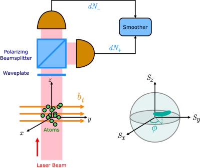
Figure 1: (color online). Left: basic setup of atomic magnetometer as considered in Refs. kuzmich ; geremia ; stockton ; bouten . Right: the spherical phase space for spin.

An important application of quantum estimation theory is atomic magnetometry budker ; kuzmich ; thomsen ; geremia ; stockton ; bouten ; petersen . Consider the setup described in Refs. geremia ; stockton ; bouten ; kuzmich and depicted in Fig. 1. An atomic spin ensemble is initially prepared in a coherent state with the mean collective spin vector along the $x$ axis. Let the magnetic field be polarized along $y$ axis and given by

$$b_{t}\equiv x_{1t},$$ (47)

a component of the classical system process to be estimated. The magnetic field introduces Larmor precession to the spin via the interaction Hamiltonian

$$\hat{H}_{I}(x) =-\gamma b\hat{S}_{y},$$ (48)

$$\mathcal{L}_{I}(x)\hat{F}(x,t) =-\frac{i}{\hbar}\left[\hat{H}_{I}(x),\hat{F}(x,t)\right]=\frac{i\gamma}{\hbar}b\left[\hat{S}_{y},\hat{F}\right],$$ (49)

where $\hat{S}_{y}$ is the $y$ component of the spin vector operator and $\gamma$ is the gyromagnetic ratio. Under continuous optical polarimetry measurements, the stochastic equation for the filtering density operator $\hat{F}(x,t)$ has been derived by Bouten et al. bouten and is given by

$$d\hat{F} =dt\Big{\{}\mathcal{L}_{C}\hat{F}+\frac{i\gamma}{\hbar}b\left[\hat{S}_{y},\hat{F}\right]+|a|^{2}$$

$$\quad\times\left[\cos(\kappa\hat{m})\hat{F}\cos(\kappa\hat{m})+\sin(\kappa\hat{m})\hat{F}\sin(\kappa\hat{m})-\hat{F}\right]\Big{\}}$$

$$\quad+\sum_{\mu=+,-}\left(dN_{\mu t}-dt\left\langle\hat{L}_{\mu}^{\dagger}\hat{L}_{\mu}\right\rangle_{\hat{F}}\right)$$

$$\quad\times\left\langle\hat{L}_{\mu}^{\dagger}\hat{L}_{\mu}\right\rangle_{\hat{F}}^{-1}\left(\hat{L}_{\mu}\hat{F}\hat{L}_{\mu}^{\dagger}-\left\langle\hat{L}_{\mu}^{\dagger}\hat{L}_{\mu}\right\rangle_{\hat{F}}\hat{F}\right),$$ (50)

which is in the form of Eq. (22), with

$$\hat{m} \equiv\frac{\hat{S}_{z}}{\hbar}, \hat{L}_{\pm} =\frac{a}{\sqrt{2}}\left[\cos(\kappa\hat{m})\pm\sin(\kappa\hat{m})\right],$$ (51)

$\kappa$ is the light-spin coupling parameter and $a$ is the normalized optical envelope. The linear predictive and retrodictive equations for $\hat{f}(x,t)$ and $\hat{g}(x,t)$ become

$$d\hat{f} =dt\Big{\{}\mathcal{L}_{C}\hat{f}+\frac{i\gamma}{\hbar}b\left[\hat{S}_{y},\hat{f}\right]+|a|^{2}$$

$$\quad\times\left[\cos(\kappa\hat{m})\hat{f}\cos(\kappa\hat{m})+\sin(\kappa\hat{m})\hat{f}\sin(\kappa\hat{m})-\hat{f}\right]\Big{\}}$$

$$\quad+\sum_{\mu=+,-}\left(dN_{\mu t}-dt\right)\left(\hat{L}_{\mu}\hat{f}\hat{L}_{\mu}^{\dagger}-\hat{f}\right),$$ (52)

$$-d\hat{g} =dt\Big{\{}\mathcal{L}_{C}^{*}\hat{g}-\frac{i\gamma}{\hbar}b\left[\hat{S}_{y},\hat{g}\right]+dt|a|^{2}$$

$$\quad\times\left[\cos(\kappa\hat{m})\hat{g}\cos(\kappa\hat{m})+\sin(\kappa\hat{m})\hat{g}\sin(\kappa\hat{m})-\hat{g}\right]\Big{\}}$$

$$\quad+\sum_{\mu=+,-}\left(dN_{\mu t}-dt\right)\left(\hat{L}_{\mu}^{\dagger}\hat{g}\hat{L}_{\mu}-\hat{g}\right).$$ (53)

After solving Eq. (52) forward in time for $\hat{f}(x,\tau)$ and Eq. (53) backward in time for $\hat{g}(x,\tau)$, the smoothing probability distribution is given by

$$h(x,\tau) =\frac{\operatorname{tr}[\hat{g}(x,\tau)\hat{f}(x,\tau)]}{\int dx\operatorname{tr}[\hat{g}(x,\tau)\hat{f}(x,\tau)]},$$ (54)

which can be used to produce the optimal estimate and the associated error of the system process $x_{\tau}$, including the magnetic field $b_{\tau}\equiv x_{1\tau}$.

V.2 Smoothing in phase space

The usual strategy of solving the quantum estimation problem is to take the $S_{x}\gg S_{y}$, $S_{x}\gg S_{z}$ limit, assume $\hat{S}_{y}$ and $\hat{S}_{z}$ are continuous, and approximate the conditional quantum state as a Gaussian state thomsen ; geremia ; stockton ; kuzmich ; petersen . This is akin to approximating the spherical phase space with a flat one near $\mathbf{S}=(S_{x},0,0)$. While the Gaussian approximation is probably the most practical, in order to illustrate the discrete phase-space formalism proposed in Sec. IV, I shall first attempt to convert Eqs. (52) and (53) to stochastic equations for discrete Wigner distributions in the $2N\times 2N$ phase space before making further approximations.

Let

$$\hat{m} =\hat{q}-s, N =2s+1,$$ (55)

where $s$ is the total spin number. Then

$$\hat{\phi} \equiv\frac{2\pi\hat{p}}{N}$$ (56)

is the operator for the azimuthal angle of the spin vector. I shall use $m$ and $\phi$ as the phase-space variables instead of $q$ and $p$, and let

$$f(m,\phi) =\tilde{f}\left(q=m+s,p=\frac{N\phi}{2\pi}\right).$$ (57)

First consider the measurement-induced decoherence term on the second line of Eq. (52). It can be rewritten as

$$\mathcal{L}_{\textrm{M}}\hat{f} \equiv\frac{1}{2}\left(e^{i\kappa\hat{q}}\hat{f}e^{-i\kappa\hat{q}}+e^{-i\kappa\hat{q}}\hat{f}e^{i\kappa\hat{q}}\right)-\hat{f}.$$ (58)

Using the definition of the discrete Wigner function given by Eqs. (40) and $\stackrel{{\scriptstyle\hat{w}}}{{\to}}$ to denote the transform to the $2N\times 2N$ phase space, it can be shown that

$$\mathcal{L}_{\textrm{M}}\hat{f}\stackrel{{\scriptstyle\hat{w}}}{{\to}} \sum_{\phi^{\prime}}J(\phi-\phi^{\prime})f(m,\phi^{\prime},x,t)-f(m,\phi,x,t),$$ (59)

where

$$J(\phi-\phi^{\prime}) \equiv\frac{1}{4N}\bigg{\{}\frac{\sin[N(\phi-\phi^{\prime}-\kappa)]}{\tan[(\phi-\phi^{\prime}-\kappa)/2]}$$

$$\quad\frac{\sin[N(\phi-\phi^{\prime}+\kappa)]}{\tan[(\phi-\phi^{\prime}+\kappa)/2]}\bigg{\}}.$$ (60)

While Eq. (59) has the appearance of the jump term in the Chapman-Kolmogorov equation [Eq. (2)], $J(\phi-\phi^{\prime})$, which plays the role of a jump probability density, can become negative. In the special case of $\kappa=\pi\mu/N$, where $\mu$ is an integer, however, $J(\phi-\phi^{\prime})$ is simplified to

$$J(\phi-\phi^{\prime}) =\frac{1}{2}\left(\delta_{\phi-\phi^{\prime},\kappa}+\delta_{\phi-\phi^{\prime},-\kappa}\right),$$ (61)

and the measurement-induced decoherence introduces random azimuthal jumps in steps of $\kappa$ to the spin vector around the $z$ axis. In the limit of $N\to\infty$, $\phi$ becomes approximately continuous, $\kappa\approx\pi\mu/N$, and Eq. (59) can be rewritten as

$$\mathcal{L}_{\textrm{M}}\hat{f} \stackrel{{\scriptstyle\hat{w}}}{{\to}}\frac{1}{2}\Big{[}f(m,\phi+\kappa,x,t)+f(m,\phi-\kappa,x,t)\Big{]}$$

$$\quad-f(m,\phi,x,t).$$ (62)

The $N\to\infty$ limit is akin to approximating the spin system as a harmonic oscillator vaccaro and the spherical phase space as a cylindrical one. If $\kappa\ll\langle\Delta\hat{\phi}^{2}\rangle^{1/2}$, we can further make the diffusive approximation:

$$\mathcal{L}_{\textrm{M}}\hat{f} \stackrel{{\scriptstyle\hat{w}}}{{\to}}\frac{\kappa^{2}}{2}\frac{\partial^{2}}{\partial\phi^{2}}f(m,\phi,x,t).$$ (63)

Next, consider the Larmor precession term $(i\gamma/\hbar)b[\hat{S}_{y},\hat{f}]$. In terms of $\hat{m}$ and $\hat{\phi}$,

$$\hat{S}_{y} =\frac{\hbar}{2i}\Big{[}\exp(-i\hat{\phi})\sqrt{s(s+1)-\hat{m}(\hat{m}+1)}$$

$$\quad-\exp(i\phi)\sqrt{s(s+1)-\hat{m}(\hat{m}-1)}\Big{]}.$$ (64)

With this form, it is difficult to convert the Larmor precession term to the phase-space picture analytically, so we again make the cylindrical phase-space approximation with $s\gg\langle\hat{m}\rangle,\langle\Delta\hat{m}^{2}\rangle^{1/2}$, so that the spin vector distribution is concentrated near the equator. This approximation is valid when the magnetic field is small and fluctuating around zero, or a control, such as an applied magnetic field thomsen ; geremia ; stockton or an adjustable direction of the optical beam, is present to realign the spin vector with respect to the optical beam propagation direction. Then

$$\hat{S}_{y} \approx-\hbar s\sin\hat{\phi},$$ (65)

$$\mathcal{L}_{I}\hat{f} \stackrel{{\scriptstyle\hat{w}}}{{\to}}-\gamma bs\cos\phi\left[f(m+\frac{1}{2},\phi,x,t)-f(m-\frac{1}{2},\phi,x,t)\right].$$ (66)

Although this looks like the jump term in Eq. (2), the apparent jump probability density is again negative. To make the classical connection, assume that $m$ is continuous and approximate the difference as a derivative:

$$\mathcal{L}_{I}\hat{f} \stackrel{{\scriptstyle\hat{w}}}{{\to}}-\gamma bs\cos\phi\frac{\partial}{\partial m}f(m,\phi,x,t),$$ (67)

which becomes equivalent to the drift term in Eq. (2) with $A_{m}=\gamma bs\cos\phi$.

Finally, let us consider the terms $\hat{L}_{\pm}\hat{f}\hat{L}_{\pm}^{\dagger}$ in Eq. (52). It is not difficult to show that, in the continuous $\phi$ limit,

$$\hat{L}_{\pm}\hat{f}\hat{L}_{\pm}^{\dagger} \stackrel{{\scriptstyle\hat{w}}}{{\to}}|a|^{2}\bigg{\{}\frac{1}{2}\left[f(m,\phi+\kappa,x,t)+f(m,\phi-\kappa,x,t)\right]$$

$$\quad\pm\sin(2\kappa m)f(m,\phi,x,t)\bigg{\}}.$$ (68)

These terms do not have exact analogs in the corresponding classical equation [Eq. (11)], unless we make the $\kappa\ll\langle\Delta\hat{\phi}^{2}\rangle^{1/2}$ approximation,

$$\hat{L}_{\pm}\hat{f}\hat{L}_{\pm}^{\dagger} \stackrel{{\scriptstyle\hat{w}}}{{\to}}|a|^{2}\bigg{\{}f(m,\phi,x,t)+\frac{\kappa^{2}}{2}\frac{\partial^{2}}{\partial\phi^{2}}f(m,\phi,x,t)$$

$$\quad\pm\sin(2\kappa m)f(m,\phi,x,t)\bigg{\}}$$ (69)

$$\approx|a|^{2}\left[1\pm\sin(2\kappa m)\right]f(m,\phi,x,t).$$ (70)

Summarizing, a classical model of atomic magnetometry can be obtained if we approximate the spherical phase space as a cylindrical one near the equator, assume $m$ is continuous, and let $\kappa\ll\langle\Delta\hat{\phi}^{2}\rangle^{1/2}$. The resulting equations for $f(m,\phi,x,t)$ and $g(m,\phi,x,t)$ are

$$df =dt\left(\mathcal{L}_{C}f-\gamma bs\cos\phi\frac{\partial f}{\partial m}+\frac{|a|^{2}\kappa^{2}}{2}\frac{\partial^{2}f}{\partial\phi^{2}}\right)$$

$$\quad+\sum_{\mu=+,-}(dN_{\mu}-dt)(\lambda_{\mu}-1)f,$$ (71)

$$-dg =dt\left(\mathcal{L}_{C}^{*}g+\gamma bs\cos\phi\frac{\partial g}{\partial m}+\frac{|a|^{2}\kappa^{2}}{2}\frac{\partial^{2}g}{\partial\phi^{2}}\right)$$

$$\quad+\sum_{\mu=+,-}(dN_{\mu}-dt)(\lambda_{\mu}-1)g,$$ (72)

$$\lambda_{\pm} =|a|^{2}\left[1\pm\sin(2\kappa m)\right].$$ (73)

The equivalent system equations are then

$$dx_{t} =A(x_{t},t)dt+B(x_{t},t)dW_{t},$$ (74)

$$dm_{t} =dt\gamma b_{t}s\cos\phi_{t},$$ (75)

where $dW_{t}$ and $d\phi_{t}$ are independent Wiener increments with $dW_{t}dW_{t}^{T}=Q(t)dt$ and $d\phi_{t}^{2}=|a|^{2}\kappa dt$. Unlike the Gaussian model geremia ; stockton ; petersen , this slightly more general model shows that the $z$ component of the spin is coupled to $\phi_{t}$ via Larmor precession, as one would expect from classical dynamics, since $S_{x}\approx\hbar s\cos\phi$ when $s\gg m$. The diffusion of $\phi$ would therefore reduce the estimation accuracy in the long run.

To make the Gaussian approximation, let $\langle\hat{\phi}_{t}\rangle,\langle\Delta\hat{\phi}_{t}^{2}\rangle^{1/2}\ll 1$, so that $\cos\phi_{t}\approx 1$, and let $x_{t}$ be a Gaussian random process, such as the Ornstein-Uhlenbeck process stockton ; petersen . If $\kappa\langle\hat{m}\rangle,\kappa\langle\Delta\hat{m}^{2}\rangle^{1/2}\ll 1$, and the effective noise covariances are $\langle\lambda_{\pm}\rangle\approx|a|^{2}$, one can use the linear Mayne-Fraser-Potter smoother tsang_pra ; mayne ; tsang_pra2 , which combines the estimates and covariances from a predictive Kalman filter and a retrodictive Kalman filter, to produce the optimal estimate of $x_{t}$. Other equivalent linear smoothers may also be used tsang_pra2 .

VI Hardy’s paradox in phase space

In this section, I shall study Hardy’s paradox hardy in phase space using the quantum smoothing quasiprobability distribution defined by Eq. (45), which allows one to estimate quantum degrees of freedom given past and future observations in a way closely resembling classical estimation theory. The more physical and intuitive Feynman-Wootters distribution is used, since its elements all correspond to actual paths in the setup. I shall show that the paradox arises because the predictive Wigner distribution becomes negative, and quantum mechanics becomes incompatible with classical estimation as a result. This approach is somewhat different from Aharonov et al.’s attempt to explain Hardy’s paradox using weak values aav_hardy .

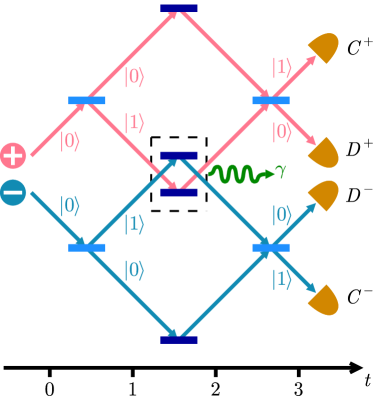
Figure 2: (Color online). Setup of Hardy’s paradox.

As a brief review of the paradox, consider two Mach-Zehnder interferometers, one for a positron and one for an electron, depicted in Fig. 2. If the interferometers are physically separate, then the setup can be configured so that the particles always arrive at the $C^{+}$ and $C^{-}$ detectors, respectively. Now let’s make one arm of an interferometer to overlap with an arm of the other. After the first pair of beamsplitters, the two particles may meet in the overlapping arms, in which case they annihilate each other with probability $1$. With this overlapping setup, there is a $1/16$ probability that the particles will arrive at $D^{+}$ and $D^{-}$, respectively, according to quantum theory.

The paradox arises when one tries to use classical reasoning to estimate which arms the particles went through. If $D^{+}$ detects a positron, then the electron must have been in the overlapping arm to somehow influence the positron to go to $D^{+}$ instead of $C^{+}$. The same reasoning can be applied when $D^{-}$ detects an electron, which should mean that the positron was in the overlapping arm. But if both particles went through the overlapping arms, they should have annihilated each other and would not have been detected.

Denote the position of a particle in one arm as $0$ and that in the other arm as $1$, as shown in Fig. 2. At the time instant labeled $0$,

$$|\Psi\rangle_{0} =|0,0\rangle,$$ (76)

where the first number in the ket denotes the position of the positron, the second number denotes that of the electron, and the subscript is the time label. The corresponding two-particle Wigner distribution using Eqs. (34) and (39) is

$$\quad f_{0}(q^{+},q^{-},p^{+},p^{-})$$

$$=\left(\begin{array}[]{cccc}f_{0}(0,0,0,0)&f_{0}(0,0,0,1)&f_{0}(0,0,1,0)&f_{0}(0,0,1,1)\\ f_{0}(0,1,0,0)&f_{0}(0,1,0,1)&f_{0}(0,1,1,0)&f_{0}(0,1,1,1)\\ f_{0}(1,0,0,0)&f_{0}(1,0,0,1)&f_{0}(1,0,1,0)&f_{0}(1,0,1,1)\\ f_{0}(1,1,0,0)&f_{0}(1,1,0,1)&f_{0}(1,1,1,0)&f_{0}(1,1,1,1)\end{array}\right)$$ (81)

$$=\frac{1}{4}\left(\begin{array}[]{cccc}1&1&1&1\\ 0&0&0&0\\ 0&0&0&0\\ 0&0&0&0\end{array}\right).$$ (86)

After the first pair of beamsplitters,

$$|\Psi\rangle_{1} =\frac{1}{2}\left(|0,0\rangle+|0,1\rangle+|1,0\rangle+|1,1\rangle\right),$$ (87)

$$f_{1}(q^{+},q^{-},p^{+},p^{-}) =\frac{1}{4}\left(\begin{array}[]{cccc}1&0&0&0\\ 1&0&0&0\\ 1&0&0&0\\ 1&0&0&0\end{array}\right).$$ (92)

If the annihilation did not occur, the a posteriori quantum state is

$$|\Psi\rangle_{2} =\frac{1}{\sqrt{3}}\left(|0,0\rangle+|0,1\rangle+|1,0\rangle\right),$$ (93)

$$f_{2}(q^{+},q^{-},p^{+},p^{-}) =\frac{1}{12}\left(\begin{array}[]{cccc}4&0&0&0\\ 2&0&2&0\\ 2&2&0&0\\ 1&-1&-1&1\end{array}\right).$$ (98)

The Wigner distribution has negative elements and can no longer be regarded as a classical phase-space probability distribution. The negative elements, as one shall see later, can be regarded as the culprits that cause the paradox. The predictive marginal distributions are still nonnegative, however. In particular,

$$f_{2}(q^{+},q^{-}) \equiv\sum_{p^{+},p^{-}}f_{2}(q^{+},q^{-},p^{+},p^{-})$$ (99)

$$=\left(\begin{array}[]{c}f_{2}(0,0)\\ f_{2}(0,1)\\ f_{2}(1,0)\\ f_{2}(1,1)\end{array}\right)=\frac{1}{3}\left(\begin{array}[]{c}1\\ 1\\ 1\\ 0\end{array}\right),$$ (108)

which correctly predicts the a posteriori position probability distribution if one measures the positions of the particles at that instant using strong measurements. Most importantly, $f_{2}(1,1)=0$, and the probability that one measures both particles in the overlapping arms with strong measurements is zero.

Now perform retrodiction. Given that $D^{+}$ and $D^{-}$ click, it can be shown that

$$g_{2}(q^{+},q^{-},p^{+},p^{-}) =\frac{1}{4}\left(\begin{array}[]{cccc}0&0&0&1\\ 0&0&0&1\\ 0&0&0&1\\ 0&0&0&1\end{array}\right).$$ (113)

The smoothing quasiprobability distribution at time instant $2$ becomes

$$h_{2}(q^{+},q^{-},p^{+},p^{-}) \propto f_{2}(q^{+},q^{-},p^{+},p^{-})g_{2}(q^{+},q^{-},p^{+},p^{-})$$ (114)

$$=\left(\begin{array}[]{cccc}0&0&0&0\\ 0&0&0&0\\ 0&0&0&0\\ 0&0&0&1\end{array}\right),$$ (119)

$$h_{2}(q^{+},q^{-}) =\left(\begin{array}[]{c}0\\ 0\\ 0\\ 1\end{array}\right).$$ (124)

Hence, given that the annihilation did not occur and $D^{+}$ and $D^{-}$ click, both particles “reappear” in the overlapping arms according to quantum smoothing. This result is consistent with the classical logic that leads one to the same paradoxical conclusion. Mathematically, the paradox arises because the filtering estimation according to $f_{2}(q^{+},q^{-})$ contradicts the smoothing estimation according to $h_{2}(q^{+},q^{-})$, with the former ascertaining that the particles cannot both be in the overlapping arms, while the latter insisting the opposite.

To see why this cannot happen in classical estimation theory, assume for the time being that $f_{2}(q^{+},q^{-},p^{+},p^{-})$ is nonnegative. Then $f_{2}(1,1)$ is zero if and only if $f_{2}(1,1,p^{+},p^{-})$ is zero for all $p^{+}$ and $p^{-}$. If $f_{2}(1,1,p^{+},p^{-})$ is zero, so are $h_{2}(1,1,p^{+},p^{-})$ and $h_{2}(1,1)$ according to Eq. (114). In other words, in classical estimation, if filtering estimates that the two particles cannot both be in the overlapping arms, then no amount of smoothing afterwards can alter the certainty of this fact.

Quantum smoothing, on the other hand, is able to overrule quantum filtering because some elements of $f_{2}(1,1,p^{+},p^{-})$ are negative. This way $f_{2}(1,1)$ can still be zero with nonzero $f_{2}(1,1,p^{+},p^{-})$ elements, and $h_{2}(1,1,p^{-},p^{+})$ and $h_{2}(1,1)$, conditioned upon the detection outcomes, can become nonzero. The negative elements of $f_{2}(q^{+},q^{-},p^{+},p^{-})$ thus cause filtering and smoothing to produce contradictory trajectories.

If the detection outcomes are different, say, $C^{+}$ and $D^{-}$ click, then

$$g_{2}(q^{+},q^{-},p^{+},p^{-}) =\frac{1}{4}\left(\begin{array}[]{cccc}0&1&0&0\\ 0&1&0&0\\ 0&1&0&0\\ 0&1&0&0\end{array}\right),$$ (129)

$$h_{2}(q^{+},q^{-},p^{+},p^{-}) =\left(\begin{array}[]{cccc}0&0&0&0\\ 0&0&0&0\\ 0&2&0&0\\ 0&-1&0&0\end{array}\right),$$ (134)

$$h_{2}(q^{+},q^{-}) =\left(\begin{array}[]{c}0\\ 0\\ 2\\ -1\end{array}\right),$$ (139)

and we have a negative “probability.” Leaving aside the question of interpreting a negative probability feynman , $h_{2}(q^{+},q^{-})$ still suggests that the most likely positions are $(q^{+},q^{-})=(1,0)$, which are consistent with classical reasoning and do not contradict the filtering results indicated by $f_{2}(q^{+},q^{-})$. Similarly, when $C^{+}$ and $C^{-}$ click, the most likely $(q^{+},q^{-})$ according to $h_{2}(q^{-},q^{+})$ is $(0,0)$, which is again what one would expect from a classical argument. In this example at least, the most likely positions suggested by quantum smoothing coincide with the ones obtained by qualitative classical reasoning, as depicted in Fig. 3.

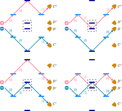
Figure 3: (color online). The most likely paths undertaken by the particles indicated by quantum smoothing given the detection outcomes, provided that annihilation did not occur. These paths coincide with those suggested by qualitative classical reasoning. When $D^{+}$ and $D^{-}$ click, the estimated paths, as shown in the bottom-right figure, contradict with the fact that annihilation did not occur and the two particles could not have both been in the overlapping arms.

To summarize, quantum phase-space filtering and smoothing are able to reproduce mathematically the salient features of Hardy’s paradox and identify the negativity of $f_{2}(q^{+},q^{-},p^{+},p^{-})$ as the culprit that makes the classical phase-space picture and quantum theory incompatible.

VII Conclusion

In conclusion, the time-symmetric smoothing theory is extended to account for discrete variables in classical systems, quantum systems, and observations. To illustrate the extended theory, atomic magnetometry and Hardy’s paradox are studied using quantum phase-space smoothing. The generalized smoothing theory outlined in this paper is expected to be useful in future quantum sensing and information processing applications.

Appendix A Obtaining the quantum smoothing distribution by weak measurements

In the case of continuous variables, the quantum smoothing distribution can be obtained from the statistics of weak position and momentum measurements, conditioned upon past and future observations tsang_pra . One may also apply a similar method to the discrete-variable case. Interestingly, the statistics of weak measurements naturally lead to a $2N\times 2N$ phase space.

Consider consecutive $q$ and $p$ measurements of a quantum system. Let the measurement operators be

$$\hat{M}(y_{q}) =\sqrt{\mathcal{C}}\sum_{q=0}^{N-1}\exp\left[\frac{\epsilon}{2}\cos\frac{2\pi}{N}(y_{q}-q)\right]|q\rangle\langle q|,$$ (140)

$$\hat{M}(y_{p}) =\sqrt{\mathcal{C}}\sum_{p=0}^{N-1}\exp\left[\frac{\epsilon}{2}\cos\frac{2\pi}{N}(y_{p}-p)\right]|p\rangle\langle p|,$$ (141)

where $\mathcal{C}$ is a normalization constant and $\epsilon$ parameterizes the measurement strength and accuracy. The probability distribution of $y_{q}$ and $y_{p}$, conditioned upon past and future observations, is

$$\quad P(y_{q},y_{p})$$

$$=\frac{\operatorname{tr}[\hat{g}\hat{M}(y_{p})\hat{M}(y_{q})\hat{f}\hat{M}^{\dagger}(y_{q})\hat{M}^{\dagger}(y_{p})]}{\operatorname{tr}(\hat{g}\hat{f})}$$

$$=\frac{\mathcal{C}^{2}}{N\operatorname{tr}(\hat{g}\hat{f})}\sum_{q,q^{\prime},p,p^{\prime}}\exp\left[\frac{\epsilon}{2}\cos\frac{2\pi(y_{q}-q)}{N}\right]$$

$$\quad\times\exp\left[\frac{\epsilon}{2}\cos\frac{2\pi(y_{q}-q^{\prime})}{N}\right]$$

$$\quad\times\exp\left[\frac{\epsilon}{2}\cos\frac{2\pi}{N}(y_{p}-p)+\frac{\epsilon}{2}\cos\frac{2\pi}{N}(y_{p}-p^{\prime})\right]$$

$$\quad\times\exp\left[\frac{2\pi i(p^{\prime}q^{\prime}-pq)}{N}\right]\langle p^{\prime}|\hat{g}|p\rangle\langle q|\hat{f}|q^{\prime}\rangle.$$ (142)

Let

$$\bar{q} =\frac{q+q^{\prime}}{2}, u =\frac{q^{\prime}-q}{2}, \bar{p} =\frac{p+p^{\prime}}{2}, v =\frac{p^{\prime}-p}{2}.$$ (143)

Applying trigonometric identities, one obtains

$$\quad P(y_{q},y_{p})$$

$$=\frac{\mathcal{C}^{2}}{N\operatorname{tr}(\hat{g}\hat{f})}\sum_{q,q^{\prime},p,p^{\prime}}\exp\left[\epsilon\cos\frac{2\pi(y_{q}-\bar{q})}{N}\right]$$

$$\quad\times\exp\left[\epsilon\cos\frac{2\pi(y_{p}-\bar{p})}{N}\right]$$

$$\quad\times\exp\left[-2\epsilon\cos\frac{2\pi(y_{q}-\bar{q})}{N}\sin^{2}\frac{\pi u}{N}\right]$$

$$\quad\times\exp\left[-2\epsilon\cos\frac{2\pi(y_{p}-\bar{p})}{N}\sin^{2}\frac{\pi v}{N}\right]$$

$$\quad\times\exp\left[\frac{4\pi i(v\bar{q}+\bar{p}u)}{N}\right]\langle\bar{p}+v|\hat{g}|\bar{p}-v\rangle\langle\bar{q}-u|\hat{f}|\bar{q}+u\rangle.$$ (144)

Utilizing the periodic nature of the above expression, one can change the sum in terms of $(q,q^{\prime})$ to a sum in terms of $(\bar{q},u)$,

$$\sum_{q=0}^{N-1}\sum_{q^{\prime}=0}^{N-1} \to\frac{1}{2}\sum_{\bar{q},u},$$ (145)

$$\bar{q} \in\left\{0,\frac{1}{2},\dots,N-\frac{1}{2}\right\},$$ (146)

$$u \in\left\{-\frac{N}{2}+\frac{1}{2},\frac{N}{2}+1,\dots,\frac{N}{2}\right\},$$ (147)

likewise for $(p,p^{\prime})$ and $(\bar{p},v)$, and the matrix elements $\langle\bar{p}+v|\hat{f}|\bar{p}-v\rangle$ and $\langle\bar{q}-u|\hat{g}|\bar{q}+u\rangle$ are assumed to be zero whenever $\bar{p}+v$, $\bar{p}-v$, $\bar{q}-u$, or $\bar{q}+u$ is not an integer. Thus,

$$\quad P(y_{q},y_{p})$$

$$=\frac{N\mathcal{C}^{2}}{\operatorname{tr}(\hat{g}\hat{f})}\sum_{\bar{q},\bar{p}}\exp\left[\epsilon\cos\frac{2\pi(y_{q}-\bar{q})}{N}+\epsilon\cos\frac{2\pi(y_{p}-\bar{p})}{N}\right]$$

$$\quad\times\tilde{g}(\bar{q},\bar{p})\tilde{f}(\bar{q},\bar{p}),$$ (148)

where

$$\tilde{f}(\bar{q},\bar{p}) =\frac{1}{2N}\sum_{v}\exp\left[-2\epsilon\cos\frac{2\pi(y_{q}-\bar{q})}{N}\sin^{2}\frac{\pi u}{N}\right]$$

$$\quad\times\exp\left(\frac{4\pi i\bar{p}u}{N}\right)\langle\bar{q}-u|\hat{f}|\bar{q}+u\rangle,$$ (149)

$$\tilde{g}(\bar{q},\bar{p}) =\frac{1}{2N}\sum_{u}\exp\left[-2\epsilon\cos\frac{2\pi(y_{p}-\bar{p})}{N}\sin^{2}\frac{\pi v}{N}\right]$$

$$\quad\times\exp\left(\frac{4\pi iv\bar{q}}{N}\right)\langle\bar{p}+v|\hat{g}|\bar{p}-v\rangle.$$ (150)

In the limit of infinitesimally weak measurements and $\epsilon\ll 1$,

$$\tilde{f}(\bar{q},\bar{p}) \approx\frac{1}{2N}\sum_{v}\exp\left(\frac{4\pi i\bar{p}u}{N}\right)\langle\bar{q}-u|\hat{f}|\bar{q}+u\rangle,$$ (151)

$$\tilde{g}(\bar{q},\bar{p}) \approx\frac{1}{2N}\sum_{u}\exp\left(\frac{4\pi iv\bar{q}}{N}\right)\langle\bar{p}+v|\hat{g}|\bar{p}-v\rangle,$$ (152)

which are precisely the discrete Wigner distributions in the $2N\times 2N$ phase space. Equation (148) becomes

$$\quad P(y_{q},y_{p})$$

$$=\mathcal{C}^{2}\sum_{\bar{q},\bar{p}}\exp\left[\epsilon\cos\frac{2\pi(y_{q}-\bar{q})}{N}+\epsilon\cos\frac{2\pi(y_{p}-\bar{p})}{N}\right]\tilde{h}(\bar{q},\bar{p}),$$ (153)

and can be regarded, from the perspective of classical probability theory, as the probability distribution for noisy $q$ and $p$ measurements, when the system has a phase-space distribution given by the quantum smoothing distribution $\tilde{h}(\bar{q},\bar{p})$. $\tilde{h}(\bar{q},\bar{p})$ can therefore be obtained in an experiment with small $\epsilon$ by measuring $P(y_{q},y_{p})$ for the same $\hat{g}$ and $\hat{f}$ and deconvolving Eq. (153).

References

• (1) M. Tsang, Phys. Rev. Lett. 102, 250403 (2009).
• (2) M. Tsang, Phys. Rev. A, in press [e-print arXiv:0906.4133].
• (3) V. P. Belavkin, Radiotech. Elektron. 25, 1445 (1980); in Information Complexity and Control in Quantum Physics, edited by A. Blaquière, S. Diner, and G. Lochak (Springer, Vienna, 1987), p. 311; in Stochastic Methods in Mathematics and Physics, edited by R. Gielerak and W. Karwowski (World Scientific, Singapore, 1989), p. 310; in Modeling and Control of Systems in Engineering, Quantum Mechanics, Economics, and Biosciences, edited by A. Blaquière (Springer, Berlin, 1989), p. 245; J. Multivariate Anal. 42, 171 (1992); Rep. Math. Phys. 43, 405 (1999).
• (4) A. Barchielli, L. Lanz, and G. M. Prosperi, Nuovo Cimento, 72B, 79 (1982); Found. Phys. 13, 779 (1983); H. Carmichael, An Open Systems Approach to Quantum Optics (Springer-Verlag, Berlin, 1993).
• (5) C. W. Gardiner and P. Zoller, Quantum Noise (Springer-Verlag, Berlin, 2000).
• (6) H. Mabuchi, Phys. Rev. A58, 123 (1998); F. Verstraete, A. C. Doherty, and H. Mabuchi, ibid. 64, 032111 (2001).
• (7) D. W. Berry and H. M. Wiseman, Phys. Rev. A65, 043803 (2002); Phys. Rev. A73, 063824 (2006).
• (8) L. K. Thomsen, S. Macini, and H. M. Wiseman, Phys. Rev. A65, 061801(R), (2002); J. Phys. B: At. Mol. Opt. Phys. 35, (2002).
• (9) J. M. Geremia, J. K. Stockton, A. C. Doherty, and H. Mabuchi, Phys. Rev. Lett. 91, 250801 (2003).
• (10) J. K. Stockton, J. M. Geremia, A. C. Doherty, and H. Mabuchi, Phys. Rev. A69, 032109 (2004).
• (11) L. Bouten, J. Stockton, G. Sarma, and H. Mabuchi, Phys. Rev. A75, 052111 (2007).
• (12) A. Kuzmich, L. Mandel, and N. P. Bigelow, Phys. Rev. Lett. 85, 1594 (2000).
• (13) D. Budker, W. Gawlik, D. F. Kimball, S. M. Rochester, V. V. Yashchuk, and A. Weis, Rev. Mod. Phys. 74, 1153 (2002).
• (14) V. Petersen and K. Mølmer, Phys. Rev. A74, 043802 (2006).
• (15) L. Hardy, Phys. Rev. Lett. 68, 2981 (1992).
• (16) Y. Aharonov et al., Phys. Lett. A 301, 130 (2002); J. S. Lundeen and A. M. Steinberg, Phys. Rev. Lett. 102, 020404 (2009); K. Yokota, T. Yamamoto, M. Koashi, and N. Imoto, New J. Phys. 11, 033011 (2009).
• (17) D. L. Snyder, IEEE Trans. Inform. Theor. 18, 91, (1972).
• (18) D. L. Snyder, Random Point Processes (Wiley, New York, 1975).
• (19) E. Pardoux, in Stochastic Systems: The Mathematics of Filtering and Identification and Applications edited by M. Hazewinkel and J. C. Willems (Reidel, Dordrecht, 1981), p. 529; see also B. D. O. Anderson and I. B. Rhodes, Stochastics 9, 139 (1983).
• (20) C. W. Gardiner, Handbook of Stochastic Methods (Springer-Verlag, Berlin, 1985).
• (21) I. V. Aleksandrov, Z. Naturforsch. 36A, 902 (1981); W. Boucher and J. Traschen, Phys. Rev. D37, 3522 (1988); L. Diósi, N. Gisin, and W. T. Strunz, Phys. Rev. A61, 022108 (2000).
• (22) V. P. Belavkin, J. Phys. A 22, L1109 (1989); Lett. Math. Phys. 20, 85 (1990); A. Barchielli and A. S. Holevo, Stoch. Proc. Appl. 58, 293 (1995); A. S. Holevo, Statistical Structure of Quantum Theory (Springer-Verlag, Berlin, 2001).
• (23) G. T. Foster, L. A. Orozco, H. M. Castro-Beltran, and H. J. Carmichael, Phys. Rev. Lett. 85, 3149 (2000); H. Nha and H. J. Carmichael, Phys. Rev. Lett. 93, 020401 (2004); R. García-Patrón, J. Fuirášek, N. J. Cerf, J. Wenger, R. Tualle-Brouri, and Ph. Grangier, Phys. Rev. Lett. 93, 130409 (2004).
• (24) R. Feynman, in Quantum Implications: Essays in Honour of David Bohm, edited by B. Hiley and D. Peat (Routledge, London, 1987), p. 235.
• (25) W. K. Wootters, Ann. Phys. 176, 1 (1987).
• (26) J. H. Hannay and M. V. Berry, Physica D 1, 267 (1980). See also U. Leonhardt, Phys. Rev. A53, 2998 (1996), P. Bianucci, C. Miquel, J. P. Paz, and M. Saraceno, Phys. Lett. A 297, 353 (2002).
• (27) J. A. Vaccaro and D. T. Pegg, Phys. Rev. A41, 5156 (1990).
• (28) A. Lukš and V. Peřinová, Phys. Scr. T48, 94 (1993).
• (29) K. S. Gibbons, M. J. Hoffman, and W. K. Wootters, Phys. Rev. A70, 062101 (2004).
• (30) G. S. Agarwal, Phys. Rev. A24, 2889 (1981); J. P. Dowling and G. S. Agarwal, Phys. Rev. A49, 4101 (1994).
• (31) D. Q. Mayne, Automatica 4, 73 (1966); D. C. Fraser and J. E. Potter, IEEE Trans. Autom. Control 14, 387 (1969).
• (32) M. Tsang, J. H. Shapiro, and S. Lloyd, Phys. Rev. A78, 053820 (2008); 79, 053843 (2009).