Enhancing molecular conversion efficiency by a magnetic field pulse sequence

Abstract

We propose a strategy to enhance the atom-to-molecule conversion efficiency near a Feshbach resonance. Based on the mean-field approximation, we derive the fixed point solutions of the classical Hamiltonian. Rabi oscillation between the atomic and molecular states around fixed point solutions and its oscillation period are discussed. By designing a sequence of magnetic field pulses in analogy with Ramsey experiments, we show that a much higher atom-to-molecule conversion efficiency can be accessed by tuning the pulse durations appropriately.

I Introduction

The study of ultracold molecular gases has absorbed much attention since it is bringing the emergence of novel physical phenomena and is motivating potential applications of special advantages. For instance, the former includes phenomenon of BCS-BEC crossover Molecule Crossover Regal and ultracold chemistry Molecule Chemistry Krems , while the latter involves precision spectroscopy Molecule Spectro Rein ; Molecule Spectro Letohov ; Molecule Spectro Flambaum , and the test of fundamental symmetries Molecule Symmetry DeMille ; Molecule Symmetry Hudson etc.

To investigate various novel physical features of ultracold molecules, one needs to convert cold atoms into molecules. In recent experiments, the technique of Feshbach resonance FR originally introduced to manipulate the interaction between atoms FR Interaction Donley plays an important role in the creation of molecules. The route of tuning the magnetic field can not only affect the atom-to-molecule conversion efficiency, but also make the system exhibit different fascinating phenomena. To date for most experiments, one sweeps the magnetic field slowly across a Feshbach resonance to convert fermionic FR Ramp F Regal ; FR Ramp F Strecker or bosonic FR Ramp B Herbig ; FR Ramp B Xu ; FR Ramp B Durr ; FR Ramp B Mark ; FR Ramp B Hodby atoms into molecules, but this always induces heating and additional particle loss to the system. To avoid such a problem, one can add a small sinusoidal oscillation to a constant magnetic field which is far away from the Feshbach resonance FR Modulation Thompson ; FR Modulation Weber . As long as the modulation frequency closely matches the molecular binding energy, the atoms can be converted into molecules with less particle loss. For the conversion of degenerate fermionic atoms into molecules, one can also hold the magnetic field near the Feshbach resonance in the regime with positive scattering length for several seconds such that a weakly bound molecular state emerges FR Hold Cubizolles . This technique relies on the long lifetime of molecules and works only for fermionic atoms.

Besides the above magnetoassociation approaches, atoms can also be converted into molecules through photoassociation PhotoAssociation Fioretti ; PhotoAssociation Nikolov ; PhotoAssociation Takekoshi ; PhotoAssociation Wynar or the stimulated Raman adiabatic passage technique STIRAP Shapiro ; STIRAP Lu . Motivated by a recent experiment FR Ramsey Donley which was originally aimed to investigate the coherence property of the atom-molecule mixture, in the present paper we propose another strategy to efficiently enhance the atom-to-molecule conversion efficiency through applying a sequence of magnetic field pulses. The paper is organized as follows. In Sec. II, we introduce a simplified two-level model describing the atom-molecule conversion system. In the mean-field approximation, we derive the classical Hamiltonian and the corresponding evolution equations. In Sec. III, the fixed point solutions of the classical Hamiltonian are presented. Rabi oscillation between the atomic and molecular states is discussed, and the dependence of the oscillation period on the system parameters is given analytically. In Sec. IV, we simulate the evolution of the system under a sequence of magnetic field pulses in analogy with Ramsey experiments. Based on the discussion, we propose a strategy to enhance the atom-to-molecule conversion efficiency by tuning the pulse durations. The summary and discussion are given in Sec. V.

II Modeling in phase space

To study the atom-molecule conversion near a Feshbach resonance, we consider the following Hamiltonian,

$$\hat{H}\!\! = \!\!\frac{\tilde{U}_{\mathrm{a}}}{2}\hat{\psi}^{{\dagger}}_{\mathrm{a}}\hat{\psi}^{{\dagger}}_{\mathrm{a}}\hat{\psi}_{\mathrm{a}}\hat{\psi}_{\mathrm{a}}+\frac{\tilde{U}_{\mathrm{m}}}{2}\hat{\psi}^{{\dagger}}_{\mathrm{m}}\hat{\psi}^{{\dagger}}_{\mathrm{m}}\hat{\psi}_{\mathrm{m}}\hat{\psi}_{\mathrm{m}}+\tilde{U}_{\mathrm{am}}\hat{\psi}^{{\dagger}}_{\mathrm{a}}\hat{\psi}_{\mathrm{a}}\hat{\psi}^{{\dagger}}_{\mathrm{m}}\hat{\psi}_{\mathrm{m}}$$ (1)

$$\!\!+\tilde{\epsilon}_{\mathrm{a}}\hat{\psi}^{{\dagger}}_{\mathrm{a}}\hat{\psi}_{\mathrm{a}}+\tilde{\epsilon}_{\mathrm{m}}\hat{\psi}^{{\dagger}}_{\mathrm{m}}\hat{\psi}_{\mathrm{m}}+\frac{\tilde{g}}{2}(\hat{\psi}^{{\dagger}}_{\mathrm{m}}\hat{\psi}_{\mathrm{a}}\hat{\psi}_{\mathrm{a}}+\hat{\psi}_{\mathrm{m}}\hat{\psi}^{{\dagger}}_{\mathrm{a}}\hat{\psi}^{{\dagger}}_{\mathrm{a}}),$$

where operators $\hat{\psi}_{\mathrm{a}}$ ($\hat{\psi}^{{\dagger}}_{\mathrm{a}}$) and $\hat{\psi}_{\mathrm{m}}$ ($\hat{\psi}^{{\dagger}}_{\mathrm{m}}$) annihilate (create) an atom and a molecule, respectively; parameters $\tilde{U}_{\mathrm{a}}$ and $\tilde{U}_{\mathrm{m}}$ refer to the atomic and molecular interactions while $\tilde{U}_{\mathrm{am}}$ refers to atom-molecule interaction. Here $\tilde{\epsilon}_{\mathrm{a}}$ and $\tilde{\epsilon}_{\mathrm{m}}$ denote the energies of atomic and molecular states, and $\tilde{g}$ measures the Feshbach coupling strength between atoms and molecules.

Since the total number of atoms and their compounds (molecules) is sufficiently large, we can apply the mean-field approximation, ${\it i.e.}$, $\langle\hat{\psi}_{\mathrm{a}}\rangle=\sqrt{n}\sqrt{\rho_{\mathrm{a}}(t)}e^{i\theta_{\mathrm{a}}(t)}$ and $\langle\hat{\psi}_{\mathrm{m}}\rangle=\sqrt{n}\sqrt{\rho_{\mathrm{m}}(t)}e^{i\theta_{\mathrm{m}}(t)}$ with $n$ being the mean atomic density. Here the atomic and molecular populations, $\rho_{\mathrm{a}}$ and $\rho_{\mathrm{m}}$, as well as the corresponding phases, $\theta_{\mathrm{a}}$ and $\theta_{\mathrm{m}}$, are introduced. The particle-number conservation, $|\langle\hat{\psi}_{\mathrm{a}}\rangle|^{2}+2|\langle\hat{\psi}_{\mathrm{m}}\rangle|^{2}=n$, requires $\rho_{\mathrm{a}}+2\rho_{\mathrm{m}}=1$. Correspondingly, in the mean-field approximation, the Heisenberg equations of motion for annihilation operators $\hat{\psi}_{\mathrm{a}}$ and $\hat{\psi}_{\mathrm{m}}$ are equivalent to the following evolution equations for the phase and population.

$$\dot{\theta} = (2\epsilon_{\mathrm{a}}-\epsilon_{\mathrm{m}}+2U_{\mathrm{a}}-U_{\mathrm{am}})+(4U_{\mathrm{am}}-4U_{\mathrm{a}}-U_{\mathrm{m}})\rho_{\mathrm{m}}$$ (2)

$$+\frac{g}{2}\cos\theta\frac{6\rho_{\mathrm{m}}-1}{\sqrt{\rho_{\mathrm{m}}}},$$

$$\dot{\rho}_{\mathrm{m}} = -g(1-2\rho_{\mathrm{m}})\sqrt{\rho_{\mathrm{m}}}\sin\theta,$$ (3)

where we introduced a relative phase $\theta=\theta_{\mathrm{m}}-2\theta_{\mathrm{a}}$ and several new notations, $U_{\mathrm{a}}=\tilde{U}_{\mathrm{a}}n/\hbar$, $U_{\mathrm{m}}=\tilde{U}_{\mathrm{m}}n/\hbar$, $U_{\mathrm{am}}=\tilde{U}_{\mathrm{am}}n/\hbar$, $g=\tilde{g}\sqrt{n}/\hbar$, $\epsilon_{\mathrm{a}}=\tilde{\epsilon}_{\mathrm{a}}/\hbar$, and $\epsilon_{\mathrm{m}}=\tilde{\epsilon}_{\mathrm{m}}/\hbar$ for simplicity. Note that these newly defined quantities all have the dimension of frequency, ${\it i.e.}$, Hz. We need to mention that Eqs. (2) and (3) were derived under the preassumption $\rho_{\mathrm{a}}\neq 0$ and $\rho_{\mathrm{m}}\neq 0$, which leaves out one possible fixed point solution that will be retrieved in Sec. III.

With the help of the canonical conjugate relations,

$$\dot{\theta}=-\frac{\partial H_{\mathrm{c}}}{\partial\rho_{\mathrm{m}}},\quad\dot{\rho}_{\mathrm{m}}=\frac{\partial H_{\mathrm{c}}}{\partial\theta},$$ (4)

the classical Hamiltonian describing the energy of system is obtained

$$H_{\mathrm{c}} = -(2\epsilon_{\mathrm{a}}-\epsilon_{\mathrm{m}}+2U_{\mathrm{a}}-U_{\mathrm{am}})\rho_{\mathrm{m}}$$ (5)

$$-\frac{1}{2}(4U_{\mathrm{am}}-4U_{\mathrm{a}}-U_{\mathrm{m}})\rho^{2}_{\mathrm{m}}$$

$$+g(1-2\rho_{\mathrm{m}})\sqrt{\rho_{\mathrm{m}}}\cos\theta.$$

For completeness, we included the interaction terms in our model Hamiltonian (1). However, in most experiments, these interactions can be typically ignored as long as the magnetic field is not so close to the Feshbach resonance. In the following, we neglect those interaction terms for simplicity and choose $\epsilon_{\mathrm{a}}=0$ without loss of generality. Additionally, we take $\epsilon_{\mathrm{m}}\leq 0$ so as to favor the production of molecules.

III Fixed point solutions and Rabi oscillations

We can now derive the fixed point solutions of the classical Hamiltonian (5) which is related to Rabi oscillations. To determine the fixed point solutions, we set $\dot{\theta}=0$ and $\dot{\rho}_{\mathrm{m}}=0$ as we did in Ref. Fixed Point Xu , and obtain

$$-\epsilon_{\mathrm{m}}+\frac{g}{2}\cos\theta\frac{6\rho_{\mathrm{m}}-1}{\sqrt{\rho_{\mathrm{m}}}} = 0,$$

$$-g(1-2\rho_{\mathrm{m}})\sqrt{\rho_{\mathrm{m}}}\sin\theta = 0.$$ (6)

Solving Eqs. (6) gives $\theta=0$ or $\pi$ for $\rho_{\mathrm{m}}\neq 0$ or $1/2$. Each case corresponds to two possible solutions. The other solution left out from Eqs. (6) is $\rho_{\mathrm{m}}=1/2$ (the value of $\theta$ is not well defined) which is obtained by directly solving the original evolution equations for $\langle\hat{\psi}_{\mathrm{a}}\rangle$ and $\langle\hat{\psi}_{\mathrm{m}}\rangle$. As aforementioned, Eqs. (6) do not yield such a solution because the assumption $\rho_{\mathrm{m}}\neq 0$ or $1/2$ ($i.e.$, $\rho_{\mathrm{a}}=0$) in deriving Eqs. (6) excluded this case. Considering the physical constraint $0\leq\rho_{\mathrm{m}}\leq 1/2$, we summarize in Table 1 all the physical fixed point solutions.

Table 1: Fixed Point Solutions.

$\theta$	$\rho_{\mathrm{m}}$	Regime
$0$	$(\frac{\epsilon_{\mathrm{m}}+\sqrt{\epsilon^{2}_{\mathrm{m}}+6g^{2}}}{6g})^{2}$	$\epsilon_{\mathrm{m}}\leq\sqrt{2}g$
$\pi$	$(\frac{-\epsilon_{\mathrm{m}}+\sqrt{\epsilon^{2}_{\mathrm{m}}+6g^{2}}}{6g})^{2}$	$\epsilon_{\mathrm{m}}\geq-\sqrt{2}g$
Undefined	$1/2$	Always

We are interested in Rabi oscillations initiated from a pure atomic state, ${\it i.e.}$, $\rho_{\mathrm{m}}(0)=0$. Note that this initial condition is accompanied with the fact that the value of $\theta$ is not well defined at $t=0$. It is clear that the time-evolution of the system, as shown in Fig. 1(a), is characterized by the oscillation between the atomic and molecular states.

Figure 1: Time-dependence of Rabi oscillations for (a) $\epsilon_{\mathrm{m}}/g=-0.8$ and (b) $\epsilon_{\mathrm{m}}/g=0$. (c) The period of Rabi oscillation versus $\epsilon_{\mathrm{m}}/g$, where $\epsilon_{\mathrm{m}}\leq 0$ is assumed. Note that all quantities have already been renormalized to be dimensionless.

The period of Rabi oscillation can be easily evaluated by making use of the conservation of the classical energy (5) whose value is determined to be zero by the initial condition. We obtain the following analytical expression

$$T_{\mathrm{Rabi}} = \oint|\frac{\partial\theta}{\partial H_{\mathrm{c}}}|d\rho_{\mathrm{m}}$$

$$= 2\int_{0}^{\rho_{\mathrm{mx}}}\!\frac{1}{\sqrt{g^{2}(1-2\rho_{\mathrm{m}})^{2}\rho_{\mathrm{m}}-\epsilon^{2}_{\mathrm{m}}\rho^{2}_{\mathrm{m}}}}\,d\rho_{\mathrm{m}},$$

where

$$\rho_{\mathrm{mx}}=\frac{(4g^{2}+\epsilon^{2}_{\mathrm{m}})-\!\sqrt{(4g^{2}+\epsilon^{2}_{\mathrm{m}})^{2}-16g^{4}}}{8g^{2}},$$

which corresponds to the maximum of the reachable molecular population $\rho_{\mathrm{m}}$, also the nonzero divergent point of $\partial\theta/\partial H_{\mathrm{c}}$. The dependence of $T_{\mathrm{Rabi}}$ on the value of $\epsilon_{\mathrm{m}}/g$ is plotted in Fig. 1(c), from which we can find that the period of Rabi oscillation trends to diverge as $|\epsilon_{\mathrm{m}}/g|$ diminishes to zero. As shown in Fig. 1(b), no oscillation is observed at the resonance $\epsilon_{\mathrm{m}}=0$. Instead, the evolution brings the system from the pure atomic state to the molecular one completely.

IV Molecular conversion under a sequence of magnetic field pulses

Motivated by Ramsey experiments which are oriented to probe the coherence properties between atoms and molecules, here we propose a strategy to enhance atom-to-molecule conversion efficiency by a specially designed magnetic pulse sequence. As shown in Ref. FR Ramsey Donley , the parameter $\epsilon_{\mathrm{m}}$ can be tuned by varying the time-dependent magnetic field $B(t)$ due to $\epsilon_{\mathrm{m}}(t)=\mu_{\mathrm{diff}}[B(t)-B_{0}]$ with $B_{0}$ being the position of the exact resonance and $\mu_{\mathrm{diff}}$ the difference between the magnetic moments of the atomic and molecular states. We suggest tuning the value of $\epsilon_{\mathrm{m}}$ in the manner shown in Fig. 2(b). This corresponds to the idealized pulse sequence consisting of three periods of constant magnetic field. $T_{1}$ and $T_{3}$ are the durations of the first and the second pulses, respectively, and $T_{2}$ is the evolution time between the two pulses. Note that we have already replaced the ramps of the first and the second pulses by abrupt changes of the magnetic field for theoretical convenience.

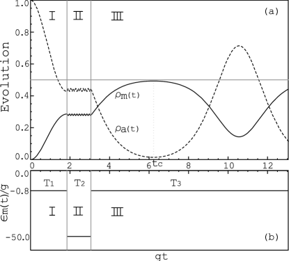
Figure 2: (a) Time-dependence of the atomic and molecular populations. (b) Schematic time-dependence of $\epsilon_{\mathrm{m}}(t)$ under the sequence of magnetic field pulses. The horizontal line in (a) indicates the limit of the complete conversion of molecules, ${\it i.e.}$, $\rho_{\mathrm{m}}=1/2$. The two vertical lines separate the evolution process into three regions (I, II, and III) corresponding to the time-dependent magnetic field pulses. Durations of each region is denoted by $T_{i}$ ($i=1$, 2, and 3).

Let us discuss the evolution of the system initiated from the pure atomic state. As shown in Fig. 2, the two magnetic field pulses correspond to $\epsilon_{\mathrm{m}}(t)/g=-0.8$ when $0\leq t<T_{1}$ and $(T_{1}+T_{2})\leq t\leq(T_{1}+T_{2}+T_{3})$. From Fig. 1(a) and 1(c) we can find that, the Rabi oscillation period is $gT_{\mathrm{Rabi}}\simeq 3.7$ if only the first magnetic field pulse exists. Thus in Fig. 2 we choose $T_{1}=T_{\mathrm{Rabi}}/2$ in order to reach the maximum of the molecular conversion at the end of the first magnetic field pulse, which is about $\rho_{\mathrm{m}}\simeq 0.27$. During $T_{1}\leq t<(T_{1}+T_{2})$ the smallness of $\epsilon_{\mathrm{m}}(t)$ is accompanied with a fast oscillation of small amplitude during the evolution. In our simulation $gT_{2}=1.21$ during which the system has already oscillated for dozens of periods. This specific value of $T_{2}$ is chosen to make sure that, when $t\geq(T_{1}+T_{2})$ the system undergoes a slow Rabi oscillation of large amplitude (obeying energy conservation) whose maximum value can get close to the limit of a complete conversion, ${\it i.e.}$, $\rho_{\mathrm{m}}=1/2$. This would never happen if one just had applied one magnetic field pulse, which is illustrated in Fig. 1(a). In our simulation the maximum conversion efficiency locates at $gt_{\mathrm{c}}\simeq 6.25$ with $\rho_{\mathrm{m}}(t_{\mathrm{c}})\simeq 0.49$.

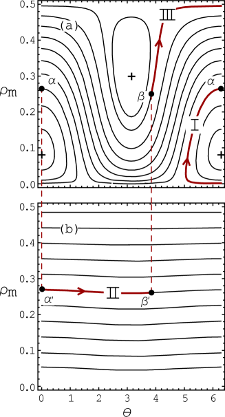
Figure 3: (Color online) Energy contour for (a) $\epsilon_{\mathrm{m}}/g=-0.8$ and (b) $\epsilon_{\mathrm{m}}/g=-50$ in the phase space of $\rho_{\mathrm{m}}$ and $\theta$. The arrows show the evolution direction. The extreme points (marked by the plus sign) correspond to the fixed point solutions discussed in Sec. III. $\rho_{\mathrm{m}}=1/2$ is unmarked due to the not well-defined $\theta$. Note that $\alpha$ ($\beta$) and $\alpha^{\prime}$ ($\beta^{\prime}$) refer to the same point in the phase space.

Now we interpret this evolution behavior with the help of the energy contour of Eq. (5) in the phase space of $\rho_{\mathrm{m}}$ and $\theta$. Figure. 3(a) corresponds to $\epsilon_{\mathrm{m}}/g=-0.8$ while 3(b) corresponds to $\epsilon_{\mathrm{m}}/g=-50.0$. The different values of $\epsilon_{\mathrm{m}}$ yield different energy contour patterns. Here the energy conservation plays the major role.

During the first magnetic field pulse (I), $0\leq t<T_{1}$, the system oscillates in the Rabi type obeying the energy conservation law. In our simulation, the undefined $\theta(0)$ at the beginning of the evolution is chosen to be zero as shown in Figure. 3(a). At $t=T_{1}=T_{\mathrm{Rabi}}/2$, the sudden change of magnetic field switches the energy landscape described by the contour pattern in Fig. 3(a) to that in Fig. 3(b) while keeping the instantaneous location in the phase space unchanged ($\alpha^{\prime}$ corresponding to $\alpha$) at the moment. Note that the system energy is changed during this switch. In contrast, during the sequential magnetic field (II) which is far away from the resonance, energy conservation still holds, forcing the system to evolve with a fast oscillation of small amplitude. Suppose at $t=(T_{1}+T_{2})$ it evolves to the location $\beta^{\prime}$ given in Fig. 3(b). When the magnetic field is switched back to the original value of the first pulse at the same moment, the system locates at a new position $\beta$ (corresponding to $\beta^{\prime}$) which is no longer inside the original trajectory of the Rabi oscillation induced by the first pulse. Consequently, the system has entered another trajectory with constant energy. Furthermore, the energy conservation will definitely bring the system close to a complete conversion into molecules (III). Note that the evolution direction in Figure. 3 can be determined by analyzing Eqs. (2) and (3).

V Summary And Discussion

We considered the atom-to-molecule conversion near a Feshbach resonance and proposed a strategy to enhance the conversion efficiency. In the mean-field approximation, we derived the classical Hamiltonian and the corresponding evolution equations, together with the fixed point solutions of the classical system. Starting from the pure atomic condensate, we investigated the Rabi oscillation and presented the analytical expression for the oscillation period versus $\epsilon_{\mathrm{m}}/g$. In analogy with Ramsey experiments, we applied to the system a sequence of magnetic field pulses. We found that, by tuning the durations of each pulse and the evolution time elaborately, it is possible to approach a complete conversion that can never be achieved by a single pulse. With the help of the energy contour in the phase space of $\rho_{\mathrm{m}}$ and $\theta$, we gave a simple interpretation of such evolution based on the energy conservation law.

The advantage of our proposal lies in the fact that it does not require the magnetic field to cross or closely approach the Feshbach resonance, which can avoid the substantial system heating and particle loss induced by the enhanced interactions. In our proposal the magnetic field in each pulse (we denote it by $B_{\mathrm{p}}$) could take values away from $B_{0}$. Thus, we can achieve much higher ultimate phase space densities ($n\lambda_{\mathrm{th}}^{3}$ with $\lambda_{\mathrm{th}}$ being the thermal de Broglie wavelength) and hence higher possible conversion efficiencies. In our simulation, the magnitudes $B_{\mathrm{p}}$ of the two pulses are taken to be the same, but they can also be different to obtain a higher conversion efficiency. However, as $|B_{\mathrm{p}}-B_{0}|$ increases, the value of $\epsilon_{\mathrm{m}}$ decreases accordingly, which may lead to the suppression of the amplitude of Rabi oscillation during the two magnetic field pulses. The value of $B_{\mathrm{p}}$ should not to be too far away from $B_{0}$. For example, the analysis of Fig. 3, together with the fixed point solutions in Table 1 suggest that the optimal range of $B_{\mathrm{p}}$ can be chosen such that $-\sqrt{2}\lesssim\epsilon_{\mathrm{m}}/g\lesssim 0$.

The fast ramps of magnetic field pulses may result in the loss of atoms and the production of an additional component which is considered as an atomic burst consisting of correlated pairs with a comparatively high relative velocity FR Ramsey Donley . To take this effect into account, our model should be extended to include the atomic burst as a new component of continuum spectrum. This may bring about the damping in the Rabi oscillation Continuum Javanainen , but the effects of the atomic burst would decrease as the temperature drops close to zero.

The work is supported by NSFC Grant No. 10674117, No. 10874149 and partially by PCSIRT Grant No. IRT0754.

References

- (1) C. A. Regal, M. Greiner, and D. S. Jin, Phys. Rev. Lett. 92, 040403 (2004).
- (2) R. V. Krems, Int. Rev. Phys. Chem. 24, 99 (2005).
- (3) D. W. Rein, J. Mol. Evol. 4, 15 (1974).
- (4) V. S. Letokhov, Phys. Lett. A 53, 275 (1975).
- (5) V. V. Flambaum and M. G. Kozlov, Phys. Rev. Lett. 99, 150801 (2007).
- (6) D. DeMille, F. Bay, S. Bickman, D. Kawall, D. Krause, Jr., S. E. Maxwell, and L. R. Hunter, Phys. Rev. A 61, 052507 (2000).
- (7) J. J. Hudson, B. E. Sauer, M. R. Tarbutt, and E. A. Hinds, Phys. Rev. Lett. 89, 023003 (2002).
- (8) H. Feshbach, Ann. Phys. (N.Y.) 19, 287 (1962).
- (9) S. L. Cornish, N. R. Claussen, J. L. Roberts, E. A. Cornell, and C. E. Wieman, Phys. Rev. Lett. 85, 1795 (2000).
- (10) C. A. Regal, C. Ticknor, J. L. Bohn, and D. S. Jin, Nature (London) 424, 47 (2003).
- (11) K. E. Strecker, G. B. Partridge, and R. G. Hulet, Phys. Rev. Lett. 91, 080406 (2003).
- (12) J. Herbig, T. Kraemer, M. Mark, T. Weber, C. Chin, H. C. Nägerl, and R. Grimm, Science 301, 1510 (2003).
- (13) K. Xu, T. Mukaiyama, J. R. Abo-Shaeer, J. K. Chin, D. E. Miller, and W. Ketterle, Phys. Rev. Lett. 91, 210402 (2003).
- (14) S. Du rr, T. Volz, A. Marte, and G. Rempe, Phys. Rev. Lett. 92, 020406 (2004).
- (15) M. Mark, T. Kraemer, J. Herbig, C. Chin, H. C. Nägerl, and R. Grimm, Europhys. Lett. 69, 706 (2005).
- (16) E. Hodby, S. T. Thompson, C. A. Regal, M. Greiner, A. C. Wilson, D. S. Jin, E. A. Cornell, and C. E. Wieman, Phys. Rev. Lett. 94, 120402 (2005).
- (17) S. T. Thompson, E. Hodby, and C. E. Wieman, Phys. Rev. Lett. 95, 190404 (2005)
- (18) C. Weber, G. Barontini, J. Catani, G. Thalhammer, M. Inguscio, and F. Minardi, Phys. Rev. A 78, 061601(R) (2008)
- (19) J. Cubizolles, T. Bourdel, S. J. J. M. F. Kokkelmans, G. V. Shlyapnikov, and C. Salomon, Phys. Rev. Lett. 91, 240401 (2003).
- (20) A. N. Nikolov, E. E. Eyler, X. T. Wang, J. Li, H. Wang, W. C. Stwalley, and P. L. Gould, Phys. Rev. Lett. 82, 703 (1999).
- (21) A. Fioretti, D. Comparat, A. Crubellier, O. Dulieu, F. Masnou-Seeuws, and P. Pillet, Phys. Rev. Lett. 80, 4402 (1998).
- (22) T. Takekoshi, B. M. Patterson, and R. J. Knize, Phys. Rev. A 59, R5 (1999).
- (23) R. Wynar, R. S. Freeland, D. J. Han, C. Ryu, and D. J. Heinzen, Science 287, 1016 (2000).
- (24) E. A. Shapiro, M. Shapiro, A. Pe’er, and J. Ye, Phys. Rev. A 75, 013405 (2007).
- (25) L. H. Lu and Y. Q. Li, Phys. Rev. A 76, 053608 (2007)
- (26) E. A. Donley, N. R. Claussen, S. T. Thompson, and C. E. Wieman, Nature (London) 417, 529 (2002).
- (27) X. Q. Xu, L. H. Lu, and Y. Q. Li, Phys. Rev. A 78, 043609 (2008).
- (28) J. Javanainen and M. Mackie, Phys. Rev. Lett. 88, 090403 (2002).