On the lower bound on the exchange-correlation energy in two dimensions

Abstract

We study the properties of the lower bound on the exchange-correlation energy in two dimensions. First we review the derivation of the bound and show how it can be written in a simple density-functional form. This form allows an explicit determination of the prefactor of the bound and testing its tightness. Next we focus on finite two-dimensional systems and examine how their distance from the bound depends on the system geometry. The results for the high-density limit suggest that a finite system that comes as close as possible to the ultimate bound on the exchange-correlation energy has circular geometry and a weak confining potential with a negative curvature.

1 Introduction

The lower bound on the quantum mechanical part of the Coulomb interaction energy, commonly known as the Lieb-Oxford (LO) bound [1], is a key concept in many-body physics. The bound is not only of fundamental importance for, e.g., analyzing the stability of matter [2], but it has also been used as a key constraint in the construction of several exchange-correlation functionals within density-functional theory (DFT), which is a standard tool in electronic-structure calculations of atoms, molecules, solids, and various nanoscale systems [3]. Recently, substantial efforts have been directed at testing the tightness of the original three-dimensional LO bound [4, 5] and in finding tighter forms [6, 7].

In view of the growing interest in two-dimensional (2D) systems, the existence and properties of the 2D form of the lower bound on the exchange-correlation energy are of immediate relevance. In this paper we review the known form of the 2D bound and show how it can be derived from scaling relations. We discuss the tight prefactor for the bound obtained from the properties of the homogeneous 2D electron gas (2DEG) in the low-density limit. We test this bound for finite 2D systems, and, in particular, by varying the shape of the system for a simple two-electron system, we propose a set of general properties for a finite 2D system which is as close as possible to the lower bound on the exchange-correlation energy.

2 Two-dimensional bound

Lieb, Solojev, and Yngvason [8] (LSY) have rigorously derived a 2D form of the LO bound, which can be expressed in terms of the indirect part of the interaction energy:

$$W_{xc}[\Psi]\equiv\left<\Psi|{\hat{V}}_{ee}|\Psi\right>-U[n]\geq-\,C\int d^{2}r\,n^{3/2}({\bf r}),$$ (1)

where ${\hat{V}}_{ee}=\sum_{i>j}|{\bf r}_{i}-{\bf r}_{j}|^{-1}$ is the Coulombic e-e interaction operator, $\Psi(\mathbf{r}_{1},...,\mathbf{r}_{N})$ is any normalized 2D many-body wave function, $n(\mathbf{r})$ is the corresponding density, and $U[n]$ is the classical Hartree energy. For the prefactor LSY estimated $C\leq C_{\rm LSY}=192\sqrt{2\pi}\approx 481$.

Interestingly, the exponent $3/2$ in Eq. (1) follows directly from universal scaling properties of the e-e interaction [7]. Under homogeneous 2D coordinate scaling, ${\bf r}\to\gamma{\bf r}$ ($0<\gamma<\infty$) [9] the $(2N)$-dimensional many-body wavefunction scales as $\Psi({\bf r}_{1}\ldots{\bf r}_{N})\rightarrow\Psi_{\gamma}({\bf r}_{1}\ldots{\bf r}_{N})=\gamma^{2N/2}\Psi(\gamma{\bf r}_{1}\ldots\gamma{\bf r}_{N})$, preserving normalization. This produces the number-conserving scaled density $n({\bf r})\to n_{\gamma}({\bf r})=\gamma^{2}n(\gamma{\bf r})$. Further, $W_{xc}[\Psi]\rightarrow W_{xc}[\Psi_{\gamma}]=\gamma W_{xc}[\Psi]$, since both the Coulomb interaction and its Hartree approximation scale linearly. Denoting the exponent in Eq. (1) by $\chi$, we then find the relation

$$\gamma W_{xc}[\Psi]\geq-\,C\,\gamma^{2(\chi-1)}\int d^{2}r\,n^{\chi}({\bf r}),$$ (2)

so that consistency with Eq. (1) gives $\chi=3/2$.

It was also conjectured in Ref. [7] by the present authors that the prefactor can be decreased to $C=1.96$ which corresponds to a significant tightening of the original 2D bound with $C_{\rm LSY}\approx 481$. The tightest bound, i.e., the lowest exchange-correlation energy corresponds to the 2DEG in the low-density limit, and hence all other 2D systems (including all real, finite systems) are energetically above this bound. However, it remains to be examined which type of a finite system is closest to the bound.

3 Density-functional form of the bound

Here we reformulate the bound in Eq. (1) in terms of density functionals. The right-hand side can be written in terms of the expression of the local-density approximation (LDA) for the electronic exchange in 2D,

$$E_{x}^{\rm LDA}[n]=-A\,\int d^{2}r\,n^{3/2}({\bf r}),$$ (3)

where $A=4\sqrt{2}/(3\sqrt{\pi})$. This formula has the same scaling with respect to the density as Eq. (1). Note that Eq. (3) is exact for the exchange energy of the 2DEG (constant $n$) by construction [10]. The left hand side of Eq. (1) can be written in terms of the exchange-correlation energy as defined in DFT, i.e., $E_{xc}[n]\equiv W_{xc}[n]+T_{c}[n]\geq W_{xc}[n]$, where $T_{c}$ is the difference between the many-body kinetic energy and the (single-particle) Kohn-Sham kinetic energy and it is always positive. Now, Eq. (1) becomes

$$E_{xc}[n]\geq\frac{C}{A}\;E_{x}^{\rm LDA}[n].$$ (4)

For any 2D system, we can now consider the density functional

$$\lambda[n]=\frac{E_{xc}[n]}{E_{x}^{\rm LDA}[n]}\leq\frac{C}{A}$$ (5)

with $E_{xc}[n]=E_{x}[n]+E_{c}[n]$. As mentioned above, the tightest 2D bound corresponds to the 2DEG in the low-density limit which yields the maximum value of Eq. (5), i.e., $\lambda_{\rm 2DEG}[r_{s}\rightarrow\infty]=1.84$, where $r_{s}=1/\sqrt{\pi n}$ is the density parameter in 2D.

4 Testing the bound

4.1 General remarks

In practice, calculation of $\lambda[n]$ for finite systems and thus testing the bound is seriously limited by the lack of reference data for exact exchange-correlation energies and exact densities. An exception is the 2D Hooke’s atom, i.e., a parabolic (harmonic) quantum dot (QD) with two electrons ($N=2$), for which analytic solutions are known [11], and which yields $\lambda[n]\approx 1.55$ as the maximum value [7].

It is also possible to approximate $\lambda$ from the exact reference data solely for the total energy $E_{\rm tot}$. This requires exact-exchange (EXX) or Hartree-Fock calculations to obtain the exchange energy, which, for closed-shell systems, can be written as

$$E_{x}[n]=-\int d^{2}r\int d^{2}r^{\prime}\,\frac{\left|\sum_{i=1}^{N/2}\psi_{i}^{*}({\bf r})\psi_{i}({\bf r}^{\prime})\right|^{2}}{|{\bf r}-{\bf r}^{\prime}|},$$ (6)

where $\psi_{i}$ are Kohn-Sham (or Hartree-Fock) orbitals. The correlation energy is then obtained as $E_{c}=E_{\rm tot}-E^{\rm EXX}_{\rm tot}$. It should be noted that Eq. (5) becomes now an approximation due to using both exact densities and EXX densities as the input instead of consistently using only the exact densities. Nevertheless, tests for few-electron parabolic and square-shaped QDs based on this strategy have led to values in the range $1.1\lesssim\lambda[n]\lesssim 1.5$ (Ref. [7]). The results for QDs suggest that the largest value for $\lambda$ is obtained with $N=2$.

4.2 Effects of geometry

To consistently analyze the dependence of $\lambda[n]$ on the system geometry, we focus in the following solely on the limit $r_{s}\rightarrow 0$. This corresponds to the noninteracting situation, since the kinetic energy scales as $r_{s}^{-2}$ and the interaction energy as $r_{s}^{-1}$ (cf. the opposite limit where interactions dominate and lead to Wigner crystallization [12]). Now, the correlation energy is zero, but Eq. (5) is still a well-defined quantity having a form

$$\lambda[r_{s}\rightarrow 0]=\frac{E_{x}[n]}{E_{x}^{\rm LDA}[n]}.$$ (7)

Furthermore, we set $N=2$ so that the exact exchange energy in Eq. (6) can be calculated as a simple integral over the density; in fact it is exactly minus half of the Hartree energy. To find the density we solve the Schrödinger equation for a noninteracting singlet state in the presence of an external confining potential $V(x,y)$. In the numerical procedure we use the octopus code [13]. Note that upon the condition that the potential scales homogenously with respect to the scaling parameter $\gamma$ (see above), we can choose any prefactor in the potential, i.e., any $\zeta$ in $\zeta V(x,y)$, in order to mimic the true interacting calculation in the limit $r_{s}\rightarrow 0$ corresponding to $n\rightarrow\infty$. This can be seen by considering $V(r)$ in the radial Schrödinger equation for $N=2$, where $\psi_{i}(r)\propto\sqrt{n(r)}$ ($i=1,2$). The form of the equation under uniform coordinate scaling ${\bf r}\to\gamma{\bf r}$ (see above) shows that $V(r)\rightarrow\gamma^{2}V(\gamma r)=\gamma^{2+\alpha}V(r)$, assuming that $V(r)$ scales homogenously with $\gamma$. Hence, a value for $\gamma$ can be found for any prefactor $\zeta$. In other words, changing the prefactor is equivalent to scaling of the density. And in fact, this is the case in all potentials given below, as all of them scale homogeneously with respect to $\gamma$. Moreover, Eq. (7) is now independent of $\gamma$.

First we consider a circular QD defined by a confining potential of the form

$$V_{\rm circular}(r)=|r|^{\alpha},$$ (8)

and a square-shaped QD defined by

$$V_{\rm square}(x,y)=|x|^{\alpha}+|y|^{\alpha}.$$ (9)

Here the parameter $\alpha$ determines the “steepness” of the potential.

Figure 1

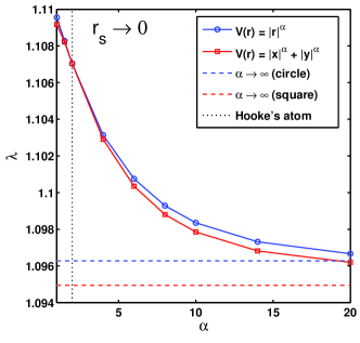
Figure 1: (color online) Values for $\lambda$ in two-electron quantum dots with varying external confining potential in the noninteracting limit.

shows $\lambda$ in the $r_{s}\rightarrow 0$ limit as a function of $\alpha$. Obviously, the two potentials are the same when $\alpha=2$, when they actually correspond to the 2D Hooke’s atom (dotted line) with $\lambda\approx 1.107$. At $\alpha>2$ we find monotonous decrease of $\lambda$, and the limit $\alpha\rightarrow\infty$, which corresponds to the hard-wall case, leads to $\lambda\approx 1.0963$ and $1.0949$ in circular and square QDs, respectively. Overall, the circular potential gives higher values of $\lambda$ than the square one.

Interestingly, the highest values for $\lambda$ are obtained at $\alpha<2$. In this regime, $\alpha=1$ corresponds to a cone (pyramid) in a circular (square) QD. The numerical accuracy of our eigenvalue solver limits the investigation to $\alpha=0.5$, which actually yields the largest $\lambda$ as seen in Fig. 1. Therefore, we assume that the maximum value for $\lambda$ could be found in a circular QD at $\alpha<0.5$, when the curvature is negative, i.e., $d^{2}V(r)/(dr^{2})<0$.

In Fig. 2

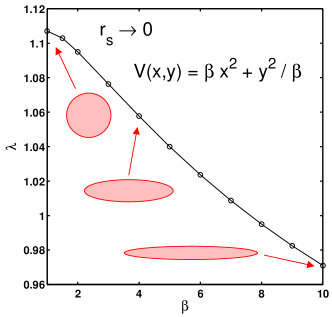
Figure 2: (color online) Values for $\lambda$ in elliptic quantum dots in the noninteracting limit. The shaded figures represent schematically the symmetry of the confining potentials.

we consider the $r_{s}\rightarrow 0$ limit in an elliptic confinement,

$$V_{\rm elliptic}(x,y)=\beta x^{2}+y^{2}/\beta,$$ (10)

where $\beta$ is related to the eccentricity, although this is not a formal definition. Similar confinement has been used in the QD studies in Refs. [14] and [15]. We find that $\lambda$ decreases as a function of $\beta$, and the highest value can be obtained in a parabolic system at $\beta=1$ (Hooke’s atom).

5 Conclusions and outlook

Summarizing the results reported in the previous section for finite systems, we have found that in order to find a maximum value of $\lambda$ in the $r_{s}\rightarrow 0$ limit, the confinement potential should be (i) circular instead of square or elliptic, and (ii) it should have a negative curvature. Assuming that these geometric effects carry over to $r_{s}>0$, and in particular to values for $r_{s}$ maximizing $\lambda(r_{s})$, and combining these findings with previous results for harmonic systems with $N\geq 1$ and $r_{s}>0$ (Ref. [7]), we advance the following conjecture: The maximum value of $\lambda$ in finite 2D systems, and hence the closest possible value to the ultimate bound on the exchange-correlation energy can be obtained in a two-particle system having circular symmetry and a weak confining potential with a negative curvature.

Similar to what was previously observed in 3D [4, 5, 6], smaller particle numbers in 2D produce larger values of the functional $\lambda[n]$ (Ref. [7]). This should be compared with the behavior of the function $\lambda(N)$, which for any $N$ produces an upper limit on $\lambda[n]$ for all densities integrating to this $N$. In 3D, $\lambda(N)$ is known rigorously [1, 4] to be monotonically increasing with $N$. We expect this to be true also in 2D, but have not proved it. In any case, the fact that the upper limit $\lambda(N)$ increases with $N$, while the actual value $\lambda[n]$ decreases is not a contradiction. It simply means that the LO bound becomes more and more generous as $N$ increases, and, conversely, tighter and tighter as $N$ decreases.

Overall, we conclude from the investigation of the present paper that, qualitatively and even semi-quantitatively, 2D systems behave similarly to 3D systems with respect to the appropriate LO bound.

Furthermore, in view of the results for the 2DEG and 2D Hooke’s atom [7] we may assume that a finite system with the largest $\lambda$ would have rather uniform density (except at the boundaries), and $\lambda$ would be very close to the bound value $\lambda_{\rm 2DEG}=1.84$. Although we cannot rigorously prove these assumptions for the potential or for the density at large $r_{s}$, we hope that these results will encourage similar geometric studies on finite systems where correlations are incorporated. This would require using, e.g., the density-functional formalism for strictly correlated electrons [16], or an inversion scheme [17], to reconstruct the exact external potential and the corresponding many-body problem for a given density.

This work was supported by the Academy of Finland, Deutsche Forschungsgemeinschaft, and the EU’s Sixth Framework Programme through the ETSF e-I3. In addition, C. R. P. was supported by EC’s Marie Curie IIF (MIF1-CT-2006-040222) and K. C. by FAPESP and CNPq.

References

- [1] E. H. Lieb and S. Oxford, Int. J. Quantum Chem. 19 (1981) 427.
- [2] L. Spruch, Rev. Mod. Phys. 63 (1991) 151.
- [3] For a review, see, e.g., R. M. Dreizler and E. K. U. Gross, Density functional theory (Springer, Berlin, 1990).
- [4] M. M. Odashima and K. Capelle, J. Chem. Phys. 127 (2007) 054106.
- [5] M. M. Odashima and K. Capelle, Int. J. Quantum Chem. 108 (2008) 2428.
- [6] M. M. Odashima, S. B. Trickey and K. Capelle, J. Chem. Theory Comput. 5 (2009) 798.
- [7] E. Räsänen, S. Pittalis, K. Capelle, and C. R. Proetto, Phys. Rev. Lett. 102 (2009) 206406.
- [8] E. H. Lieb, J. P. Solovej, and J. Yngvason, Phys. Rev. B 51 (1995) 10646.
- [9] M. Levy and J. P. Perdew, Phys. Rev. B 48 (1993) 11638.
- [10] A. K. Rajagopal and J. C. Kimball, Phys. Rev. B 15 (1977) 2819.
- [11] M. Taut, J. Phys. A 27 (1994) 1045.
- [12] E. P. Wigner, Phys. Rev. 46 (1934) 1002.
- [13] M. A. L. Marques, A. Castro, G. F. Bertsch, A. Rubio, Comput. Phys. Commun. 151 (2003) 60; A. Castro, H. Appel, M. Oliveira, C. A. Rozzi, X. Andrade, F. Lorenzen, M. A. L. Marques, E. K. U. Gross, and A. Rubio, Phys. Stat. Sol. (b) 243 (2006) 2465.
- [14] D. G. Austing, S. Sasaki, S. Tarucha, S. M. Reimann, M. Koskinen, and M. Manninen, Phys. Rev. B 60 (1999) 11514.
- [15] H. Saarikoski, S. M. Reimann, E. Räsänen, A. Harju, and M. J. Puska, Phys. Rev. B 71 (2005) 035421.
- [16] P. Gori-Giorgi, M. Seidl, and G. Vignale, Phys. Rev. Lett. 103 (2009) 166402.
- [17] J. P. Coe, K. Capelle, and I. D’Amico, Phys. Rev. A 79 (2009) 032504.