Towards the Albertson conjecture

Abstract.

Albertson conjectured that if a graph $G$ has chromatic number $r$ then its crossing number is at least as much as the crossing number of $K_{r}$. Albertson, Cranston, and Fox verified the conjecture for $r\leq 12$. We prove the statement for $r\leq 16$.

Dedicated to the memory of Michael O. Albertson.

1. Introduction

Graphs in this paper are without loops and multiple edges. Every planar graph is four-colorable by the Four Color Theorem [2, 23]. Efforts to solve the Four Color Problem had a great effect on the development of graph theory, and it is one of the most important theorems of the field.

The crossing number ${\mbox{\sc cr}}(G)$ of a graph $G$ is the minimum number of edge crossings in a drawing of $G$ in the plane. It is a natural relaxation of planarity, see [24] for a survey. The chromatic number $\chi(G)$ of a graph $G$ is the minimum number of colors in a proper coloring of $G$. The Four Color Theorem states if ${\mbox{\sc cr}}(G)=0$ then $\chi(G)\leq 4$. Oporowski and Zhao [18] proved that every graph with crossing number at most two is 5-colorable. Albertson et al. [5] showed that if ${\mbox{\sc cr}}(G)\leq 6$, then $\chi(G)\leq 6$. It was observed by Schaefer that if ${\mbox{\sc cr}}(G)=k$ then $\chi(G)=O(\sqrt[4]{k})$ and this bound cannot be improved asymptotically [4].

It is well-known that graphs with chromatic number $r$ do not necessarily contain $K_{r}$ as a subgraph, they can have clique number 2 [26]. The Hajós conjecture proposed that graphs with chromatic number $r$ contain a subdivision of $K_{r}$. This conjecture, whose origin is unclear but attributed to Hajós, turned out to be false for $r\geq 7$. Moreover, it was shown by Erdős and Fajtlowicz [9] that almost all graphs are counterexamples. Albertson conjectured the following.

Conjecture 1.

If $\chi(G)=r$, then ${\mbox{\sc cr}}(G)\geq{\mbox{\sc cr}}(K_{r})$.

This statement is weaker than Hajós’ conjecture, since if $G$ contains a subdivision of $K_{r}$ then ${\mbox{\sc cr}}(G)\geq{\mbox{\sc cr}}(K_{r})$.

For $r=5$, Albertson’s conjecture is equivalent to the Four Color Theorem. Oporowski and Zhao [18] verified it for $r=6$, Albertson, Cranston, and Fox [4] proved it for $r\leq 12$. In this note we take one more little step.

Theorem 2.

For $r\leq 16$, if $\chi(G)=r$, then ${\mbox{\sc cr}}(G)\geq{\mbox{\sc cr}}(K_{r})$.

In their proof, Albertson, Cranston, and Fox combined lower bounds for the number of edges of $r$-critical graphs, and lower bounds on the crossing number of graphs with given number of vertices and edges. Our proof is very similar, but we use better lower bounds in both cases.

Albertson, Cranston, and Fox proved that any minimal counterexample to Albertson’s conjecture should have less than $4r$ vertices. We slightly improve this result as follows.

Lemma 3.

If $G$ is an $r$-critical graph with $n\geq 3.57r$ vertices, then ${\mbox{\sc cr}}(G)\geq{\mbox{\sc cr}}(K_{r})$.

In Section 2 we review lower bounds for the number of edges of $r$-critical graphs, in Section 3 we discuss lower bounds on the crossing number, and in Section 4 we combine these bounds to obtain the proof of Theorem 2. In Section 5 we prove Lemma 3.

The letter $n$ always denotes the number of vertices of $G$. In notation and terminology we follow Bondy and Murty [6]. In particular, the join of two disjoint graphs $G$ and $H$ arises by adding all edges between vertices of $G$ and $H$. It is denoted by $G\vee H$. A vertex $v$ is called simplicial if it has degree $n-1$. If a graph $G$ contains a subdivision of $H$, then we also say that $G$ contains a topological $H$. A vertex $v$ is adjacent to a vertex set $X$ means that each vertex of $X$ is adjacent to $v$.

2. Color-critical graphs

Around 1950, Dirac introduced the concept of color criticality in order to simplify graph coloring theory, and it has since led to many beautiful theorems. A graph $G$ is $r$-critical if $\chi(G)=r$ but all proper subgraphs of $G$ have chromatic number less than $r$. In what follows, let $G$ denote an $r$-critical graph with $n$ vertices and $m$ edges.

Since $G$ is $r$-critical, every vertex has degree at least $r-1$ and therefore,
$2m\geq(r-1)n$. Dirac [7] proved that for $r\geq 3$, if $G$ is not complete, then $2m\geq(r-1)n+(r-3)$. For $r\geq 4$, Dirac [8] gave a characterization of $r$-critical graphs with excess $r-3$. For any fixed $r\geq 3$ let $\Delta_{r}$ be the family of graphs $G$ whose vertex set consists of three non-empty, pairwise disjoint sets $A,B_{1},B_{2}$ with $|B_{1}|+|B_{2}|=|A|+1=r-1$ and two additional vertices $a$ and $b$ such that $A$ and $B_{1}\cup B_{2}$ both span cliques in $G$, they are not connected by any edge, $a$ is connected to $A\cup B_{1}$ and $b$ is connected to $A\cup B_{2}$. See Figure 1. Graphs in $\Delta_{r}$ are called Hajós graphs of order $2r-1$. Observe that that these graphs have chromatic number $r$ and they contain a topological $K_{r}$, hence they satisfy Hajós’ conjecture.

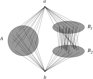
Figure 1. The family $\Delta_{r}$

Gallai [10] proved that $r$-critical graphs with at most $2r-2$ vertices are the join of two smaller graphs, i.e. their complement is disconnected. Based on this observation, he proved that non-complete $r$-critical graphs on at most $2r-2$ vertices have much larger excess than in Dirac’s result.

Lemma 4.

[10] Let $r,p$ be integers satisfying $r\geq 4$ and $2\leq p\leq r-1$. If $G$ is an $r$-critical graph with $n=r+p$ vertices, then $2m\geq(r-1)n+p(r-p)-2$, where equality holds if and only if $G$ is the join of $K_{r-p-1}$ and $G\in\Delta_{p+1}$.

Since every $G\in\Delta_{p+1}$ contains a topological $K_{p+1}$, the join of $K_{r-p-1}$ and $G$ contains a topological $K_{r}$. This yields a slight improvement for our purposes.

Corollary 5.

Let $r,p$ be integers satisfying $r\geq 4$ and $2\leq p\leq r-1$. If $G$ is an $r$-critical graph with $n=r+p$ vertices, and $G$ does not contain a topological $K_{r}$, then $2m\geq(r-1)n+p(r-p)-1$.

We call the bound given by Corollary 5 the Gallai bound.

For $r\geq 3$, let ${\mathcal{E}}_{r}$ denote the family of graphs G, whose vertex set consists of four non-empty pairwise disjoint sets $A_{1},A_{2},B_{1},B_{2}$, where $|B_{1}|+|B_{2}|=|A_{1}|+|A_{2}|=r-1$ and $|A_{2}|+|B_{2}|\leq r-1$, and one additional vertex $c$ such that $A=A_{1}\cup A_{2}$ and $B=B_{1}\cup B_{2}$ are cliques in $G$, $N_{G}(c)=A_{1}\cup B_{1}$ and a vertex $a\in A$ is adjacent to a vertex $b\in B$ if and only if $a\in A_{2}$ and $b\in B_{2}$.

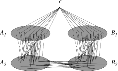
Figure 2. The family ${\mathcal{E}}_{r}$

Clearly ${\mathcal{E}}_{r}\supset\Delta_{r}$, and every graph $G\in{\mathcal{E}}_{r}$ is $r$-critical with $2r-1$ vertices. Kostochka and Stiebitz [15] improved the bound of Dirac as follows.

Lemma 6.

[15] Let $r\geq 4$ and $G$ be an $r$-critical graph. If $G$ is neither $K_{r}$ nor a member of ${\mathcal{E}}_{r}$, then $2m\geq(r-1)n+(2r-6)$.

It is not difficult to prove that any member of ${\mathcal{E}}_{r}$ contains a topological $K_{r}$. Indeed, $A$ and $B$ both span a complete graph on $r-1$ vertices. We only have to show that vertex $c$ is connected to $A_{2}$ or $B_{2}$ by vertex-disjoint paths. To see this, we observe that $|A_{2}|$ or $|B_{2}|$ is the smallest of $\{|A_{1}|,|A_{2}|,|B_{1}|,|B_{2}|\}$. Indeed, if $|B_{1}|$ was the smallest, then $|A_{2}|>|B_{1}|$ and $|B_{2}|>|B_{1}|$ implies $|A_{2}|+|B_{2}|>|B_{1}|+|B_{2}|=r-1$ contradicting our assumption. We may assume that $|A_{2}|$ is the smallest. Now $c$ is adjacent to $A_{1}$, and there is a matching of size $|A_{2}|$ between $B_{1}$ and $B_{2}$ and between $B_{2}$ and $A_{2}$, respectively. That is, we can find a set $S$ of disjoint paths from $c$ to $A_{2}$. In this way $A\cup c\cup S$ is a topological $r$-clique.

Corollary 7.

Let $r\geq 4$ and $G$ be an $r$-critical graph. If $G$ does not contain a topological $K_{r}$ then $2m\geq(r-1)n+(2r-6)$.

Let us call this the Kostochka, Stiebitz bound, or KS-bound for short.

In what follows, we obtain a complete characterization of $r$-critical graphs on $r+3$ or $r+4$ vertices.

Lemma 8.

For $r\geq 8$, there are precisely two $r$-critical graphs on $r+3$ vertices. They can be constructed from two $4$-critical graphs on seven vertices by adding simplicial vertices.

Figure 3. The two $4$-critical graphs on seven vertices

Proof.

The proof is by induction on $r$. For the base case $r=8$, there are precisely two $8$-critical graphs on $11$ vertices, see Royle’s complete search [21].

Let $G$ be an $r$-critical graph with $r\geq 9$ and $n=r+3\geq 12$. We know that the minimum degree is at least $r-1=n-4$. If $G$ has a simplicial vertex $v$, then we use induction. So we may assume that every vertex in $\overline{G}$, the complement of $G$ has degree 1, 2 or 3. By Gallai’s theorem, $\overline{G}$ is disconnected. Observe the following: if there are at least four independent edges in $\overline{G}$, then $\chi(G)\leq n-4=r-1$, a contradiction. That is, there are at most three independent edges in $\overline{G}$. Therefore, $\overline{G}$ has two or three components. If there is a triangle in the complement, then we can save two colors. If there were two triangles, then $\chi(G)\leq n-4=r-1$, a contradiction.

Assume that there are three components in $\overline{G}$. Since each degree is at least one, there are at least three independent edges. Therefore, there is no triangle in $\overline{G}$ and no path with three edges. That is, the complement consists of three stars. Since the degree is at most three and there are at least $12$ vertices, there is only one possibility: $\overline{G}=K_{1,3}\cup K_{1,3}\cup K_{1,3}$, see Figure 4.

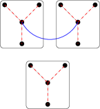
Figure 4. The complement and a removable edge

We have to check whether this concrete graph is indeed critical. We observe, that the edge connecting two centers of these stars is not critical, a contradiction.

In the remaining case, $\overline{G}$ has two components $H_{1}$ and $H_{2}$. Since there are at most three independent edges, there is one in $H_{1}$ and two in $H_{2}$. It implies that $H_{1}$ has at most four vertices. Therefore, $H_{2}$ has at least eight vertices. Consider a spanning tree $T$ of $H_{2}$ and remove two adjacent vertices of $T$, one of them being a leaf. It is easy to see that the remainder of $T$ contains a path with three edges. Therefore, in total we found three independent edges of $H_{2}$, a contradiction. ∎

We need the following result of Gallai.

Theorem 9.

[10] Let $r\geq 3$ and $n<\frac{5}{3}r$. Then every $r$-critical, $n$-vertex graph contains at least $\left\lceil\frac{3}{2}\left(\frac{5}{3}r-n\right)\right\rceil$ simplicial vertices.

Lemma 10.

For $r\geq 6$, there are precisely twenty-two $r$-critical graphs on $r+4$ vertices. They can be constructed by adding simplicial vertices to one of the following:a $3$-critical graph on seven vertices,
four $4$-critical graphs on eight vertices,
sixteen $5$-critical graphs on nine vertices, or
a $6$-critical graphs on ten vertices.

Proof.

For the base of induction, we use Royle’s table again, see [21]. The full computer search shows that there are precisely twenty-two $6$-critical graphs on ten vertices. For the induction step, we use Lemma 9 and see that there are at least $r-6$ simplicial vertices. Since $r\geq 7$, there is always a simplicial vertex. We remove it and use the induction hypothesis to finish the proof. ∎

There is an explicit list of twenty-one $5$-critical graphs on nine vertices [21]. We have checked, partly manually, partly using Mader’s extremal result [16], that each of those graphs contains a topological $K_{5}$. Also the above mentioned $6$-critical graph on ten vertices contains a topological $K_{6}$. These results imply the following

Corollary 11.

Any $r$-critical graph on at most $r+4$ vertices satisfy the Hajós conjecture.

We conjecture that the following slightly more general statement can be proved with similar methods.

Conjecture 12.

Let $G$ be an $r$-critical graph on $r+o(r)$ vertices. Then $G$ satisfies the Hajós conjecture.

3. The crossing number

It follows from Euler’s formula that a planar graph can have at most $3n-6$ edges. Suppose that $G$ has $m\geq 3n-6$ edges. By deleting crossing edges one by one, it follows by induction that for $n\geq 3$,

(1) $${\mbox{\sc cr}}(G)\geq m-3(n-2)$$

Pach et. al. [19] generalized it and proved the following lower bounds. Each one holds for any graph $G$ with $n\geq 3$ vertices and $m$ edges.

(2) $${\mbox{\sc cr}}(G)\geq 7m/3-25(n-2)/3$$

(3) $${\mbox{\sc cr}}(G)\geq 3m-35(n-2)/3$$

(4) $${\mbox{\sc cr}}(G)\geq 4m-103(n-2)/6$$

(5) $${\mbox{\sc cr}}(G)\geq 5m-25(n-2)$$

Inequality (1) is the best for $m\leq 4(n-1)$, (2) is the best for $4(n-2)\leq m\leq 5(n-2)$, (3) is the best for $5(n-2)\leq m\leq 5.5(n-2)$, (4) is the best for $5.5(n-2)\leq m\leq 47(n-2)/6$, and (5) is the best for $47(n-2)/6\leq m$.

It was also shown in [19] that (1) can not be improved in the range $m\leq 4(n-1)$,and (2) can not be improved in the range $4(n-2)\leq m\leq 5(n-2)$, apart from an additive constant. The other inequalities are conjectured to be far from optimal. Using the methods in [19] one can obtain an infinite family of such linear inequalities, of the form $am-b(n-2)$.

The most important inequality for crossing numbers is undoubtedly the Crossing Lemma, first proved by Ajtai, Chvátal, Newborn, Szemerédi [1], and independently by Leighton [13]. If $G$ has $n$ vertices and $m\geq 4n$ edges, then

(6) $${\mbox{\sc cr}}(G)\geq\frac{1}{64}\frac{m^{3}}{n^{2}}.$$

The original constant was much larger, the constant $\frac{1}{64}$ comes from the well-known probabilistic proof of Chazelle, Sharir, and Welzl [3]. The basic idea is to take a random spanned subgraph and apply inequality (1) for that.

The order of magnitude of this bound can not be improved, see [19], the best known constant is obtained in [19]. If $G$ has $n$ vertices and $m\geq\frac{103}{16}n$ edges, then

(7) $${\mbox{\sc cr}}(G)\geq\frac{1}{31.1}\frac{m^{3}}{n^{2}}.$$

The proof is very similar to the proof of (6), the main difference is that instead of (1), inequality (4) is applied for the random subgraph. The proof of the following technical lemma is based on the same idea.

Lemma 13.

Suppose that $n\geq 10$, and $0<p\leq 1$. Let

$${\mbox{\sc cr}}(n,m,p)=\frac{4m}{p^{2}}-\frac{103n}{6p^{3}}+\frac{103}{3p^{4}}-\frac{5n^{2}(1-p)^{n-2}}{p^{4}}.$$

Then for any graph $G$ with $n$ vertices and $m$ edges

$${\mbox{\sc cr}}(G)\geq{\mbox{\sc cr}}(n,m,p).$$

Proof.

Observe that inequality (4) does not hold for graphs with at most two vertices. For any graph $G$, let

$${\mbox{\sc cr}}^{\prime}(G)=\left\{\begin{array}[]{ll}{\mbox{\sc cr}}(G)&{\mbox{if }}n\geq 3\\ 4&{\mbox{if }}n=2\\ 18&{\mbox{if }}n=1\\ 35&{\mbox{if }}n=0\end{array}\right.$$

It is easy to see that for any graph $G$

(8) $${\mbox{\sc cr}}^{\prime}(G)\geq 4m-\frac{103}{6}(n-2).$$

Let $G$ be a graph with $n$ vertices and $m$ edges. Consider a drawing of $G$ with ${\mbox{\sc cr}}(G)$ crossings. Choose each vertex of $G$ independently with probability $p$, and let $G^{\prime}$ be a subgraph of $G$ spanned by the selected vertices. Consider the drawing of $G^{\prime}$ inherited from the drawing of $G$, that is, each edge of $G^{\prime}$ is drawn exactly as it is drawn in $G$. Let $n^{\prime}$ and $m^{\prime}$ be the number of vertices and edges of $G^{\prime}$, and let $x$ be the number of crossings in the present drawing of $G^{\prime}$. Using that $E(n^{\prime})=pn$, $E(m^{\prime})=p^{2}m$, $E(x)=p^{4}{\mbox{\sc cr}}(G)$, and the linearity of expectations,

$$E(x)\geq E({\mbox{\sc cr}}(G^{\prime}))\geq E({\mbox{\sc cr}}^{\prime}(G^{\prime}))-4P(n^{\prime}=2)-18P(n^{\prime}=1)-35P(n^{\prime}=0)\geq$$

$$\geq 4p^{2}m-\frac{103}{6}pn+\frac{103}{3}-4{n\choose 2}p^{2}(1-p)^{n-2}-18np(1-p)^{n-1}-35(1-p)^{n}\geq$$

$$\geq 4p^{2}m-\frac{103}{6}pn+\frac{103}{3}-5n^{2}(1-p)^{n-2}.$$

Dividing by $p^{4}$ we obtain the statement of the Lemma. ∎

Note that in our applications $p$ will be at least $1/2$, $n$ will be at least 13, therefore, the last term in the inequality, $\frac{5n^{2}(1-p)^{n-2}}{p^{4}}$, will be negligible.

We also need some bounds on the crossing number of the complete graph, ${\mbox{\sc cr}}(K_{r})$. It is not hard to see that

(9) $${\mbox{\sc cr}}(K_{r})\leq Z(r)=\frac{1}{4}\left\lfloor\frac{r}{2}\right\rfloor\left\lfloor\frac{r-1}{2}\right\rfloor\left\lfloor\frac{r-2}{2}\right\rfloor\left\lfloor\frac{r-3}{2}\right\rfloor,$$

see e. g. [22]. Guy conjectured [11] that ${\mbox{\sc cr}}(K_{r})=Z(r)$. This conjecture has been verified for $r\leq 12$ but still open for $r>12$. The best known lower bound is due to de Klerk et. al. [14]: ${\mbox{\sc cr}}(K_{r})\geq 0.86Z(r)$.

4. Proof of Theorem 2

Suppose that $G$ is an $r$-critical graph. If $G$ contains a topological $K_{r}$, then clearly ${\mbox{\sc cr}}(G)\geq{\mbox{\sc cr}}(K_{r})$. Suppose in the sequel that $G$ does not contain a topological $K_{r}$.

Therefore, we can apply the Kostochka, Stiebitz, and the Gallai bounds on the number of edges. Then we use Lemma 13 to get the desired lower bound on the crossing number. Albertson et. al. [4] used the same approach, but they used a weaker version of the Kostochka, Stiebitz, and the Gallai bounds, and instead of Lemma 13 they applied the weaker inequality (4). In the next table, we include the results of our calculations. For comparison, we also included the result Albertson et al. might have had using (4). In the Appendix we present our simple Maple program performing all calculations.

1. Let $r=13$. By (9) we have ${\mbox{\sc cr}}(K_{13})\leq 225$.

$n$	$e$	bound (4)	$p$	$\lceil{\mbox{\sc cr}}(n,m,p)\rceil$
18	128	238	0.719	288
19	135	249	0.732	296
20	141	255	0.751	298
21	146	258	0.774	294

If $n\geq 22$, then the KS-bound combined with (4) gives the desired result.
$2m\geq 12n+20\Rightarrow{\mbox{\sc cr}}(G)\geq 4(6n+10)-103/6(n-2)\geq 224.67$, if $n\geq 22$.

2. Let $r=14$. By (9) we have ${\mbox{\sc cr}}(K_{14})\leq 315$.

$n$	$e$	bound (4)	$p$	$\lceil{\mbox{\sc cr}}(n,m,p)\rceil$
19	146	293	0.659	388
20	154	307	0.670	402
21	161	318	0.684	407
22	167	325	0.702	406
23	172	328	0.723	398
24	176	327	0.747	384
25	179	322	0.775	366
26	181	312	0.807	344

If $n\geq 27$, then the KS-bound combined with (4) gives the desired result.
$2m\geq 13n+22\Rightarrow{\mbox{\sc cr}}(G)\geq 4(6.5n+11)-103/6(n-2)\geq 316$, if $n\geq 27$.

3. Let $r=15$. By (9) we have ${\mbox{\sc cr}}(K_{15})\leq 441$.

$n$	$e$	bound (4)	$p$	$\lceil{\mbox{\sc cr}}(n,m,p)\rceil$
20	165	351	0.610	510
21	174	370	0.617	531
22	182	385	0.623	542
23	189	396	0.642	545
24	195	403	0.659	539
25	200	406	0.678	526
26	204	404	0.700	508
27	207	399	0.725	484

Suppose now that $G$ is $15$-critical and $n\geq 28$. By the KS-bound we have $m\geq 7n+12$. Apply Lemma 13 with $p=0.764$ and a straightforward calculation gives ${\mbox{\sc cr}}(G)\geq{\mbox{\sc cr}}(n,m,0.764)\geq 441$.

4. Let $r=16$. By (9) we have ${\mbox{\sc cr}}(K_{16})\leq 588$.

$n$	$e$	bound (5)	$p$	$\lceil{\mbox{\sc cr}}(n,m,p)\rceil$
21	185	450	0.567	657
22	195	475	0.573	687
23	204	495	0.581	706
24	212	510	0.592	714
25	219	520	0.605	712
26	225	525	0.621	701
27	230	525	0.639	683
28	234	520	0.659	658
29	237	510	0.681	628
30	239	495	0.706	593
31	246	505	0.713	601

Suppose now that $G$ is $16$-critical and $n\geq 32$. By the KS-bound we have $m\geq 7.5n+13$. Apply Lemma 13 with $p=0.72$ and again a straightforward calculation gives ${\mbox{\sc cr}}(G)\geq{\mbox{\sc cr}}(n,m,0.72)\geq 588$.

This concludes the proof of Theorem 2.

Remark.

For $r\geq 17$ we could not completely verify Albertson’s conjecture. The next table contains our calculations for $r=17$. There are three cases, $n=32,33,34$, for which our approach is not sufficient. By (9) we have ${\mbox{\sc cr}}(K_{17})\leq 784$.

$n$	$e$	bound from	$p$	bound using
		equation 5		${\mbox{\sc cr}}(n,e,p)$
22	206	530	0.530	832
23	217	560	0.534	874
24	227	585	0.541	902
25	236	605	0.550	917
26	244	620	0.560	920
27	251	630	0.573	913
28	257	635	0.588	897
29	262	635	0.604	872
30	266	630	0.622	840
31	269	620	0.643	802
32	271	605	0.665	759
33	278	615	0.672	765
34	286	630	0.677	779

Lemma 14.

Let $G$ be a $17$-critical graph on $n$ vertices. If $n\geq 35$, then ${\mbox{\sc cr}}(G)\geq 784\geq{\mbox{\sc cr}}(K_{17})$.

Proof.

Let $p=0.681$. Then ${\mbox{\sc cr}}(G)\geq{\mbox{\sc cr}}(n,m,0.681)\geq 14.64n+280.38$. Therefore, if $n\geq\frac{784-280.38}{14.64}\geq 34.4$, then we are done. (Without the probabilistic argument, the same result holds with $n\geq 44$.) ∎

Lemma 15.

Let $G$ be a $17$-critical graph on $32$ vertices. Then ${\mbox{\sc cr}}(G)\geq{\mbox{\sc cr}}(K_{17})$.

Proof.

Gallai [10] proved that any $r$-critical graph on at most $2r-2$ vertices is a join of two smaller critical graphs. This is a structural version of the Gallai bound. In our case, $r=17$, and $n=2r-2=32$. Assume that $G=G_{1}\vee G_{2}$, where $G_{1}$ is $r_{1}$-critical on $n_{1}$ vertices, $G_{2}$ is $r_{2}$-critical on $n_{2}$ vertices, where $17=r_{1}+r_{2}$ and $32=n_{1}+n_{2}$. The sum of the degrees of $G$ can be estimated as the sum of the degrees of the vertices in $G_{i}$, for $i=1,2$, plus twice the number of edges between $G_{1}$ and $G_{2}$: $2m\geq(r_{1}-1)n_{1}+(r_{2}-1)n_{2}+2(r-3)+2n_{1}n_{2}$.

How much do we gain with this calculation compared to the direct application of the Gallai bound on $G$? That is seen after a simple subtraction:
$(r_{1}-1)n_{1}+(r_{2}-1)n_{2}+2(r-3)+2n_{1}n_{2}-(r-1)n-2(r-3)=(n_{1}-r_{1})n_{2}+(n_{2}-r_{2})n_{1}$.
This value is minimal if $n_{2}=r_{2}=1$. In that case, we gain $n_{1}-r_{1}=15$. That is, in our calculation we can add $\lceil 15/2\rceil$ edges, after which ${\mbox{\sc cr}}(G)\geq 834$ arises. ∎

It is clear that our improvement on Gallai’s result relies on the fact that Kostochka and Stiebitz improved Dirac’s result.

5. Proof of Lemma 3

Suppose that $r\geq 17$ and $G$ is an $r$-critical graph with $n$ vertices and $m$ edges. If $n\geq 4r$ then the statement holds by [4]. Suppose that $3.57r\leq n\leq 4r$. In order to estimate the crossing number of $G$, instead of the probabilistic argument in the proof of Lemma 13, we apply inequality (4) for each spanned subgraph of $G$ with exactly 52 vertices. Let $k={n\choose 52}$ and let $G_{1},G_{2},\ldots,G_{k}$ be the spanned subgraphs of $G$ with 52 vertices. Suppose that $G_{i}$ has $m_{i}$ edges. Then for any $i$, by (4) we have

$${\mbox{\sc cr}}(G_{i})\geq 4m_{i}-\frac{103}{6}\cdot 50,$$

consequently,

$${\mbox{\sc cr}}(G)\geq{1\over{n-4\choose 48}}\sum_{i=1}^{k}\left(4m_{i}-{103\over 6}\cdot 50\right)={4m\over{n-4\choose 48}}{n-2\choose 50}-{50\over{n-4\choose 48}}{103\over 6}{n\choose 52}=$$

$$={4(n-2)(n-3)m\over 50\cdot 49}-{103\over 6}{n(n-1)(n-2)(n-3)\over 52\cdot 51\cdot 49}=$$

$$\geq{2(n-2)(n-3)n(r-1)\over 50\cdot 49}-{103\over 6}{n(n-1)(n-2)(n-3)\over 52\cdot 51\cdot 49}=$$

$$={n(n-2)(n-3)\over 49}\left({r-1\over 25}-{103(n-1)\over 6\cdot 52\cdot 51}\right)$$

since we counted each possible crossing at most ${n-4\choose 48}$ times, and each edge of $G$ exactly ${n-2\choose 50}$ times.

Finally, some calculation shows that it is greater than

$${1\over 64}r(r-1)(r-2)(r-3)>{\mbox{\sc cr}}(K_{r})$$

which proves the lemma. $\Box$

Remarks

1. As we have already mentioned, see (7), the best known constant in the Crossing Lemma $1/31.1$ is obtained in [19]. Montaron [17] managed to improve it slightly for dense graphs, that is, in the case when $m=O(n^{2})$. His calculations are similar to the proof of Lemmas 3 and 13.

2. Our attack of the Albertson conjecture is based on the following philosophy. We calculate a lower bound for the number of edges of an $r$-critical $n$-vertex graph $G$. Then we substitute this into the lower bound given by Lemma 13. Finally, we compare the result and the Zarankiewicz number $Z(r)$. For large $r$, this method is not sufficient, but it gives the right order of magnitude, and the constants are roughly within a factor of $4$.

Let $G$ be an $r$-critical graph with $n$ vertices, where $r\leq n\leq 3.57r$. Then $2m\geq(r-1)n$. We can apply (7):

$${\mbox{\sc cr}}(G)\geq\frac{1}{31.1}\frac{((r-1)n/2)^{3}}{n^{2}}=\frac{(r-1)^{3}n}{31.1\cdot 8}\geq\frac{1}{250}r(r-1)^{3}\geq\frac{Z(r)}{4}.$$

3. Let $G=G(n,p)$ be a random graph with $n$ vertices and edge probability $p=p(n)$. It is known (see [12]) that there is a constant $C_{0}>0$ such that if $np>C_{0}$ then asymptotically almost surely we have

$$\chi(G)<\frac{np}{\log{np}}.$$

Therefore, asymptotically almost surely

$${\mbox{\sc cr}}(K_{\chi(G)})\leq Z(\chi(G))<\frac{n^{4}p^{4}}{64\log^{4}{np}}.$$

On the other hand, by [20], if $np>20$ then almost surely

$${\mbox{\sc cr}}(G)\geq\frac{n^{4}p^{2}}{20000}.$$

Consequently, almost surely we have ${\mbox{\sc cr}}(G)>{\mbox{\sc cr}}(K_{\chi(G)})$, that is, roughly speaking, unlike in the case of the Hajós conjecture, a random graph almost surely satisfies the statement of the Albertson conjecture.

4. If we do not believe in Albertson’s conjecture, we have to look for a counterexample in the range $n\leq 3.57r$. Any candidate must also be a counterexample for the Hajós Conjecture. It is tempting to look at Catlin’s graphs.

Let $C_{5}^{k}$ denote the graph arising from $C_{5}$ by repeating each vertex $k$ times. That is, each vertex of $C_{5}$ is blown up to a complete graph on $k$ vertices and any edge of $C_{5}$ is blown up to a complete bipartite graph $K_{k,k}$.

Lemma 16.

Catlin’s graphs satisfy the Albertson conjecture.

Proof.

It is known that $\chi(C_{5}^{k})=\lceil\frac{5}{2}k\rceil$. To draw $C_{5}^{k}$, there must be two copies of $K_{2k}$, a $K_{k}$ and three copies of $K_{k,k}$ drawn. Therefore

$$cr(C_{5}^{k})\geq 2Z(2k)+Z(k)+3cr(K_{k,k})\sim 2\frac{1}{4}k^{4}+\frac{1}{4}\left(\frac{k}{2}\right)^{4}+3\left(\frac{k}{2}\right)^{4}>0.70k^{4}.$$

On the other hand

(10) $$cr(K_{\chi(C_{5}^{k})})\sim cr(K_{\frac{5}{2}k})\leq\frac{1}{4}\left(\frac{5}{4}k\right)^{4}<0.62k^{4}$$

which proves the claim. ∎

Appendix

start:=proc(r,n)
local p,m,eredm,f,g,h,cr;
if (n$<$=2*r-2) then
p:=n-r;
m:=ceil(((r-1)*n+p*(r-p)-1)/2);
else
m:=ceil(((r-1)*n+2*(r-3))/2);
fi;
g:= ceil(5*m-25*(n-2));
print(m,g);
f:= 4*m*x^2-(103/6)*n*x^3+(103/3)*x^4;
eredm:=[solve((diff(f,x)/x)=0, x)];
print(evalf(eredm));
cr := min(eredm[1], eredm[2]);
print(evalf(1/cr));
h:= f-(5*n^2*(1-1/x)^(n-2))/(1/x)^4;
evalf((subs(x=cr, h)));
end:

References

- [1] M. Ajtai, V. Chvátal, M. Newborn, and E. Szemerédi, Crossing-free subgraphs, Annals of Discrete Mathematics 12 (1982), 9–12.
- [2] K. Appel and W. Haken, Every planar map is four colorable, Part I. Discharging, Illinois J. Math. 21 (1977), 429–490.
- [3] M. Aigner and G. Ziegler, Proofs from the Book, Springer-Verlag, Heidelberg, (2004), viii+239 pp.
- [4] M.O. Albertson, D.W. Cranston and J. Fox, Crossings, Colorings and Cliques, Electron. J. Combin., 16 (2009), #R45.
- [5] M.O. Albertson, M. Heenehan, A. McDonough, and J. Wise, Coloring graphs with given crossing patterns, (manuscript).
- [6] A. Bondy and U.S.R. Murty, Graph Theory, Graduate Texts in Mathematics, 244. Springer, New York, (2008) xii+651 pp.
- [7] G.A. Dirac, A theorem of R.L. Brooks and a conjecture of H. Hadwiger, Proc. London Math. Soc. 7 (1957), 161–195.
- [8] G.A. Dirac, The number of edges in critical graphs, J. Reine Angew. Math. 268/269 (1974), 150–164.
- [9] P. Erdős, S. Fajtlowicz, On the conjecture of Hajós. Combinatorica 1 (1981), 141–143.
- [10] T. Gallai, Kritische Graphen. II. (German), Magyar Tud. Akad. Mat. Kutat Int. Közl., 8 (1963), 373–395.
- [11] R.K. Guy, Crossing numbers of graphs, in: Graph theory and applications (Proc. Conf. Western Michigan Univ., Kalamazoo, Mich., ) Lecture Notes in Mathematics 303, Springer, Berlin, 111–124.
- [12] S. Janson, T. Łuczak, A. Ruciński: Random Graphs, Wiley, 2000.
- [13] T. Leighton, Complexity Issues in VLSI, in: Foundations of Computing Series, MIT Press, Cambridge, MA, (1983).
- [14] E. de Klerk, J. Maharry, D.V. Pasechnik, R.B. Richter, G. Salazar, Improved bounds for the crossing numbers of and , SIAM J. Discrete Math. 20 (2006), 189–202.
- [15] A.V. Kostochka and M. Stiebitz, Excess in colour-critical graphs, Graph theory and combinatorial biology (Balatonlelle, 1996), 87–99, Bolyai Soc. Math. Stud., 7, János Bolyai Math. Soc., Budapest, (1999).
- [16] W. Mader, edges do force a subdivision of , Combinatorica 18 (1998), 569–595.
- [17] B. Montaron, An improvement of the crossing number bound. J. Graph Theory 50 (2005), 43–54.
- [18] B. Oporowski, D. Zhao, Coloring graphs with crossings, arXiv:math/0501427v1
- [19] J. Pach, R. Radoičić, G. Tardos, G. Tóth, Improving the crossing lemma by finding more crossings in sparse graphs, Discrete Comput. Geom. 36 (2006), 527–552.
- [20] J. Pach, G. Tóth: Thirteen problems on crossing numbers, Geombinatorics 9 (2000), 194-207.
-
[21]
Gordon Royle’s small graphs.
http://people.csse.uwa.edu.au/gordon/remote/graphs/index.html#cols. - [22] B. Richter and C. Thomassen, Relations between crossing numbers of complete and complete bipartite graphs, Amer. Math. Monthly 104 (1997), 131-137.
- [23] N. Robertson, D.P. Sanders, P.D. Seymour, and R. Thomas, The four-color theorem, J. Combin. Theory Ser. B 70 (1997), 2–44.
- [24] L. Székely, A successful concept for measuring non-planarity of graphs: the crossing number, Discrete Math. 276 (2004), 331–352.
- [25] K. Zarankiewicz, On a problem of P. Turán concerning graphs. Fund. Math. 41 (1954), 137–145.
- [26] A. A. Zykov, On some properties of linear complexes (in Russian) Mat. Sbornik N. S. 24 (1949), 163–188. Reprinted: Translations Series 1, Algebraic Topology (1962), 418–449, AMS, Providence.